Sage Journals: Discover world-class research

Abstract

A real-time localization algorithm is presented in this paper. The algorithm presented here uses an extended Kalman filter and is based on Time Difference Of Arrivals (TDOA) measurements of radio signal. The position and velocity of an Unmanned Aerial Vehicle (UAV) are successfully estimated in closed-loop in real-time, both in hover and path following flights. Relatively small position errors obtained from the experiments prove the good performance of the proposed algorithm.

Keywords

Time Difference of Arrival Kalman Filter Localization UAV WSN

1. Introduction

The position estimation (location) problem of an object is a research subject that has attracted a lot of interest in recent years. Several applications on the location of expensive computer equipment [1, 2], management of products and transportation [3, 4] and animal localization [5, 6] are reported in the literature. The localization of terrestrial and aerial robots is also an important subject. In particular, Unmanned Aerial Vehicles (UAVs) are of interest since they have important industrial applications. In addition, recent advances in electronics have dramatically improved the degree of integration of onboard control systems for UAVs. However, UAV localization is still an issue which requires improvement.

For outdoor applications, GPS provides low errors in location estimation, but these errors are significant for UAVs. In addition, GPS can only be used outdoors and far away enough from buildings or large obstacles otherwise the GPS signal becomes unreliable. Furthermore, UAVs require an additional position estimation to keep operating after GPS failure. GPS outage has been addressed by combining measurements from GPS and an Inertial Measurement Unit (IMU) [7 –9]. The inertial data are used as a reference trajectory and GPS data are applied to update and estimate the state error of such a trajectory.

An alternative solution for indoor localization is based on the use of Wireless Sensor Networks (WSNs). These sensors are capable of measuring some radio signal metrics such as RSS (Received Signal Strength), AOA (Angle Of Arrival), TOA (Time Of Arrival) and TDOA (Time Difference Of Arrival). In addition, WSNs can be used both indoors and outdoors. More precisely, Chirp Spread Spectrum (CSS)-based communication protocol and chipset technology have shown to dominate the indoor localization market [10]. The major advantage of the CSS technology is to provide robust performance for low rate wireless personal networks, even in the presence of path loss, multi-path and reflection [11]. Symmetric Double Side Two Way Ranging (SDS-TWR) is the key to CSS [10, 12]. It consists on repeating the packets exchange twice, inverting the role of the two devices in the second exchange. By evaluating the propagation time using the sum of the two measurements, the impact of clock offset is highly reduced. SDS-TWR technology demonstrates a superiority over other approaches since it does not require time synchronization (quite a strong requirement) between devices, leading to an improved ranging accuracy.

Noise in radio signals poses a problem for all localization methods. Several localization algorithms have been developed based on different approaches [13 –15]. Basically, the Least Squares (LS) and Kalman Filter (KF), and modified versions of them have been used for different applications. Based on range measurements, some works have addressed target positioning using LS. In [16] the authors prove, by simulations, a constrained Weighted Least Squares (CWLS). In [17] and [18], closed-form solutions are derived based on the spherical interpolation method [19, 20]. We refer to these LS versions as Quadratic Correction (QCLS) and Linear-Corrector (LCLS), respectively.

The Kalman filter is a well-known and widely-used method to deal with noisy data and sensor fusion. In addition, internal states of a process cannot always be estimated directly. It is based on two main assumptions [21]: target motion and observation models are linear, and theirs errors and initial estimated probability distribution should be Gaussian. The first assumption is not always true, however, variants such as the Extended Kalman Filter (EKF) [22] or Unscented Kalman Filter (UKF) [23] can be used. Diverse applications of localization using KF can be found in the literature. In [1] and [2], the authors propose the tracking of computer equipment in buildings while animal localization is researched in [6]. Based on CSS ranging, localization of a static wireless node is researched in [24] with some practical improvements. Localization of a forklift truck and pallets in a warehouse is proposed in [3] and [25] using SDS-TWR ranging. Some other applications of the KF to localize a sound source are made in [26] and [27]. In both cases, estimation is based on TDOA measurements to track a speaker in a noisy and reverberant environment by means of a microphone array.

The problem addressed in this paper is the determination of the position and velocities of a UAV using SDS-TWR measurements [28]. The originality of this work relies on the fact that it proposes an alternative solution for positioning based on a technology that has not yet been used in UAVs. The estimates are obtained by using the extended KF for hover flight and path following in indoor experiments.

The paper is organized as follows. In Section 2, we introduce the measurement models from TDOA. Section 3 deals with the proposed localization algorithm and its application to a UAV. Experimental setup and results are described in Sections 4 and 5, respectively, and the concluding remarks are finally given in Section 6.

2. Measurements Models

The localization problem can be stated mathematically for 2D as follows: Let x = [x,y]^T be the target position to be determined and x_i = [x, y]^T be the known position of the ithbase station (BS_i). The distance between x and x_i denoted by d_i, is given by

\begin{array}{l} d_{i} & = & ‖ x - x_{i} ‖ \\ ​ & = & \sqrt{{(x - x_{i})}^{2} + {(y - y_{i})}^{2}}, i = 1, 2, \dots, N \end{array}

(1)

where N is the total number of base stations. The TOA is the one-way propagation time taken for the signal to travel from the target to a base station. In the absence of disturbance, the TOA is measured at the BS_i, denoted by t_i, is

t_{i} = \frac{d_{i}}{c}

(2)

where c is the speed of light. The range measurement based on tin the presence of disturbance, denoted by r_TDOA, is modelled as

r_{TOA, i} = d_{i} + n_{TOA, i}

(3)

where n _TDOA, is the range error.

The TDOA is the difference in TOAs from x signal at a pair of base stations and is often referred to as the hyperbolic system [20]. This is because the time difference is converted to a constant distance difference between two reference points to define a hyperbolic curve. The intersection of two hyperbolas determines the position of the target.

The TDOA method does not require knowledge of the transmitting time from the source to the receiver, and therefore it does not need any strict clock synchronization between the source and receiver. As a result, TDOA techniques do not require additional hardware or

software implementation within the mobile unit. TDOA are based on range measurements and can be obtained directly from the TOA data. Likewise, this method allows reducing common errors experienced at all receivers due to the radio channel.

In TDOA modelling, any BS can be assigned as the reference. Generally, a base station is fixed as the reference node. Now, in the case of disturbances, range measurements of TDOA can be expressed simply as

\begin{array}{l} r_{TDOA, i, j} & = & r_{TOA, j} - r_{TOA, i}, i, j = 1, 2, \dots, N \\ ​ & = & (d_{j} - d_{i}) + n_{TDOA, i, j} \end{array}

(4)

where n_TDOA,i,j = n_TOA,j - n_TOA,i is the range measurement error in r_TDOA,i,j. Taking BS₁ as the reference, expression (3) can be, rewritten in vector form as follows

r_{TDOA} = f_{TDOA} (x) + n_{TDOA}

(5)

where

r_{TDOA} = (\begin{matrix} r_{TOA, 1, 2} \\ r_{TOA, 1, 3} \\ ⋮ \\ r_{TOA, 1, N} \end{matrix}), f_{TDOA} (x) = (\begin{matrix} d_{2} - d_{1} \\ d_{3} - d_{1} \\ ⋮ \\ d_{N} - d_{1} \end{matrix}), n_{TDOA} = (\begin{matrix} n_{TOA, 1, 2} \\ n_{TOA, 1, 3} \\ ⋮ \\ n_{TOA, 1, N} \end{matrix})

(6)

The goal of the location estimation algorithms is to find out the closest coordinates to the actual position. The position of the target should be estimated from the set of nonlinear equations (3)–(6) constructed from the TDOA measurements and geometry knowledge of the set of BSs.

2.1 Localization algorithm based on TDOA measurements

Based on the geometry of Figure 1, the inter-receiver range vector x_i,j is written as follows

x_{i j} = x_{j} - x_{i}, i = 1, 2, \dots, N

(7)

Figure 1.

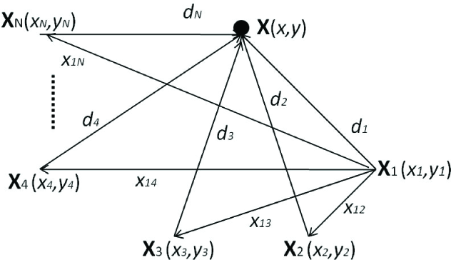
TDOA target localization scheme

Now, let us consider the triangle formed by points x, x₁ and x₂ on Figure 1. Thus, from the law of cosines it yields

d_{2}^{2} = d_{1}^{2} + {‖ x_{12} ‖}^{2} - 2 x_{12}^{T} D_{1}

(8)

where D₁ = x - x₁. From equation (5), it is follows that

f_{TDOA, 1}^{2} = d_{1}^{2} - f_{TDOA, 1}^{2} d_{1} - d_{1}^{T}

(9)

and combining equations (7) and (8), we finally obtain

x_{12}^{T} (x - x_{1}) + f_{TDOA, 1} ‖ x - x_{1} ‖ = \frac{1}{2} ({‖ x_{12} ‖}^{2} - f_{TDOA, 1}^{2})

Similar equations can be derived for triangles {x, x₁,x_j}, j = 2,3,…,N. Hence, the following nonlinear system equations are obtained

\underset{A}{\underset{⏟}{(\begin{array}{l} x_{12}^{T} & f_{TDOA, 1} \\ x_{13}^{T} & f_{TDOA, 2} \\ ⋮ & ⋮ \\ x_{1 N}^{T} & f_{TDOA, N} \end{array})}} \underset{X}{\underset{⏟}{(\begin{matrix} x - x_{1} \\ ‖ x - x_{1} ‖ \end{matrix})}} = \underset{b}{\underset{⏟}{\frac{1}{2} (\begin{matrix} {‖ x_{12} ‖}^{2} - f_{TDOA, 1}^{2} \\ {‖ x_{13} ‖}^{2} - f_{TDOA, 2}^{2} \\ ⋮ \\ {‖ x_{1 N} ‖}^{2} - f_{TDOA, N}^{2} \end{matrix})}} + \underset{e}{\underset{⏟}{(\begin{matrix} e_{1} \\ e_{2} \\ ⋮ \\ e_{N} \end{matrix})}}

(9)

where A ∈ ℝ^(N−1)×3 and X ∈ ℝ^(3×1). In the presence of noisy measurements, the above equation is affected and the measurements error vector e ∈ ℝ^(N−1)×1 must be included.

Note that if the number of base stations increases, equation (9) is over-determined. Several different approaches have been proposed for such an over determined system. In [17] and [18], improvements to the LS approach were made based on the Lagrangian multipliers optimization technique. In [17], a Linear-Corrector (LCLS) factor is added to a standard LS solution, whilst in [18], a Quadratic-Correction (QCLS) version is developed for TOA, TDOA, AOA and RSS measurements. The LCLS was applied in real-time to localize a static sound source.

Another study of static target was presented in [16] with a Constrained Weighted Least Squares (CWLS) using TDOA measurements.

In the linear-Gaussian case, the KF has a low computational complexity because only the first two moments of the probability distribution need to be stored [21, 29]. In addition, when nonlinear relationships are presented, the EKF can be employed. In real-time applications, like unmanned aerial, ground and underwater vehicles, computation time is an important factor in achieving the tasks. In this sense, the KF is attractive since it makes estimation recursively and is easy to implement.

The precision of the estimated position strongly depends on the noise in the radio signals and NLOS conditions. Furthermore, the UAV is an unstable system with very fast dynamics. The assumption of having a static target cannot be considered at all as in [3] and [24]. Then, the localization should be precise enough to at least localize the UAV in an acceptable neighbourhood of the real position.

3. UAV localization

The KF is a well-known method for localization and tracking systems, but the possible drift of the estimated state is considered to be a crucial weaknesses. This drift is indeed a serious problem, especially when the nonlinear system model is based on TDOA measurements.

3.1 Kalman filter

The KF is an algorithm for efficient state estimation minimizing the covariance error [21]. The basic filter is well-established and it is assumed that the transition and the observation models are linear. When the input is zero, such a model is given by

\begin{matrix} ϑ_{k | k - 1} = & Φ_{k | k - 1} ϑ_{k - 1 | k - 1} + w_{k | k - 1} \\ ξ_{k} = & H_{k} ϑ_{k | k - 1} + v_{k | k - 1} \end{matrix}

where ϑ_k is the state vector at time k, Φ_k is the state transfer matrix and ξ_k is the observation process. The vectors w_k and v_k are respectively noise process and measurement vectors which are assumed to be independent with Gaussian distribution, that is, w_k∼N(0,Q_k)and v_k∼N(0,Q_k).

If the process system to be estimated or the measurements system is nonlinear, the EKF should be applied. For this case, a Taylor series is used to linearize the nonlinear stochastic difference equations system around a known vector ϑ. The EKF is then applied to the linearized nonlinear process as follows

\begin{matrix} {\tilde{ϑ}}_{k + 1} \approx & {\tilde{ϑ}}_{k + 1} + A_{k} ({\tilde{ϑ}}_{k} - {\hat{ϑ}}_{k}) + W_{k} w_{k} \\ {\tilde{ξ}}_{k} \approx & ξ_{k} + B_{k} ({\tilde{ϑ}}_{k} - {\hat{ϑ}}_{k}) + V_{k} v_{k} \end{matrix}

where ${\hat{ϑ}}_{k}$ is the current estimate state vector and A_k, B_k, W_k and V_k are the Jacobian matrices

\begin{matrix} A_{k} = {\frac{\partial f (ϑ_{k}, k)}{\partial ϑ} |}_{ϑ = {\hat{ϑ}}_{k}}, & B_{k} = {\frac{\partial h (ϑ_{k}, k)}{\partial ϑ} |}_{ϑ = {\hat{ϑ}}_{k}} \\ W_{k} = {\frac{\partial f (ϑ_{k}, k)}{\partial w} |}_{ϑ = {\hat{ϑ}}_{k}}, & V_{k} = {\frac{\partial h (ϑ_{k}, k)}{\partial v} |}_{ϑ = {\hat{ϑ}}_{k}} \end{matrix}

where f(ϑ_k,k) and h(ϑ_k,k) are the nonlinear process and observation functions, respectively. The reader can find more details on the KF in [29] and [30].

3.2 Localization

In this part, we develop the localization algorithm for a UAV. To simplify, we will consider the following assumptions:

The workspace of the flying robot is the XY plane defined by four base stations.

The translational movements are given in manual mode.

An onboard attitude control stabilizes the orientation of the UAV.

Linear motion at constant velocity is performed by the vehicle.

Under these assumptions, the localization problem reduces to estimate the position and velocity of the aircraft in a plane. Consequently, the state transfer matrix, A_k, yields a 4 × 4 constant matrix

A_{k} = (\begin{matrix} 1 & 0 & Δ & 0 \\ 0 & 1 & 0 & Δ \\ 0 & 0 & 1 & 0 \\ 0 & 0 & 0 & 1 \end{matrix})

where A is the constant sampling period of the TDOA measurements. We are using a sampling period of 100 milliseconds. Therefore, the state vector,^, only contains the UAV position and velocity components, i.e.,

\begin{matrix} ϑ_{k} = & {(\begin{matrix} ϑ_{k}^{p} & {\dot{ϑ}}_{k}^{p} \end{matrix})}^{T} \\ = & {(\begin{matrix} x_{k} & y_{k} & {\dot{x}}_{k} & {\dot{y}}_{k} \end{matrix})}^{T} \end{matrix}

From equation (1), note that the observed process is not linear and the function ξ_k = h(ϑ_k, k) becomes

ξ_{k} = (\begin{matrix} \sqrt{{(x_{k} - x_{1})}^{2} + {(y_{k} - y_{1})}^{2}} \\ \sqrt{{(x_{k} - x_{2})}^{2} + {(y_{k} - y_{2})}^{2}} \\ \sqrt{{(x_{k} - x_{3})}^{2} + {(y_{k} - y_{3})}^{2}} \\ \sqrt{{(x_{k} - x_{4})}^{2} + {(y_{k} - y_{4})}^{2}} \end{matrix}) = (\begin{matrix} ‖ ϑ_{k}^{p} - x_{1} ‖ \\ ‖ ϑ_{k}^{p} - x_{2} ‖ \\ ‖ ϑ_{k}^{p} - x_{3} ‖ \\ ‖ ϑ_{k}^{p} - x_{4} ‖ \end{matrix})

(10)

The Jacobian matrix B_k for equation (10) is

B_{k} = (\begin{matrix} \frac{x_{k} - x_{1}}{‖ ϑ_{k}^{p} - x_{1} ‖} & \frac{y_{k} - y_{1}}{‖ ϑ_{k}^{p} - x_{1} ‖} & 0 & 0 \\ \frac{x_{k} - x_{2}}{‖ ϑ_{k}^{p} - x_{2} ‖} & \frac{y_{k} - y_{2}}{‖ ϑ_{k}^{p} - x_{2} ‖} & 0 & 0 \\ \frac{x_{k} - x_{3}}{‖ ϑ_{k}^{p} - x_{3} ‖} & \frac{y_{k} - y_{3}}{‖ ϑ_{k}^{p} - x_{3} ‖} & 0 & 0 \\ \frac{x_{k} - x_{4}}{‖ ϑ_{k}^{p} - x_{4} ‖} & \frac{y_{k} - y_{4}}{‖ ϑ_{k}^{p} - x_{4} ‖} & 0 & 0 \end{matrix})

(11)

Notice that all elements of equation (11) have singularities if ‖ϑ^p_k−x_i| = 0, i =1,2,3,4.

4. Experimental Set-up

4.1 Quadrotor Vehicle

The flying robot is a classical quadrotor which is mechanically simpler than a classical helicopter since it does not have a swashplate and it have constant pitch blades, see Figure 2. It has two counter rotating pairs of propellers arranged in a square. The onboard computer, the IMU, the location sensor board and the batteries are mounted in the middle of the square.

Figure 2.

Quadrotor UAV

The thrust is provided by four Robbe Roxxy BL-Motor 2827-34 brushless motors and four YGE30i speed controllers. A homemade IMU is used to compute the attitude angles. The roll φ, pitch θ and yaw Ψ angles are estimated by using a three-axis accelerometer (ADXL203) and a compass module (CMPS03). The angular rates, $\dot{φ}$ and $\dot{θ}$ , are measured by an integrated dual axis gyroscope (IDG-500), and the yaw angle rate, $\dot{ψ}$ , is measured by a single yaw rate gyroscope (ADXRS613). The altitude is determined using an ultrasonic sensor (SPF03).

The onboard hardware is based on a RCM3400 analogue RabbitCore which runs at 29.4 MHz. An I2c protocol control signal is sent to the speed controllers every sampling period. The attitude dynamic is stabilized onboard using the nested saturation control [31].

4.2 Distance Measurement System

The NanoLOC development kit from Nanotron Technologies has been used to measure the distances between the BS. Nanotron Technologies has developed a WSN which can work as a Real-Time Location Systems (RTLS) [10]. The distance between two wireless nodes is determined by their Symmetrical Double-Sided Two Way Ranging (SDS-TWR) technique, which allows a distance measurement by means of the signal propagation delay. It estimates the distance between two nodes by measuring the TDOA symmetrically from both sides.

Wireless communications as well as the ranging methodology SDS-TWR are integrated in a single chip, the NanoLOC TRX Transceiver [32]. The transceiver operates in the ISM band of 2.4 GHz and supports location-aware applications including Location Based Services (LBS) and asset tracking applications. The wireless communication is based on Nanotron's patented modulation technique CSS according to the wireless draft standard IEEE 802.15.4a.

SDS-TWR measures the round trip time and avoids the need to synchronize the clocks. Time measurement starts in Node A by sending a package. Node B starts its measurement when it receives this packet from Node A and stops when it sends it back to the former transmitter. When Node A receives the acknowledgment from Node B, the accumulated time values in the received packet are used to calculate the distance between the two stations. The difference between the time measured by Node A and the time measured by Node B is twice the time of signal propagation. To avoid the drawback of clock drift, the range measurement is preformed twice and symmetrically. A ranging measurement, DAB, between Node A and Node B is obtained using the following formula [28]

D_{A B} = \frac{(T_{1} - T_{2}) + (T_{3} - T_{4})}{4}

where T₁ is the propagation delay time of a round trip between Node A and Node B, T₂ is the processing delay in Node B, T₃ is the propagation delay time of a round trip between Node B and Node A, and T₄ is the processing delay in Node A. Time instants T_i are approximately four milliseconds and an accuracy smaller than one metre can be obtained [28]. Furthermore, environmental conditions can affect the accuracy of the measured distances.

The NanoLOC development kit contains five sensor boards with sleeve dipole omnidirectional antennas. One target board, TAG board, is mounted in the UAV and the base station boards are placed in the desired geometry. In our case, we chose a rectangular geometry (see Figures 4 and 10).

Figure 3.

Kalman filter implementation set-up

Figure 4.

Estimation position in hover flight

To measure the real distances between the helicopter and the base stations, a wireless link is added. This link is made by using two XBee-PRO modems that connect the helicopter to an external computer where the algorithm is executed in real-time. Figure 3 shows the real-time closed-loop localization algorithm scheme. The target board and the BS boards exchange data. Then, the TAG board sends a codified message with the measured distances via the serial communication link to a XBee-PRO modem. This last message is sent immediately to another XBee-PRO connected to a computer where the algorithm is executed in real-time. A frame data of 68 bytes is decoded to find out the four actual measured distances values d¹_k, d²_k, d³_k and d⁴_k. Finally, the innovation v_k = y_k−ŷk, is computed

v_{k} = (\begin{matrix} d_{k}^{1} - ‖ {\hat{ϑ}}_{k}^{p} - x_{1} ‖ \\ d_{k}^{2} - ‖ {\hat{ϑ}}_{k}^{p} - x_{2} ‖ \\ d_{k}^{3} - ‖ {\hat{ϑ}}_{k}^{p} - x_{3} ‖ \\ d_{k}^{4} - ‖ {\hat{ϑ}}_{k}^{p} - x_{4} ‖ \end{matrix})

(12)

The prediction and the update steps of the localization algorithm are performed at = 100ms. Once these tasks have completed ${\hat{ϑ}}_{k | k - 1}$ , ${\hat{ϑ}}_{k + 1 | k + 1}$ , $P_{k | k - 1}$ , $P_{k + 1 | k + 1}$ ), a one step Kalman smoother is executed to obtain ϑ_k+1|k+1 and P_k+1|k+1, see Figure 3.

Even if the KF (and also other approaches) is common, the convergence is not totally ensured if initial conditions are badly conditioned. Moreover, if we want to carry out trajectory tracking tasks, it is necessary to improve the above algorithms. Notice that the UAV is an unstable system with very fast dynamics where no convergence of one state could be critical.

5. Experimental Results

Experiments have been carried out indoors with the UAV flying in manual mode. Sets of data were collected several times (over 40 seconds) to verify the correct functioning of the proposed localization algorithm in closed-loop. The covariance values of matrices R and Q were adjusted to obtain an acceptable filter response. The final values are R = 0.45I and Q = 10 × 10⁻⁵I. The Jacobian matrices W_k and V_k are considered as identity matrices.

5.1 Hover Flight Test

The workspace of the UAV is delimited by the BS placed in positions BS1 =(0,0), BS₂ =(0,4.5m), BS₃ =(4.5m,4m) and BS₄=(0,4m), see Figure 4. The experiment consists of a hover flight of the UAV over the point (1.75m, 2m). Figure 4 show the estimated position when the algorithm is applied in real-time. Note that the UAV estimated position remains around the desired point during all experiments. Figure 5 illustrates the histograms for ◯ and ŷ which are approximately Gaussian with mean values μ_◯=1.5713m and μ_ŷ=2.1685m, and standard deviations σ_◯=0.1374m and σ_ŷ=0.1224m.

Figure 5.

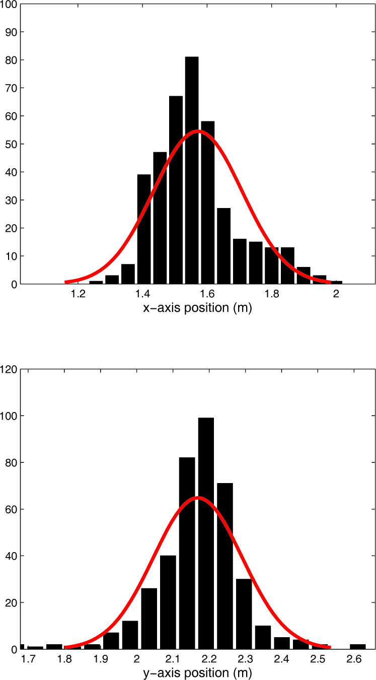
Histograms for ◯ and ŷ

Another way to evaluate the performance of the proposed algorithm is through confidence intervals as shown in Figure 6. From this graph, we can see that the estimated position remains within the confidence interval, i.e., 90% of data are around the mean value and very few values are beyond this range. Therefore, we conclude that the proposed location algorithm correctly estimates the position of the UAV in hover, with a relatively small error.

Figure 6.

Variances of x and y in hover flight

Remember that the helicopter is hovering and from Figure 7 note that the estimated speeds are close to zero in hover flight, speed must be zero or at least very close to zero The pick values (∼ 1 m/s) follow from the small corrections given by the pilot.

Figure 7.

Estimated velocities in hover flight

5.2 Path Following Flight Test

In this part, the experiment is devoted to evaluating the path following accuracy of the proposed localization algorithm. In order to allow sufficient movement for the UAV, a larger workspace is used. In this case, the base stations were place at points BS₁ =(0,0), BS₂ =(0,8.5m), BS₃ =(8.5m,6m) and BS₄ =(0,6m).

Three parts are included in this experiment, see Figure 8. The first and third parts are devoted to trajectory tracking, whereas the second one is dedicated to hover flight. Thus, from t₀ to t₁ the pilot moves the UAV following a straight line from point (1.75m, 2m) to point (6m, 5m). From Figures 9 and 11a, note that both ◯ and ŷ are a little far from the desired path. This is because when the UAV was launched, the pilot tried to bring the UAV along the path. This fact can also be observed in the estimated speeds shown in Figure 10. The velocity magnitudes are great at the beginning which expresses the abrupt linear movements of the vehicle given by the pilot.

Figure 8.

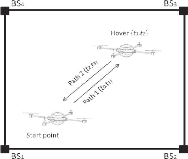
Experimental path following set-up

Figure 9.

Estimated ◯ and ŷ in path following

From t₁ to t₂, Figure 11b, the helicopter is in hover flight over the point (6m, 5m). We note that during this period, the best estimation is obtained, see also Figure 9. Finally, from t₂ to t₃ the helicopter returns to the starting point (Figure 11c). From Figures 9 –11 we can conclude that for tracking, and obviously for hover, the results are satisfactory.

It is also important to point out that commonly in path following applications, the state transfer matrix Ak is derived from the accelerated motion and this kind of dynamic is not considered here. However, we note that, in our study, the estimated position is good with a relatively small error.

Figure 10.

Estimated velocities in path following

Figure 11.

Estimated position in path following. Path 1 (top), hover (middle), path 2 (bottom)

6. Conclusions

Real-time estimation of position and velocity of a UAV has been presented in this paper by using the time difference of arrival method applied to a Local Positioning System (LPS). This application is original because it offers an alternative method for localizing UAVs indoors. The LPS is composed of five transceiver cards which exchange information between them.

The obtained TDOA measurements model is nonlinear and an EKF was applied in order to estimate the states. The proposed localization algorithm has been successfully tested in closed-loop real-time experiments for hover flight and for path flight tracking. The best results were found in the hover test and this performance is related to the form of the transfer matrix.

To improve the path tracking task, the accelerated motion must be included in A_k. However, with quasi-constant displacement, the algorithm continues making a good estimation of position. Finally, the experimental results have proved the good performance of the proposed algorithm with small errors.

Current research is focused on including the proposed localization algorithm into the stabilization control loop of the UAV. We are working to carry out autonomous navigation experiments with a UAV.

Footnotes

7. Acknowledgements

The first author thanks the Universidad Autónoma del Carmen (UNACAR) and the Secretaría de Educación Pública (SEP), both from Mexico, for their financial support PROMEP/103.5/07/2057.

References

Yim

Park

Joo

Jeong

(2008) Extended Kalman Filter to wireless LAN based indoor positioning. Decision and Support Systems (Elsevier) 45, 960–971.

Yim

Jeong

Gwon

Joo

(2010) Improvement of Kalman filters for WLAN based indoor tracking. Expert Systems Applications (Elsevier) 37(1), 426–433

Röhrig

Spieker

(2008) Tracking of transport vehicles for warehouse management using a wireless sensor network. In: 2008 IEEE/RSJ International Conference on Intelligent Robots and Systems, Nice, France, September 22–26.

Röhrig

Muller

(2009) Localization of sensor nodes in a wireless sensor network using the nanoLOC TRX transceiver. In: IEEE 69th Vehicular Technology Conference Spring, Barcelona, Spain, April 26–29.

Soriano

Caballero

Ollero

(2009) RF-based particle filter localization for wildlife tracking by using an UAV. On: 40th International Symposium of Robotics, Barcelona, Spain.

Togersen

F.A.

Skjoth

Munksgaard

Hojsgaard

(2010) Wireless indoor tracking network based on Kalman filters with an applications to monitoring dairy cows. Computer and Electronics in Agriculture (Elsevier) 72, 119–126

Wendel

Meister

Schlaile

Trommer

G.F.

(2006) An integrated GPS/MEMS-IMU navigation system for an autonomous helicopter. Aerospace Science Technology 10, 527–533.

Kim

Sukkarieh

Wishart

(2003) Real-time navigation, guidance and control of an UAV using low-cost sensors. In: International Conference of Field and Service Robotics (FSR'03), Yamanashi, Japan, pp. 95–100.

Bristeau

P.-J.

Dorveaux

Vissière

Petit

(2010) Hardware and software architecture for state estimation on an experimental low-cost small-scaled helicopter. Control Engineering Practice 18, 733–746.

10.

Nanotron Technologies GmbH (2006) Real Time Localization Systems (RTLS). White paper.

11.

De Nardis

Di Benedetto

M.-G.

(2007) Overview of the IEEE 802.15.4/4a standards for low data rate wireless personal data networks. In: 4th Workshop on Positioning, Navigation and Communication, Hannover, Germany.

12.

Ahn

H.-S.

Hur

Choi

W.-S.

(2008) One-way ranging technique for CSS-based indoor localization. In: IEEE International Conference on Industrial Informatics, Daejeon, Korea.

13.

Torrieri

D.J.

(1984) Statistical theory of passive location systems. IEEE Transactions on Aerospace Electronic Systems. AES-20(2), 183–198.

14.

Mao

Fidan

Anderson

B.D.O.

(2007) Wireless sensor network localization techniques. Computers Networks 51(10), 2529–2553.

15.

Seco

Jiménez

Prieto

Roa

Koutsou

(2009) A survey of mathematical methods for indoor localization. In: IEEE 6th International Symposium on Intelligent Signal Processing, Budapest, Hungry, August 26–28.

16.

Dogancaya

Hashemi-Sakhtsari

(2005) Target tracking by time difference of arrival using recursive smoothing. Signal Process. 85, 667–679.

17.

Huang

Benesty

Elko

G.W.

Mersereati

R.M.

(2001) Real-time passive source localization: A practical linear correction least-squares approach. IEEE Transactions on Speech and Audio Processing 9(8), 943–956.

18.

Cheung

K.W.

H.C.

W.-K.

Chan

Y.T.

(2006) A constrained least squares approach to mobile positioning: Algorithms and optimality. EURASIP Journal of Applied Signal Processing 1–23. Article ID 20858.

19.

Smith

J.O.

Abel

J.S.

(1987) Closed-form least-squares location estimation from range-difference measurements. IEEE Transactions on Acoustic and Speech Signal Processing ASSP-35, 1661–1669.

20.

Chan

Y.T.

K.C.

(1994) A simple and efficient estimator for hyperbolic location. IEEE Transactions on Signal Process. 42(8), 1905–1915.

21.

Kalman

R.E.

(1960) A new approach to linear filtering prediction problems. ASME Journal of Basic Engineering 82, 34–45

22.

Becerra

V.M.

Roberts

P.D.

Griffiths

G.W.

(2001) Applying the extended Kalman filter to systems described by nonlinear differential-algebraic equations. Control Engineering Practice 9(3), 267–281.

23.

Julier

S.J.

Ulhmann

J.K.

(1995) A new extension of the Kalman filter to nonlinear systems. In: Proceedings of the American Control Conference, pp. 1628–1630.

24.

Cho

Lee

C.W.

Ban

S.J.

Kim

S.W.

(2010) An enhanced positioning scheme for chirp spread spectrum ranging. Expert Systems with Applications 37(8), 5728–5735.

25.

Röhrig

Spieker

(2008) Localization of pallets in warehouses using wireless sensor networks. In: 16th Mediterranean Conference on Control and Automation, pp. 1833–1838.

26.

Bechler

Grimm

Kroschel

(2003) Speaker tracking with a microphone array using Kalman filtering. Advances in Radio Science 1, 113–117.

27.

Liang

Dai

(2008) Robust tracking of moving sound source using multiple model Kalman filter. Applied Acoustics 69, 1350–1355.

28.

Nanotron Technologies GmbH (2008) nanoLOC Development Kit User Guide. Technical Report NA-06-0230-0402-2.0.

29.

Bar-Shalom

X.-R.

Kirubarajan

(2001) Estimation with Applications to Tracking and Navigation. Wiley, New York.

30.

Grewal

M.S.

Andrews

A.P.

(2001) Kalman Filtering: Theory and Practice using MATLAB. Wiley-Interscience Publication, New York.

31.

Sanahuja

Castillo

Sanchez

(2010) Stabilization of n integrators in cascade with bounded input with experimental application to a VTOL laboratory system. International Journal of Robust Nonlinear Control 20(10), 1129–1139. doi:10.1002/rnc.1494

32.

Nanotron Technologies GmbH (2008) nanoLOC TRX Transceiver (NA5TR1) User Guide. Datasheet NA-06-0230-0385-2.00.

Indoor Localization of a Quadrotor Based on WSN: A Real-Time Application

Abstract

Keywords

1. Introduction

2. Measurements Models

2.1 Localization algorithm based on TDOA measurements

3. UAV localization

3.1 Kalman filter

3.2 Localization

4. Experimental Set-up

4.1 Quadrotor Vehicle

4.2 Distance Measurement System

5. Experimental Results

5.1 Hover Flight Test

5.2 Path Following Flight Test

6. Conclusions

Footnotes

7. Acknowledgements

References