Sage Journals: Discover world-class research

Abstract

A redundant robot has more degrees of freedom (DOF) than those required to accomplish a given motion task. This fact allows the possibility of achieving an additional task, such as avoidance of joint limits or singularities, besides the primary one. Different criteria have been proposed in the literature for the selection of such a secondary task. This paper first recalls some of those criteria and then proposes a two-loop scheme for the motion control of redundant robots. In order to validate the proposed scheme, some experiments are carried out in a direct-drive redundant planar arm which has been designed and built in our laboratory.

Keywords

Redundant Manipulators Two-Loop Control Modelling Experimental Evaluation

1. Introduction

Redundant manipulators have been a theme of study for researchers and engineers in the last years. Kinematic redundancy appears in robot manipulators which have more degrees of freedom than those necessary for achieving a given task. This can be considered a source of more dexterity for the robot since, due to the extra degrees of freedom, some additional tasks, such as the avoidance of obstacles or singularities, can be performed while executing the primary motion task [1, 2].

A very common task in robotics is to control the pose (that is, the position and orientation) of the robot end–effector. And it is a well–known fact that the pose is specified by means of six independent variables for motion in 3D space, while only three are required if the motion is constrained to the plane (2D). According to this, a redundant robot for pose control should have either more than six degrees of freedom for spatial motion or more than three for planar motion. However, there are some cases in which the desired task is not to control the whole pose of the end–effector; in such cases we talk about functional redundancy [3]. For example, a 3-dof robot manipulator is functionally redundant if the desired task involves controlling only the position (two coordinates) of the robot end–effector, but it is not if both position and orientation are specified as part of the task.

In an n-dof serial robot manipulator the configuration of the end–effector is determined by means of n joint coordinates. On the other hand, the desired motion task to be performed by the robot is specified by m operational coordinates, where it is assumed that m≤n so that the task can be achieved. Notice that in this paper we use the term operational coordinates, instead of pose coordinates, in order to include cases such as the aforementioned planar robot, in which we have three joint coordinates and only two operational coordinates.

The function which allows to obtain the operational coordinates q̇ ∈ ℝ^m from the joint coordinates q̇ ∈ ℝⁿ is known as direct kinematics. In a serial robot (either redundant or not) a unique solution to the problem of direct kinematics always exists; however, that is not true for the inverse kinematics problem (to obtain the joint coordinates from the operational coordinates). In the case of a non-redundant robot the inverse kinematics can have either no solution, only one solution, or multiple isolated solutions; if the robot is redundant then an infinite number of solutions can be found for the same operational configuration of the end–effector. The fundamental problem of redundant robots is to find the best solution to inverse kinematics that allows not only the fulfillment of the primary motion task, but also the accomplishment of a secondary task.

Several schemes for inverse kinematics of redundant manipulators have been proposed in the literature, as indicated in recent works such as [4] or [5]; among these, the so–called closed–loop inverse kinematics, or CLIK algorithm, proposed by [6], is one of the most commonly employed.

In this paper we propose the use of a two–loop scheme for the control of redundant robots which is based on the CLIK algorithm. It is important to mention that similar controllers have already been proposed (see, e.g., [7]) but using a different inner loop. The proposed controller is completed using the well–known gradient projection method for dealing with the secondary task.

The aim of this paper is then twofold. First after recalling the main aspects related with redundancy resolution, we propose the two–loop controller and show how it ensures the convergence to the primary and secondary tasks. Secondly, in order to validate the performance of the proposed controller on a real robot, we show the results of some experiments carried out in a planar functionally redundant arm which is in our laboratory.

The remainder of the paper is organized as follows. A review of the basic methods of redundancy resolution can be found in Section 2. The two–loop control scheme, including its stability analysis, is proposed in Section 3. The characteristics and mathematical model of the planar arm employed in the experiments are described in Section 4, while the results of testing different secondary tasks are shown in Section 5. Finally, Section 6 is devoted to the conclusions of the work.

2. Redundancy Resolution

There exist two main approaches for obtaining the inverse kinematics in redundant manipulators [8]: local optimization and global optimization. This paper only considers the local optimization approach [9], which is explained in this section.

Let us start from the robot direct kinematics function, given by

x = f (q)

(1)

where q̇ ∈ ℝ^m is the vector of joint coordinates and xeR^mis the vector of operational coordinates. Taking the time derivative of (1) we get:

\dot{x} = J (q) \dot{q}

(2)

where q̇ ∈ ℝⁿ is the analytical Jacobian of the robot. Figure 1 shows the mapping between the space of joint velocities q̇ ∈ ℝⁿ and the space of operational velocities q̇ ∈ ℝ^m, given by matrix J in (2).

Figure 1.

Mapping between joint and operational velocity spaces.

Figure 1 also shows two subspaces of great interest [10]. One, the range space of J, ℜ(J), defined as

ℜ (J) = {J \dot{q} \in ℝ^{m} : \dot{q} \in ℝ^{n}}

is a subspace of ℝ^m that physically represents all the operational velocities which can be reached by the manipulator; the other is a subspace of ℝⁿ known as the null space of J, ℵ(J), defined as

ℵ (J) = {\dot{q} \in ℝ^{n} : J \dot{q} = 0}

which physically represents the joint velocities that produce no operational velocity in the end–effector.

The existence of a subspace ℵ(J) ≠ Ø in a redundant manipulator allows the possibility of using methods for handling the redundant degrees of freedom and carrying out additional tasks while the primary motion task is executed.

The general method for the solution of (2) was first proposed by [11] using generalized inverses. When using the right pseudoinverse of J, denote here J^† and defined as J^†=J^T(JJ^T)¹, so that JJ⁺=I, such general solution becomes

\dot{q} = J^{†} \dot{x} + (I - J^{†} J) {\dot{q}}_{0} .

(3)

Notice that if (3) is left-multiplied by J then (2) is obtained, independently of q̇₀. This is because the term (I-J†J) acts as the orthogonal projection matrix onto the null space of J; in other words, the second term of the right–hand side of (3) always belongs to ℵ(J). In particular, if J is full rank, all the joint velocities of the form (3) exactly produce the same operational velocities in the end–effector. Moreover, q̇₀ acts as a joint velocity which can be chosen so that it makes possible to complete a secondary task, without affecting the motion of the end–effector.

Several methods have been proposed in the literature in order to select a suitable q̇₀ for a given task. In the following subsection we recall a very common strategy which is based on the optimization of a cost function.

2.1 Gradient-projection method

Introduced by [11]; this method starts from considering that vector q₀ is the gradient of a cost function H(q̇), and is weighted by the parameter α, that is to say: q̇₀=α∇H(q).

In this way, if α>0 then q̇₀ represents a joint velocity which makes H(q̇) to maximize; on the contrary, if α < 0 then q̇₀ leads to the minimization of H(q̇)

The general expression for redundancy resolution using the gradient projection method is:

\dot{q} = J^{†} \dot{x} + (I - J^{†} J) \nabla H (q)

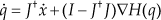
Some cost functions that are commonly employed in the literature are:

Distance from joint limits:

H (q) = {\sum_{i = 1}^{n} (\frac{q_{i} - q_{i, c}}{q_{i, \max} - q_{i, \min}})}^{2},

(4)

where (q_i,max - q_i,min) is the available range of operation for the i-th joint, and q_i,c is the central point in such a range; by minimizing, this function we keep all of the joints near of their corresponding central points, that is, far from the joint limits.

Potential energy:

H (q) = U (q),

(5)

where U(q) represents the potential energy of the manipulator; maximizing or minimizing this measure can be useful to improve the performance of the robot.

Manipulability measure:

H (q) = \sqrt{\det (J (q) J^{T} (q));}

(6)

maximizing this measure causes the robot to move away, as far as possible, from singular configurations.

The three cost functions previously mentioned are the ones employed during the experiments described in Section 5.

3. Two–Loop Control of Redundant Robots

The dynamics of a serial n-joint robot manipulator without friction can be described as [12]:

M (q) \dot{q} + C (q, \dot{q}) \dot{q} + g (q) = τ

(7)

where M(q)∈ℝ^n×n is the symmetric and positive definite manipulator inertia matrix, C(q,q̇) ∈ ℝ^n×n is the matrix of centrifugal and Coriolis torques, g(q) ∈ ℝⁿ is the vector of gravitational torques, which turns out to be the gradient of the potential energy of the robot (i.e., g(q) = ∇U(q)), and τ is the vector of external torques applied to the robot.

There exist several schemes for the control of redundant robots, although most of them employ a two–step procedure: first, using an inverse kinematics algorithm such as (3), the desired joint velocities q̇_d are computed from both the desired operational velocities ẋ_d, required for the motion task, and q̇₀, which is chosen according to the desired redundant task; secondly, a joint-space controller using as input q̇_d (or both q̇_d and its time integral q_d), produces the required torques for each of the robot joint actuators. Figure 2 shows a general diagram of this two–stage controller.

Figure 2.

Classical controller with redundancy resolution.

Given x_d and q₀, the simplest algorithm for inverse kinematics with redundancy resolution would be to use

{\dot{q}}_{d} = J^{†} (q_{d}) {\dot{x}}_{d} + [I - J^{†} (q_{d}) J (q_{d})] {\dot{q}}_{0}

(8)

to compute q_d, and then to employ numerical integration to get q_d for the next iteration. The use of (8) is avoided, however, due to the fact that, as the algorithm does not depend on x_d but on x_d, the convergence to x_d can not be ensured; moreover, due to the numerical integration, a small though unavoidable error appears, which leads to a long-term deviation of the estimated q_d from the exact one.

Algorithmic solutions that overcome these problems are based on the use of a feedback correction term; these are termed closed–loop inverse kinematics (CLIK) algorithms [4]. A very common CLIK algorithm is

{\dot{q}}_{d} = J^{†} (q_{d}) {{\dot{x}}_{d} + K [x_{d} - f (q_{d})]} + [I - J^{†} (q_{d}) J (q_{d})] {\dot{q}}_{0}

(9)

where K is a positive definite diagonal matrix of constant gains, and f(·) is the robot direct kinematics function.

As mentioned in [13], the structure of the CLIK algorithm can be conceptually adopted for a simple robot control technique, known under the name of kinematic control, which assumes that the control inputs to the robot joints are velocity commands, instead of torque commands. The rationale behind this assumption is the fact that most of robot actuators (usually brushless DC motors) are driven by electromechanical drives which can be configured in velocity mode, that is, with inner velocity controllers. For more information on brushless DC motors and their operation modes see [14].

Following the idea in [15], in this paper we propose the use of a two–loop control scheme for redundant manipulators. In such scheme an outer kinematic controller is devoted to generate the joint velocity commands for the inner velocity controller. Figure 3 shows a general diagram of this scheme.

Figure 3.

Two–loop control scheme.

In this paper we consider as outer loop the following kinematic controller, based on the CLIK methodology:

ν_{d} = J^{†} (q) [{\dot{x}}_{d} + K \tilde{x}] + [I - J^{†} (q) J (q)] {\dot{q}}_{0},

(10)

where x˜ = x_d-x and K is a positive definite matrix of control gains. Notice that (10) has the same structure of (9) but now we feedback the actual joint coordinates q to compute the desired joint velocities, now named v_d instead of q_d for the sake of clarity.

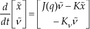
In the inner loop we propose the use of the following velocity controller, which requires the knowledge of the robot dynamic model [15]:

τ = M (q) [{\dot{ν}}_{d} + K_{v} \tilde{ν}] + C (q, \dot{q}) \dot{q} + g (q),

(11)

where v˜ = v_d-q̇, v̇_d is the time derivative of (10), computed numerically, and K_v is a diagonal matrix of positive gains.

3.1 Stability Analysis

This section describes the stability analysis of the two-loop controller (10)–(11) when applied to the robot dynamics (7). For the analysis, let us consider that, during the execution of the assigned task, the robot never passes through singular points (where J(q) losses its full rank);

moreover, it is assumed that J(q) is always bounded by a positive constant k_J, that is to say:

∥ J (q) ∥ \leq k_{J}, \forall q \in ℝ^{n} .

The first step is to left–multiply (10) by J, to obtain

J ν_{d} = {\dot{x}}_{d} + K \tilde{x},

and as v˜ = v_d-q̇, then $J \tilde{v} = J ν_{d} - J \dot{q} = \dot{\tilde{x}} + K \tilde{x}$ , where (2) has been used. On the other hand, replacing the controller (11) in the robot dynamics (7) yields to

\dot{\tilde{ν}} + K_{ν} \tilde{ν} = 0

where $\dot{\tilde{ν}} = \frac{d}{d t} \tilde{ν} = {\dot{ν}}_{d} - \dot{q}$

The closed-loop system is thus written simply as

\frac{d}{d t} [\begin{matrix} \tilde{x} \\ \tilde{ν} \end{matrix}] = [\begin{matrix} J (q) \tilde{ν} - K \tilde{x} \\ - K_{ν} \tilde{ν} \end{matrix}]

(12)

and it is observed that it is a non-autonomous system with a unique equilibrium in the origin of the state space [x˜^Tv˜^T] ^T ∈ℝ ^n+m . In order to verify the stability of this equilibrium we use the following Lyapunov function:

V (\tilde{x}, \tilde{ν}) = \frac{1}{2} γ {\tilde{x}}^{T} x + \frac{1}{2} {\tilde{ν}}^{T} \tilde{ν},

with γ such that

0 < γ < \frac{4}{k_{J}^{2}} λ_{m} {K_{ν}} .

(13)

where λ_m{·} stands for the smallest eigenvalue of the corresponding matrix.

It is clear that V(x˜,v˜)is positive definite, and is easy to verify that its time derivative

\dot{V} (\tilde{x}, \tilde{ν}) = - γ {\tilde{x}}^{T} K \tilde{x} - {\tilde{ν}}^{T} K_{ν} \tilde{ν} + γ {\tilde{x}}^{T} J (q) \tilde{ν}

is negative definite whenever (13) is satisfied.

This analysis allows us to conclude that the equilibrium of (12) is locally asymptotically stable, meaning that the motion control aim is fulfilled, i.e. limx(t) lim x→+x_d (t), at least for a region close enough to x_d(t) which includes no singular points of the jacobian J (q). On the other hand, the use of a gradient method for redundancy resolution assures the optimization of the cost function used as a secondary task [11].

4. 3-DOF Planar Robot

This section is devoted to the description and mathematical modeling of the 3–dof robot arm that has been designed and built in our laboratory, and was used during the experiments presented in Section 5. Both a photograph of such mechanism and a diagram showing its characteristic parameters are displayed in Figure 4.

Figure 4.

3–DOF planar robot used in experiments.

The robot consists of three direct–drive actuators, models DM1200A, DM1030B and DM1004C from Parker Compumotor, which are brushless DC motors; the drives of such motors can be configured to operate in either position, velocity or torque mode, depending on what signal is used as the command input for the drive. The robot links are made out of aluminum, due to its light weight and rigidity.

4.1 Kinematic Model

The direct kinematic model of the 3–dof arm, considering it as a non–redundant robot, is given by:

[\begin{array}{l} x \\ y \\ ϕ \end{array}] = [\begin{array}{l} l_{1} s_{1} + l_{2} s_{12} + l_{3} s_{123} \\ - l_{1} c_{1} - l_{2} c_{12} - l_{3} c_{123} \\ q_{1} + q_{2} + q_{3} - \frac{π}{2} \end{array}]

(14)

where [x y]^T ∈ ℝ² represents the position, and φ ∈ ℝ the orientation of the end–effector in the plane; li is the length of the i-th link; the simplified notation for sine and cosine functions (s_i = sin(q_i), c_ij = cos(q_i + q_j), etc.) is used.

The inverse model of (14) is obtained in [13], and it is:

[\begin{matrix} atan 2 (G_{1}, F_{1}) \\ atan 2 (G_{2}, F_{2}) \\ ϕ - q_{1} - q_{2} + \frac{π}{2} \end{matrix}]

(15)

where

\begin{array}{l} G_{1} = \frac{(l_{1} + l_{2} F_{2}) p_{w x} + l_{2} G_{2} p_{w y}}{p_{w x}^{2} + p_{w y}^{2}}, \\ G_{2} = \pm \sqrt{1 - F_{2}^{2}}, \\ F_{1} = \frac{- (l_{1} + l_{2} F_{2}) p_{w y} + l_{2} G_{2} p_{w x}}{p_{w x}^{2} + p_{w y}^{2}}, \\ F_{2} = \frac{p_{w x}^{2} + p_{w y}^{2} - l_{1}^{2} - l_{2}^{2}}{2 l_{1} l_{2}}, \end{array}

p_wx = × − l₃ cos(φ), and p_wy = y − l₃ sin (φ).

Now, to consider the robot as redundant, only the position part of the end-effector pose is taken into account, and the last row of (14) is discarded. In such a case, the Jacobian matrix is given by

J (q) = [\begin{array}{l} l_{1} c_{1} + l_{2} c_{12} + l_{3} c_{123} l_{2} c_{12} + l_{3} c_{123} l_{3} c_{123} \\ l_{1} s_{1} + l_{2} s_{12} + l_{3} s_{123} l_{2} s_{12} + l_{3} s_{123} l_{3} s_{123} \end{array}]

and it should be noticed that this Jacobian loses rank when [q₂ q₃]^T = [mπ nπ]^T, for any integers m and n.

4.2 Dynamic model

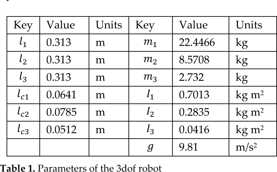
To compute the dynamic model of our robot we first employed an AutoCAD model to determine the dynamic parameters of each link i, i.e., mass (m_i), distance to the center of mass (l_ci) and moment of inertia (I_i). Then we used those parameters as inputs for the Robotica package [16], which runs under Mathematica, to obtain the components of the robot dynamics (7). The elements of the resulting matrices are:

\begin{aligned} M_{11} = & m_{1} l_{c 1}^{2} + m_{3} (l_{1}^{2} + l_{2}^{2} + l_{c 3}^{2} + 2 l_{1} l_{2} c_{2} + 2 l_{1} l_{c 3} c_{23} + 2 l_{2} l_{c 3} c_{3}) \\ ​ & + m_{2} (l_{1}^{2} + l_{c 2}^{2} + 2 l_{1} l_{2} c_{2}) + I_{1} + I_{2} + I_{3}, \\ M_{12} = & M_{21} = m_{3} (l_{2}^{2} + l_{c 3}^{2} + l_{1} l_{2} c_{2} + l_{1} l_{c 3} c_{23} + 2 l_{2} l_{c 3} c_{3}) \\ ​ & + m_{2} (l_{c 2}^{2} + l_{1} l_{2} c_{2}) + I_{2} + I_{3}, \\ M_{13} = & M_{31} = m_{3} (l_{c 3}^{2} + l_{1} l_{c 3} c_{23} + l_{2} l_{c 3} c_{3}) + I_{3}, \\ M_{22} = & m_{2} l_{c 2}^{2} + m_{3} (l_{2}^{2} + 2 l_{2} l_{c 3} c_{3}) + I_{2} + I_{3}, \\ M_{23} = & M_{32} = m_{3} (l_{c 3}^{2} + l_{2} l_{c 3} c_{3}) + I_{3}, \\ M_{33} = & m_{3} l_{c 3}^{2} + I_{3}, \\ C_{11} = & - l_{1} [(m_{2} l_{c 2} + m_{3} l_{2}) s_{2} + m_{3} l_{c 3} s_{23}] {\dot{q}}_{2} \\ ​ & - m_{3} l_{c 3} (l_{1} s_{23} + l_{2} s_{3}) {\dot{q}}_{3}, \\ C_{12} = & - l_{1} (m_{2} l_{c 2} + m_{3} l_{2}) s_{2} ({\dot{q}}_{1} + {\dot{q}}_{2}), \\ ​ & - m_{3} l_{c 3} [l_{2} s_{3} {\dot{q}}_{3} + l_{1} s_{23} ({\dot{q}}_{1} + {\dot{q}}_{2} + {\dot{q}}_{3})], \\ C_{13} = & - [m_{3} l_{c 3} (l_{1} s_{23} + l_{2} s_{3}) ({\dot{q}}_{1} + {\dot{q}}_{2} + {\dot{q}}_{3})], \\ C_{21} = & l_{1} [(m_{2} l_{c 2} + m_{3} l_{2}) s_{2} + m_{3} l_{c 3} s_{23}] {\dot{q}}_{1} - m_{3} l_{2} l_{c 3} s_{3} {\dot{q}}_{3}, \\ C_{22} = & m_{3} l_{2} l_{c 3} s_{3} {\dot{q}}_{3}, \\ C_{23} = & - m_{3} l_{2} l_{c 3} s_{3} ({\dot{q}}_{1} + {\dot{q}}_{2} + {\dot{q}}_{3}), \\ C_{31} = & m_{3} l_{c 3} [(l_{1} s_{23} + l_{2} s_{3}) {\dot{q}}_{1} + l_{2} s_{3} {\dot{q}}_{2}], \\ C_{32} = & m_{3} l_{2} l_{c 3} s_{3} ({\dot{q}}_{1} + {\dot{q}}_{2}), \\ C_{33} = & 0, \\ g_{1} = & g [m_{3} (l_{1} s_{1} + l_{2} s_{12} + l_{c 3} s_{123}) + m_{2} (l_{1} s_{1} + l_{c 2} s_{12}) + m_{1} l_{c 1} s_{1}] \\ g_{2} = & g [m_{3} (l_{2} s_{12} + l_{c 3} s_{123}) + m_{2} l_{c 2} s_{12}] \\ g_{3} = & g m_{3} l_{c 3} s_{123} \end{aligned}

Table 1 contains the values of the parameters used in the dynamic model of our robot.

Table 1.

Parameters of the 3dof robot

Key	Value	Units	Key	Value	Units
l ₁	0.313	m	m₁	22.4466	kg
l ₂	0.313	m	m₂	8.5708	kg
l ₃	0.313	m	m₃	2.732	kg
l _c1	0.0641	m	I ₁	0.7013	kg m²
l _c2	0.0785	m	I ₂	0.2835	kg m²
l _c3	0.0512	m	I ₃	0.0416	kg m²
			g	9.81	m/s²

5. Experimental Evaluation

In order to validate the proposed two–loop control scheme (10)–(11) in a real application, we carried out some experiments, using the three cost functions mentioned in Section 2.1, on the 3–dof robot arm. In each case a trajectory tracking task was designed so that both the fulfillment of the motion task and the optimization of the secondary task were appreciated.

For the implementation and execution of the control algorithms we employ WinMechLab [17], a software tool for the simulation and execution of real–time control algorithms, under the MS-Windows operating system. Both the inner and outer controllers were programmed in such platform, running at a sampling period of 1 ms.

Diagonal positive definite gain matrices were considered in all the experiments. In the case of matrix K= diag{k₁,k₂} ∈ ℝ^2×2,k₁ = k₂ = 35s⁻¹ were always used, but in the case of the matrix K_v = diag{k_v₁,k_v₂,k_v₃} ∈ ℝ^3×3 the gains were chosen in each case to obtain a good performance in the sense of keeping the operational error small and also optimizing the corresponding cost function. In all of the cases the execution of the two-loop controller starts at time t = 10 s; during the first 10 seconds a joint–space controller is employed to take the robot to the initial configuration, which is precomputed using the inverse kinematics given by (15).

For evaluating the controller using the cost function (4) the following circular trajectory was considered:

\begin{array}{l} x_{d} = 0.5 + 0.2 \sin (\frac{π}{8} [t - 10]) \\ y_{d} = - 0.4 + 0.2 \cos (\frac{π}{8} [t - 10]) . \end{array}

For this particular trajectory, the gains of the inner controller were chosen as k_v₁ = 20 s⁻¹, k_v2 = 25 s⁻¹, and k_v3 = 30 s⁻¹. To show the feasibility of the controller in achieving the redundant task, experiments were carried out with α = 0 (meaning that no secondary task is considered) and α = −20.

Figures 5 and 6 show the experimental results for this case. Figure 5 depicts the time evolution of the norm of the operational error x; in Figure 6 we can observe how the cost function decreases when α= −20.

Figure 5.

Evolution of the error norm using (4).

Figure 6.

Evolution of the cost function (4).

For the experiments using the cost function given by (5) the following circular trajectory was considered

\begin{array}{l} x_{d} = 0.45 + 2 \sin (\frac{π}{6} [t + 10]) \\ y_{d} = - 0.2 + 0.2 \cos (\frac{π}{6} [t - 10]) . \end{array}

and the gains of the inner controller were k_v₁ = 16 s⁻¹, k_v₂ = 16 s⁻¹, and k_v₃ = 20 s⁻¹; experiments with α = 0 and α = −0.32 were done. The results are shown in figures 7 and 8. It is remarkable how the norm of the operational error keeps small for the two values of α but the cost function (in this case the potential energy) increases when α>0.

Figure 7.

Evolution of the error norm using (5).

Figure 8.

Evolution of the cost function (5).

Finally, for the experiments using the manipulability measure (6) as cost function we decided to use a straight–line trajectory which goes from the point (0.311, 0.055) to the point (0.311,-0.2) [m], in 20 seconds. The initial conditions for such task were chosen as q_d=[270 175 0]^T degrees, and (14) was then used to obtain the initial operational values. The gains of the inner controller were k_v₁ = 16 s⁻¹, k_v₂=20s⁻¹, and k_v3= 20 s⁻¹. The experiments were performed using α = 0 and α = 45. The resulting graphs for this case are shown in figures 9 and 10. Notice that, again, the norm of the operational error is similar no matter the value of α, but as this parameter increases so does the manipulability measure.

Figure 9.

Evolution of the error norm using (6).

Figure 10.

Evolution of the cost function (6).

6. Conclusion

This paper presents the application of the CLIK algorithm and a two–loop control scheme to the control of redundant manipulators. Experiments on a planar redundant arm validate the theoretical analysis and show the feasibility of the proposed scheme in fulfilling both the motion control aim and also the redundant task, via the gradient–projection method.

Footnotes

7. Acknowledgements

This work was partially supported by DGEST, PROMEP, and CONACYT (grant 60230), Mexico.

References

Patel

and Shadpey

(2005). Control of Redundant Robot Manipulators: Theory and Experiments, Springer.

Siciliano

(1990). Kinematic control of redundant robot manipulators: A tutorial, Journal of Intelligent and Robotic Systems, Vol. 3(3): 201–212.

Huo

and Baron

(2005). Kinematic inversion of functionally-redundant serial manipulators: Application to arc-welding, Transactions of the Canadian Society for Mechanical Engineering, 29(4): 679–690.

Chiaverini

Oriolo

and Walker

(2008). Kinematically redundant manipulators, in Siciliano

and Khatib

(eds), Springer Handbook of Robotics, Springer-Verlag, pp. 245–268.

Wang

and Zhao

(2010). Inverse kinematics and control of a 7–dof redundant manipulator based on the closed–loop algorithm, International Journal on Advanced Robotic Systems 7(4): 1–9.

Siciliano

(1990). A closed–loop inverse kinematic scheme for online joint–based robot control, Robotica, 8(3): 231–243.

Nakanishi

Mistry

Peters

and Schaal

(2007). Towards compliant humanoids: An experimental assessment of suitable task space position/orientation controllers, Proceedings of the IEEE/RSJ International Conference on Intelligent Robots and Systems, San Diego, CA, USA.

Sung-Woo

Kang-Park

and Ju-Jang

(1994). Redundancy resolution of robot manipulators using optimal kinematic control, Proceedings of the IEEE International Conference on Robotics and Automation, San Diego, CA, USA.

Nenchev

(1989). Redundancy resolution through local optimization: A review, Journal of Robotic Systems, 6(6): 769–798.

10.

Nakamura

(1991). Advanced Robotics: Redundancy and Optimization, Addison-Wesley.

11.

Liegéois

(1977). Automatic supervisory control of the configuration and behavior of multibody mechanisms, IEEE Transactions on Systems Man and Cybernetics, 7(12): 868–871.

12.

Kelly

Santibáñez

and Loría

(2005). Control of Robot Manipulators in Joint Space, Springer-Verlag, Germany.

13.

Siciliano

Sciavicco

Villani

and Oriolo

(2009). Robotics: Modelling, Planning and Control, Springer-Verlag.

14.

Campa

Torres

Salas

and Santibáñez

(2008). On modeling and parameter estimation of brushless DC servoactuators for position control tasks, Proceedings of the 17th IFAC World Congress, Seoul, Korea.

15.

Kelly

and Moreno

(2005). Manipulator motion control in operational space using joint velocity inner loops, Automatica, 41(8): 1423–1432.

16.

Nethery

and Spong

(1994). Robotica: A mathematica package for robot analysis, IEEE Robotics and Automation Magazine, 1(1): 13–20.

17.

Campa

and Kelly

(2008). WinMechlab: A Windows-based software tool for real-time control of mechatronic systems, Proceedings of the 17th IFAC World Congress, Seoul, Korea.

Two-Loop Control of Redundant Manipulators: Analysis and Experiments on a 3-DOF Planar Arm

Abstract

Keywords

1. Introduction

2. Redundancy Resolution

2.1 Gradient-projection method

3. Two–Loop Control of Redundant Robots

3.1 Stability Analysis

4. 3-DOF Planar Robot

4.1 Kinematic Model

4.2 Dynamic model

5. Experimental Evaluation

6. Conclusion

Footnotes

7. Acknowledgements

References