State-of-the-art Versus Time-triggered Object Tracking in Advanced Driver Assistance Systems

Abstract

Most state-of-the-art driver assistance systems cannot guarantee that real-time images of object states are updated within a given time interval, because the object state observations are typically sampled by uncontrolled sensors and transmitted via an indeterministic bus system such as CAN. To overcome this shortcoming, a paradigm shift toward time-triggered advanced driver assistance systems based on a deterministic bus system, such as FlexRay, is under discussion.

In order to prove the feasibility of this paradigm shift, this paper develops different models of a state-of-the-art and a time-triggered advanced driver assistance system based on multi-sensor object tracking and compares them with regard to their mean performance. The results show that while the state-of-the-art model is advantageous in scenarios with low process noise, it is outmatched by the time-triggered model in the case of high process noise, i.e., in complex situations with high dynamic.

1. Introduction

In 2009, 397448 people were injured and 4154 people were killed in road accidents in Germany. Most of the fatalities were caused by situations in which a driver did not react properly or quickly enough to an unexpected event [10]. To make roads safer, many automotive equipment manufacturers and suppliers are working on the development of advanced driver assistance systems based on object tracking [27]. Advanced driver assistance systems consist of one or multiple sensor(s), an object tracking subsystem and one or multiple feature service subsystem(s) interconnected via a bus system.

As the number and potential of advanced driver assistance system features grow, the question of how to guarantee the correctness of their services becomes more and more important [53, 54]. Although advanced driver assistance system feature services “only” assist while the driver remains in full control, an incorrect advanced driver assistance system feature service can undoubtedly cause dangerous situations, as the capability of human beings to adapt quickly to unexpected events is restricted [19, 62].

The basis for achieving a correct advanced driver assistance system feature service is an exact assessment of the surrounding environment. This requires the tracking of all relevant objects within a feature service specific range and maintaining real-time (RT) images of the object states whose deviations from reality do not exceed a feature specific upper bound (feature specific accuracy demand) [60]. As real-time images of evolving object states are invalidated by the progression of time, they have to be updated within a well-defined time interval (accuracy interval) with object state observations that satisfy a well-defined accuracy level [33]. As a result, the lowest possible accuracy level of object state observations, the maximum object state evolution and the maximum system latency that can occur in an advanced driver assistance system have to be taken into account when determining which feature specific accuracy demand can be satisfied [34]. Because the accuracy level of an object state observation from a single-sensor may be subject to fluctuations [49, 7, 28], single-sensor advanced driver assistance systems are often limited to low feature service specific accuracy demands. One approach to deal with this problem comprises updating the real-time images of the object states with redundant object state observations derived from heterogeneous sensors [16, 14].

In contrast to single-sensor advanced driver assistance systems, where it is common to use point-to-point connections between sensor and object tracking subsystems, the use of multiple heterogeneous sensors in multi-sensor advanced driver assistance systems leads to the use of a bus system that interconnects the sensors and the object tracking subsystems [47]. In most state-of-the-art multi-sensor advanced driver assistance systems, the object state observations are transmitted over a controller area network (CAN) bus system [59], which is the dominant bus system in the automobile industry. However, the transmission of object state observations from a sensor to the object tracking subsystem may be delayed by other data traffic transmitted over the bus system, leading to unpredictable transmission delays [38]. Because of this, it is impossible to guarantee an update of object state observations within a predefined time interval. To overcome this shortcoming, a paradigm shift toward time-triggered multi-sensor advanced driver assistance systems based on the principles of the time-triggered architecture which was presented by Kopetz et al. [35] seems feasible. According to said principles, a time-triggered deterministic bus system establishes a global time-base and synchronizes the clocks of all nodes, which allows for deterministic sensor scheduling, measurement transmission and processing, and thus leads to guaranteed accuracy intervals, bounded detection latency for timing and omission errors, replica determinism and temporal composability. However, this paradigm shift is expected to affect the mean system performance, as the gained temporal determinism may introduce additional delays and demand supplementary hardware resources [32, 47].

It is the objective of this paper to study how the mean system performance is affected by the paradigm shift toward time-triggered multi-sensor advanced driver assistance systems. Due to the difficulty in accomplishing reproducible conditions for the high number of test drives that would be necessary to produce statistically meaningful results for a set of scenarios in field tests [22], this paper tackles the posed question through simulation.

2. Related work

2.1. Sensor Scheduling

The scheduling of sensors has received considerable attention in recent years, especially in the military [55] and robotics [21] fields. This is due to the fact that in both fields multiple sensors provide object state observations for one or multiple feature services under a dynamically changing environment.

If environmental conditions or the demand for object state observations changes drastically over time, the activation of the most appropriate sensor set can lead to improved results [58, 61] or the reduction of sensor usage costs [39].

In [45], Mehra uses different norms of the observability and the Fisher information matrix [52] as criteria for the optimization of measurement scheduling, and shows that it is preferable to cluster measurements around specific design points ${\mathrm{t}}_{\mathrm{k}}.$

Avitzour and Rogers [2] present a theory of optimal measurement scheduling for least squares estimation which is based on the assumption that the cost of a measurement is inversely proportional to the variance of measurement noise.

In [46], Mourikis et al. compute the localization uncertainty of a group of mobile robots wherein the localization uncertainty is determined by the covariance matrix of the equivalent continuous-time system at a steady state.

However, it lacks a study of how the mean system performance is affected by a paradigm shift from an indeterministic scheduling and transmission concept, where sensors run free and sample measurements at the highest rate, and a time-triggered scheduling and transmission concept, where sensors have a fixed sampling rate and measurement time stamps can be controlled.

2.2. Out-of-Sequence Measurements

An object tracking subsystem processes object state observations provided by sensors and provides real-time images of the object states to the feature service subsystem. The fusion of object state observations and related processes are usually triggered by incoming measurements and the demand for outgoing real-time images of the object states.

If the time stamp of an object state observation is not more recent than the instant which the associated object state represented before a retrodiction, the corresponding measurement is classified as an out-of-sequence measurement (OOSM).

Figure 1 depicts a situation with an out-of-sequence measurement problem which is independent from communication system issues, i.e., the transmission times of object state observations from both the sensors to an object tracking subsystem, $\mathrm{\Delta }{\mathrm{t}}_{PT}^{et{\mathrm{b}}_1/tt{\mathrm{b}}_1}$ and $\mathrm{\Delta }{\mathrm{t}}_{PT}^{et{\mathrm{b}}_2/tt{\mathrm{b}}_2},$ are approximately equal. Due to different observation preprocessing times, $\mathrm{\Delta }{\mathrm{t}}_{PT}^{sen{\mathrm{s}}_1}\text{>}\mathrm{\Delta }{\mathrm{t}}_{PT}^{sen{\mathrm{s}}_2},$ the measurement originating from sensor 2 is received earlier at the object tracking subsystem than the measurement originating from sensor 1, although the measurement from sensor 2 represents a more recent snap-shot of the surrounding environment.

Figure 1.

Out-of-sequence measurement problem

To deal with out-of-sequence measurements, two approaches have been extensively explored in research throughout the fusion community, i.e., the buffered (BUFF) approach and the advanced algorithms (ADVA) approach.

1. BUFF approach: The BUFF approach is based on storing measurements in a measurement buffer. In the buffer, the measurements are sorted chronologically and the oldest information is provided for fusion.

   Kaempchen et al. [29] discuss the maximum latency (here defined as the time difference between the instant of measurement fusion and the measurement time stamp) that arises when the BUFF approach is used to guarantee the fusion of chronologically ordered measurements.

   The time needed to process these object state observations will usually depend on the complexity of the surrounding environment, i.e., the number of object state observations and the number of possible associations. In peak load scenarios, the increasing computational load which is due to the increasing number of tracked objects may reach a critical level. Thereupon, the time during which the incoming measurements have to be kept in a buffer before they can be processed constantly increases.

2. ADVA approach: In the ADVA approach, received out-of-sequence measurements are directly fused using advanced algorithms, which exploit the correlation between the actual Kalman filter state and the object state observations arriving too late.

   There are several ADVA approaches that deal with one-lag and multi-lag delays, filtering and tracking, linear and non-linear systems as well as single-model and multi-model systems (in the following, ${\mathrm{t}}_{\kappa }$ refers to the out-of-sequence measurement time stamp and ${\mathrm{t}}_{\mathrm{k}}$ refers to the time stamp of the measurement which updated the fusion before the out-ofsequence measurement was received).

   Larsen et al. present a suboptimal multi-lag filtering algorithm for linear systems [37]. If a measurement is expected to arrive out-of-sequence, a correction term derived from object state observations error covariance matrices and an estimated object state error covariance matrix is set up after the last measurement representing the surrounding environment at a time point before ${\mathrm{t}}_{\kappa }$ is fused. Said correction term is then updated whenever measurements are fused until the out-of-sequence measurement is available. As soon as the delayed measurement is available, the correction term is used to update the current object state estimate with the delayed measurement.

Bar-Shalom presents an optimal one-lag tracking algorithm for linear systems [3]. The delayed measurement is incorporated by computing the update of an object state at time point ${\mathrm{t}}_{\kappa }$ with the residual of the out-of-sequence measurement and the retrodicted state to the time point ${\mathrm{t}}_{\kappa },$ as well as the covariance matrices between the object states at ${\mathrm{t}}_{\mathrm{k}}$ and ${\mathrm{t}}_{\kappa }.$ In [6, 5], Bar-Shalom et al. extend the presented one-lag algorithm to deal with multi-lag out-of-sequence measurements by virtually compressing the information of the measurements between ${\mathrm{t}}_{\kappa }$ and ${\mathrm{t}}_{\mathrm{k}}$ into one update. This approach is further extended to a multi-model approach in [4].

Mallick et al. describe an extension to the algorithm presented in [3] toward a multi-lag, single-model and a one-lag, multi-model approach [40]. In [42], Mallick et al. present a multi-lag, single-model algorithm that includes data association, likelihood computation and hypothesis management, and a particle filter for out-of-sequence-measurement treatment in [41].

3. Model of a state-of-the-art multi-sensor advanced driver assistance system

In the following, it is assumed that the advanced driver assistance system consists of two sensors, an object tracking subsystem and a feature service subsystem, interconnected via a bus system, as schematically depicted in Figure 2.

Figure 2.

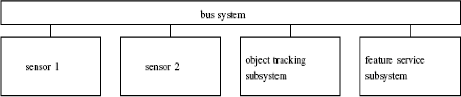
Model of a multi-sensor advanced driver assistance system

3.1. Sensors

In an automotive environment, many obstacle detection systems achieve good results with a combination of active sensors, such as radars and lasers, and passive sensors such as cameras [12]. Thus, sensor 1 is an abstraction of an automotive vision sensor providing position observations, ${\overrightarrow{z}}_1,$ and sensor 2 is an abstraction of an automotive radar or laser sensor providing position and velocity (Doppler) observations, ${\overrightarrow{z}}_2,$ which are calculated with reference to a Cartesian coordinate frame.

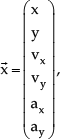
The object state observation vectors can be decomposed into quantities of the true object state vector $\overrightarrow{x}$ mapped by matrix H and a Gaussian distributed error vector $\overrightarrow{r}$ with zero mean [50] as shown in 1 and 2.

${\overrightarrow{z}}_1={\mathrm{H}}_1\cdot \overrightarrow{x}+{\overrightarrow{r}}_1=\left(\begin{array}{l}\mathrm{x}+{\mathrm{r}}_{\mathrm{x},1}\\ \mathrm{y}+{\mathrm{r}}_{\mathrm{y},1}\end{array}\right)$

(1)

${\overrightarrow{z}}_2={\mathrm{H}}_2\cdot \overrightarrow{x}+{\overrightarrow{r}}_2=\left(\begin{array}{l}\mathrm{x}+{\mathrm{r}}_{\mathrm{x},2}\\ \mathrm{y}+{\mathrm{r}}_{\mathrm{y},2}\\ {\mathrm{v}}_{\mathrm{x}}+{\mathrm{r}}_{{\mathrm{v}}_{\mathrm{x}},2}\\ {\mathrm{v}}_{\mathrm{y}}+{\mathrm{r}}_{{\mathrm{v}}_{\mathrm{y}},2}\end{array}\right)$

(2)

The object state observation error covariance matrices, ${\mathrm{R}}_1=\mathrm{E}\left({\overrightarrow{r}}_1,{{\overrightarrow{r}}^{\prime }}_1\right)$ and ${\mathrm{R}}_2=\mathrm{E}\left({\overrightarrow{r}}_2,{{\overrightarrow{r}}^{\prime }}_2\right),$ are assumed to consist of position independent variance values (an example for annotating distance sensor values with variance values is given in [15], particular values for accuracy of vision sensors can be found in [48, 44, 43], for accuracy of radar or laser sensors see [18, 20, 23], for conversion of range and bearing measurements to Cartesian coordinate measurements see [13]).

${\mathrm{R}}_1=\left(\begin{array}{cc}1& \pm 0.001\\ \pm 0.001& 0.01\end{array}\right){\mathrm{m}}^2$

(3)

${\mathrm{R}}_2=\left(\begin{array}{cccc}0.01& \pm 0.001& 0& 0\\ \pm 0.001& 1& 0& 0\\ 0& 0& 0.01\frac{1}{{\mathrm{s}}^2}& \pm 0.001\frac{1}{{\mathrm{s}}^2}\\ 0& 0& \pm 0.001\frac{1}{{\mathrm{s}}^2}& 1\frac{1}{{\mathrm{s}}^2}\end{array}\right){\mathrm{m}}^2$

(4)

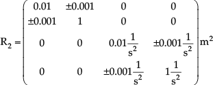
The object state observation error covariance matrices are assumed to be slightly higher than specified in the cited papers. This is due to the fact that the specified precision of both sensors refers to measuring coordinates of points or edges of a non-planar contour of a vehicle.

However, in scenarios where the measured coordinates of points or edges are used for estimating a vehicle's geometrical centre, observations of the vehicle's dimensions, such as width and length, are additionally required [56]. When estimating the vehicle's geometrical centre using width and length observations, the potential inaccuracy of the width and length observations has to be taken into account.

Furthermore, the reflection of a laser scanner or radar beam on a vehicle contour, or the edges that a vision sensor detects when analysing a vehicle contour, may shift during a manoeuvre due to changing aspect angles. This shifting adds further uncertainty to the estimation of the vehicle's geometrical centre and has to be taken into account in the tracking process, for example, by increasing the object state observation error covariance matrices.

The preprocessing times of the sensors are assumed to be dependent on the complexity of the surrounding environment. It is assumed, however, that there are upper bounds for the sensor preprocessing times as each sensor does not detect more than a maximum number of objects. Accordingly, the preprocessing time of sensor 1 is assumed to vary within a range of $\mathrm{c}\cdot$ 160ms to 160ms, and the preprocessing time of sensor 2 is assumed to vary within a range of $\mathrm{c}\cdot$ 80ms to 80ms due to changes in the complexity of the environment [57], where c accounts for different complexity variances.

Furthermore, it is assumed that the sensors do not continuously provide object state observations, but tend to lose an object from time to time, which can result, for example, from object occlusions, difficulties in the observation preprocessing or a badly working association process. The recognition ability is modelled for both sensors independently by a Markov process with binary states $\mathrm{j}=0$ and $\mathrm{j}=1.$

$\overrightarrow{j}=\left(\begin{array}{l}0\\ 1\end{array}\right)$

(5)

where 0 indicates that a sensor has not observed an object and 1 indicates that a sensor has observed an object, the Markov process being governed by the following transition probability matrix.

$\mathrm{J}=\left(\begin{array}{cc}0.975& 0.025\\ 0.01& 0.99\end{array}\right)$

(6)

3.2. Bus System

The bus system within the state-of-the-art model is assumed to be a CAN which operates event-triggered using a carrier sense multiple access/collision resolution scheme. Furthermore, it is assumed that the CAN is exclusively used for transmitting object state observations. The time for transmitting the object state observation vectors from a sensor to the object tracking subsystem is assumed as $\mathrm{\Delta }{\mathrm{t}}_{PT}^{etb}=2\text{\hspace{0.17em}ms}.$

3.3. Object Tracking Subsystem

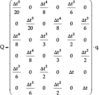
It is further assumed that associated in-sequence object state observations and predicted images of the object states are fused by a Kalman filter algorithm using a white-noise jerk model [51] with

$\overrightarrow{x}=\left(\begin{array}{l}\mathrm{x}\\ \mathrm{y}\\ {\mathrm{v}}_{\mathrm{x}}\\ {\mathrm{v}}_{\mathrm{y}}\\ {\mathrm{a}}_{\mathrm{x}}\\ {\mathrm{a}}_{\mathrm{y}}\end{array}\right),$

(7)

${\mathrm{e}}^{\mathrm{F}\mathrm{\Delta }\mathrm{t}}=\left(\begin{array}{cccccc}1& 0& \mathrm{\Delta }\mathrm{t}& 0& \frac{\mathrm{\Delta }{\mathrm{t}}^2}{2}& 0\\ 0& 1& 0& \mathrm{\Delta }\mathrm{t}& 0& \frac{\mathrm{\Delta }{\mathrm{t}}^2}{2}\\ 0& 0& 1& 0& \mathrm{\Delta }\mathrm{t}& 0\\ 0& 0& 0& 1& 0& \mathrm{\Delta }\mathrm{t}\\ 0& 0& 0& 0& 1& 0\\ 0& 0& 0& 0& 0& 1\end{array}\right)$

(8)

and

$\mathrm{Q}=\left(\begin{array}{cccccc}\frac{\mathrm{\Delta }{\mathrm{t}}^5}{20}& 0& \frac{\mathrm{\Delta }{\mathrm{t}}^4}{8}& 0& \frac{\mathrm{\Delta }{\mathrm{t}}^3}{6}& 0\\ 0& \frac{\mathrm{\Delta }{\mathrm{t}}^5}{20}& 0& \frac{\mathrm{\Delta }{\mathrm{t}}^4}{8}& 0& \frac{\mathrm{\Delta }{\mathrm{t}}^3}{6}\\ \frac{\mathrm{\Delta }{\mathrm{t}}^4}{8}& 0& \frac{\mathrm{\Delta }{\mathrm{t}}^3}{3}& 0& \frac{\mathrm{\Delta }{\mathrm{t}}^2}{2}& 0\\ 0& \frac{\mathrm{\Delta }{\mathrm{t}}^4}{8}& 0& \frac{\mathrm{\Delta }{\mathrm{t}}^3}{3}& 0& \frac{\mathrm{\Delta }{\mathrm{t}}^2}{2}\\ \frac{\mathrm{\Delta }{\mathrm{t}}^3}{6}& 0& \frac{\mathrm{\Delta }{\mathrm{t}}^2}{2}& 0& \mathrm{\Delta }\mathrm{t}& 0\\ 0& \frac{\mathrm{\Delta }{\mathrm{t}}^3}{6}& 0& \frac{\mathrm{\Delta }{\mathrm{t}}^2}{2}& 0& \mathrm{\Delta }\mathrm{t}\end{array}\right)\cdot \mathrm{q}.$

(9)

The time required for fusing all object state observations from one sensor is assumed to be dependent on the complexity of the environment as every additional object increases the required fusion time.

As the maximum number of object state observations is assumed to be restricted, there exists an upper bound for the time required to fuse in-sequence measurements, $\mathrm{\Delta }{\mathrm{t}}_{PT}^{fusISM}\le \mathrm{U}{\mathrm{B}}_{fus}.$ In order to be applicable for typical sensor configuration, the upper bound is assumed to range between 2 ms and 25 ms, $\mathrm{U}{\mathrm{B}}_{fus}=\left\{2,5,10,15,20,25\right\}\text{ms}.$ Furthermore, it is assumed that $\mathrm{\Delta }{\mathrm{t}}_{PT}^{fusISM}$ varies within a range of $\left[\mathrm{c}\cdot \mathrm{U}{\mathrm{B}}_{fus}\right]$ to $\mathrm{U}{\mathrm{B}}_{fus}$ depending on the complexity of the surrounding environment, where c accounts for different complexity variances as modelled in subsection V-A.

The occurrence of out-of-sequence measurements is either dealt with by the BUFF approach (buffering and chronologically sorting measurements) or the ADVA approach as presented by Bar-Shalom in [5]. The ADVA approach is assumed to demand additional processing time following $\mathrm{\Delta }{\mathrm{t}}_{PT}^{fusOOSM}=\lceil \frac{3}{2}\mathrm{\Delta }{\mathrm{t}}_{PT}^{fusISM}\rceil .$

Furthermore, the object tracking subsystem does not maintain buffer object state observations. Newer observations replace older observations from the same sensor. At predefined points in time, the object tracking subsystem starts to predict images of the object states in order to generate real-time images of the object states which are provided to the feature service subsystem. The time required for predicting real-time images of the object states is assumed to be $\mathrm{\Delta }{\mathrm{t}}_{PT}^{pre}=\lceil \frac{1}{3}\mathrm{\Delta }{\mathrm{t}}_{PT}^{fusISM}\rceil .$

The real-time images of the object states are then transmitted to the feature service subsystem. It is assumed that the control loop performed within the feature service subsystem has a frequency of 25Hz, which is a typical value for vehicle control [36, 25, 26].

3.4. State-of-the-art Model Schedule

Figures 3(a) and 3(b) visualize the schedule of the state-of-the-art model for the BUFF or ADVA approach, each process being visualized by a horizontal bar.

Figure 3.

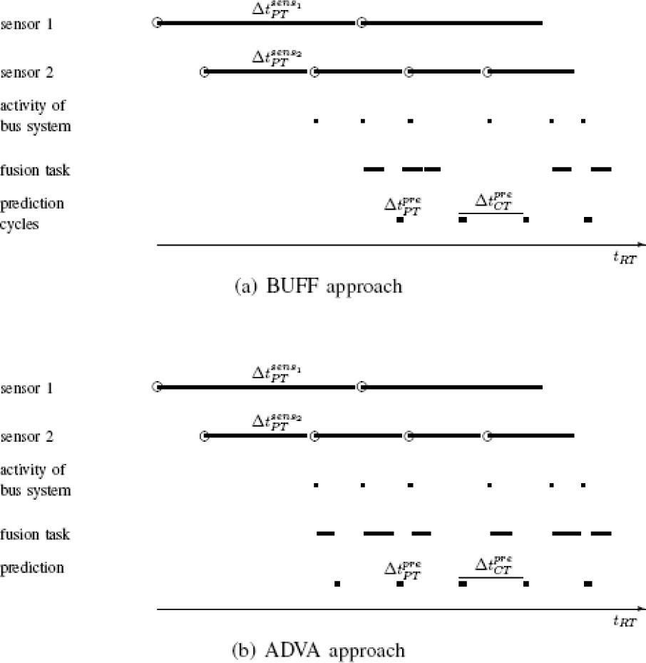
State-of-the-art model schedule

Within the state-of-the-art model as depicted in Figures 3(a) and 3(b), the two sensors (“sensor 1” and “sensor 2”) measure with cycle times, $\mathrm{\Delta }{\mathrm{t}}_{CT}^{sen{\mathrm{s}}_1}$ and $\mathrm{\Delta }{\mathrm{t}}_{CT}^{sen{\mathrm{s}}_2},$ that vary over real-time and are equal to the corresponding sensor preprocessing times, $\mathrm{\Delta }{\mathrm{t}}_{PT}^{sen{\mathrm{s}}_1}$ and $\mathrm{\Delta }{\mathrm{t}}_{PT}^{sen{\mathrm{s}}_2}.$ The sensor preprocessing times are not constant due to the complexity variance as described in subsection V-A. The phases of the sensors are uncontrolled as the internal sensor clocks are not synchronized.

The transmission of an object state observation is indicated in Figure 3(a) and Figure 3(b) by bars labelled “activity of bus system”.

As soon as object state observations are received by the object tracking subsystem and no task is processed simultaneously, the object position observations can be fused with associated images of the object states (“fusion task”) hereby taking into account the particulars of out-of-sequence measurements.

In Figure 3(a), the received object state observations are sorted chronologically within an object state observation buffer which allows the fusion of all object state observations without the use of advanced algorithms. However, as can be seen from Figure 3(a), the buffering of object state observations adds additional delays to the system.

In Figure 3(b), the received object state observations are fused as soon as sufficient processing resources are available. The fusion process task interval, $\mathrm{\Delta }{\mathrm{t}}_{PT}^{fusISM},$ varies as described above.

Every $\mathrm{\Delta }{\mathrm{t}}_{CT}^{pre},$ real-time images of the object states are generated (“prediction cycles”) and transmitted over the bus system to the feature service subsystem.

4. Paradigm shift to time-triggered model

4.1. Sensors

The sensors in a time-triggered multi-sensor advanced driver assistance system are assumed to have fixed sensor cycle times that are equal to the maximum sensor preprocessing times, $\mathrm{\Delta }{\mathrm{t}}_{PT}^{sen{\mathrm{s}}_1}=160\text{\hspace{0.17em}ms}$ and $\mathrm{\Delta }{\mathrm{t}}_{PT}^{sen{\mathrm{s}}_2}=80\text{\hspace{0.17em}ms,}$ i.e., the sensors are scheduled to account for the worst case execution time of observation preprocessing [31]. The sensor phase, $\mathrm{\Delta }{\mathrm{t}}_{PH}^{sen{\mathrm{s}}_2},$ can be controlled and chosen by a system designer in order to arrive at an optimal schedule.

4.2. Bus System

The bus system within the time-triggered model is assumed to be time-triggered using a TDMA scheme, which results in well-defined transmission slots and bounded transmission jitter. $\mathrm{\Delta }{\mathrm{t}}_{CT}^{ttb}$ is chosen to be a factor of $\mathrm{\Delta }{\mathrm{t}}_{CT}^{sen{\mathrm{s}}_1}$ and $\mathrm{\Delta }{\mathrm{t}}_{CT}^{sen{\mathrm{s}}_2},$ and has the typical value of 10ms [17, 24].

The time for transmitting object state observation vectors from a sensor to the object tracking subsystem is assumed to be $\mathrm{\Delta }{\mathrm{t}}_{PT}^{ttb}=2\text{\hspace{0.17em}ms}$ [17].

Please note that the transmission delays introduced by the event-triggered bus system as described in subsection III-B and the time-triggered bus system are assumed to be equal. This assumption seems feasible as the focus of this paper is not on any particular event-triggered or time-triggered bus system, but on the paradigm shift toward time-triggered advanced driver assistance systems.

4.3. Object Tracking Subsystem

The object tracking subsystem fuses the incoming object state observations with associated images of the object states, taking into account the particulars of out-of-sequence measurement processings.

The time-triggered model schedule is set up according to the upper bound for the fusion process task interval $\mathrm{U}{\mathrm{B}}_{fus}$ which is assumed to vary between 2 ms and 25 ms, depending on the hardware resources of the object tracking subsystem.

The occurrence of out-of-sequence measurements is either dealt with by a BUFF approach or an ADVA approach as presented by Bar-Shalom in [5].

At predefined points in time, the object tracking subsystem starts to predict images of the object states in order to generate real-time images of the object states. The scheduling of the prediction can be chosen by a system designer in order to arrive at an optimal schedule.

The real-time images of the object states are then transmitted to the feature service subsystem.

4.4. Time-Triggered Model Schedule

Figures 4(a) and 4(b) depict an unsynchronized time-triggered model schedule for the BUFF approach or the ADVA approach and Figure 5 depicts a synchronized time-triggered model schedule.

Figure 4.

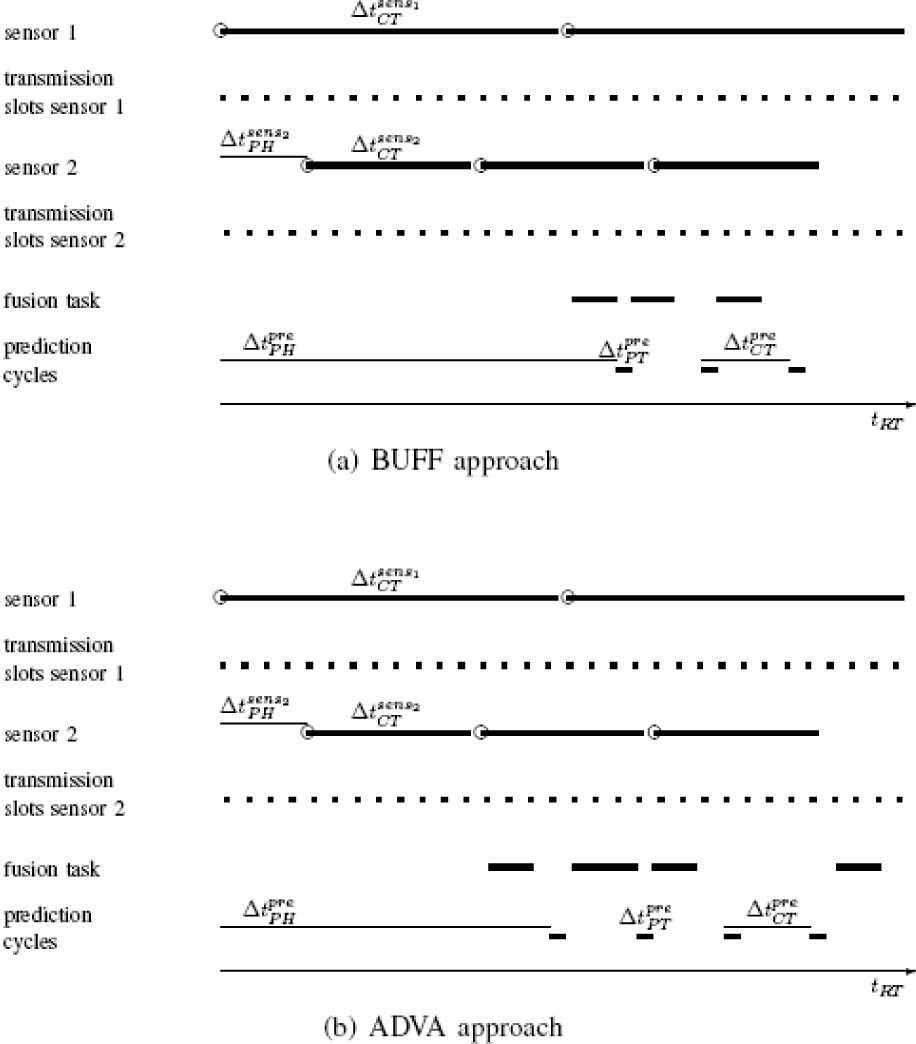
Unsynchronized time-triggered model schedule

Figure 5.

Synchronized time-triggered model schedule points in parameter space

Within the time-triggered model schedules as depicted in Figures 4(a),4(b) and 5, the two sensors have constant cycle times, $\mathrm{\Delta }{\mathrm{t}}_{CT}^{sen{\mathrm{s}}_1}=160\text{\hspace{0.17em}ms}$ and $\mathrm{\Delta }{\mathrm{t}}_{CT}^{sen{\mathrm{s}}_2}=80\text{\hspace{0.17em}ms}$ (observation preprocessing being referred to by the label “sensor 1” respectively “sensor 2”). The phase between sensor 1 and sensor 2 is chosen to be $\mathrm{\Delta }{\mathrm{t}}_{PH}^{sen{\mathrm{s}}_2}=\mathrm{\Delta }{\mathrm{t}}_{CT}^{pre}=40\text{\hspace{0.17em}ms}$ in Figure 4 and $\mathrm{\Delta }{\mathrm{t}}_{PH}^{sen{\mathrm{s}}_2}=0\text{\hspace{0.17em}ms}$ in Figure 5.

The transmission slots of sensor 1 and sensor 2 in Figures 4(a), 4(b) and 5 are scheduled in such a way that the object state observations of sensor 1 are transmitted without any further delay, $\mathrm{\Delta }{\mathrm{t}}_{PH}^{tt{\mathrm{b}}_1}=0,$ and that the object state observations of sensor 2 are transmitted after a delay of 2 ms, $\mathrm{\Delta }{\mathrm{t}}_{PH}^{tt{\mathrm{b}}_2}=2\text{\hspace{0.17em}ms}.$

Please note that in the time-triggered synchronized configuration as depicted in Figure 5, the received object state observations are fused as soon as sufficient processing resources are available, as out-of-sequence measurements are avoided by design.

Every $\mathrm{\Delta }{\mathrm{t}}_{CT}^{pre},$ real-time images of the object states are predicted from the fused images of the object states and then transmitted via the bus system to the feature service subsystem (“prediction cycles”). For the time-triggered unsynchronized ADVA configuration, the prediction cycle phase is

$\mathrm{\Delta }{\mathrm{t}}_{PH}^{pre}=\mathrm{\Delta }{\mathrm{t}}_{PT}^{fusOOSM}+2\cdot \mathrm{\Delta }{\mathrm{t}}_{PT}^{ttb}.$

(10)

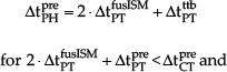
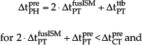
For the time-triggered unsynchronized BUFF configuration, the prediction cycle phase is chosen to be

$\mathrm{\Delta }{\mathrm{t}}_{PH}^{pre}=2\cdot \mathrm{\Delta }{\mathrm{t}}_{PT}^{fusISM}+\mathrm{\Delta }{\mathrm{t}}_{PT}^{ttb}$

(11)

$\text{for\hspace{0.17em}}2\cdot \mathrm{\Delta }{\mathrm{t}}_{PT}^{fusISM}+\mathrm{\Delta }{\mathrm{t}}_{PT}^{pre}\hspace{0.17em}\text{<}\hspace{0.17em}\mathrm{\Delta }{\mathrm{t}}_{CT}^{pre}\hspace{0.17em}\text{and}$

$\mathrm{\Delta }{\mathrm{t}}_{PH}^{pre}=\mathrm{\Delta }{\mathrm{t}}_{PT}^{fusISM}+\mathrm{\Delta }{\mathrm{t}}_{PT}^{ttb}$

(12)

$\text{for\hspace{0.17em}}2\cdot \mathrm{\Delta }{\mathrm{t}}_{PT}^{fusISM}+\mathrm{\Delta }{\mathrm{t}}_{PT}^{pre}\hspace{0.17em}\text{>}\hspace{0.17em}\mathrm{\Delta }{\mathrm{t}}_{CT}^{pre}.$

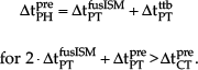
For the time-triggered synchronized configuration, the prediction cycle phase is chosen to be

$\mathrm{\Delta }{\mathrm{t}}_{PH}^{pre}=2\cdot \mathrm{\Delta }{\mathrm{t}}_{PT}^{fusISM}+\mathrm{\Delta }{\mathrm{t}}_{PT}^{ttb}$

(13)

$\text{for\hspace{0.17em}}2\cdot \mathrm{\Delta }{\mathrm{t}}_{PT}^{fusISM}+\mathrm{\Delta }{\mathrm{t}}_{PT}^{pre}\hspace{0.17em}\text{<}\hspace{0.17em}\mathrm{\Delta }{\mathrm{t}}_{CT}^{pre}\hspace{0.17em}\text{and}$

$\mathrm{\Delta }{\mathrm{t}}_{PH}^{pre}=\mathrm{\Delta }{\mathrm{t}}_{PT}^{fusISM}+2\cdot \mathrm{\Delta }{\mathrm{t}}_{PT}^{ttb}$

(14)

$\text{for\hspace{0.17em}}2\cdot \mathrm{\Delta }{\mathrm{t}}_{PT}^{fusISM}+\mathrm{\Delta }{\mathrm{t}}_{PT}^{pre}\hspace{0.17em}\text{>}\hspace{0.17em}\mathrm{\Delta }{\mathrm{t}}_{CT}^{pre}.$

Due to the deterministic nature of the time-triggered approach and the fact that the jitter of all processes is assumed to be sufficiently small compared to the cycle times and can therefore be neglected, the whole system schedule is defined by the constant cycle times and the phases of all processes.

5. Environment model

The environment is modelled with regard to two aspects, the variance of its complexity, i.e., how the preprocessing times of the sensors and the object tracking subsystem depend on the environment, and the process noise which is a measure of how good the employed Kalman filter prediction model describes reality.

5.1. Modelling Environment Complexity

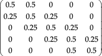
The changes in the complexity of the environment are modelled by a random walk with step size 1 ms. The Markov processes regarding the varying object observation preprocessing times and the varying object observation fusion time are modelled by Markov chains comprising states from $\mathrm{c}\cdot 160\text{\hspace{0.17em}ms}$ to 160 ms, $\mathrm{c}\cdot 80\hspace{0.17em}\text{ms}$ to 80 ms, and $\mathrm{c}\cdot \left\{2,5,\text{\hspace{0.17em}1}0,\text{\hspace{0.17em}15},\text{\hspace{0.17em}2}0,\text{\hspace{0.17em}25}\right\}\text{\hspace{0.17em}ms}$ to $\left\{2,5,\text{\hspace{0.17em}1}0,\text{\hspace{0.17em}15},\text{\hspace{0.17em}2}0,\text{\hspace{0.17em}25}\right\}\text{\hspace{0.17em}ms}.$ For $\mathrm{c}=0.8$ the chain is

$\left(\begin{array}{ccc}\underset{\_}{\mathrm{\Delta }{\mathrm{t}}_{PT}^{sen{\mathrm{s}}_1}/ms}& \underset{\_}{\mathrm{\Delta }{\mathrm{t}}_{PT}^{sen{\mathrm{s}}_2}/ms}& \underset{\_}{\mathrm{\Delta }{\mathrm{t}}_{PT}^{fus}/ms}\\ 128& 64& \left\{2,4,8,12,16,20\right\}\\ 136& 68& \left\{2,5,8,13,17,22\right\}\\ 144& 72& \left\{2,5,9,14,18,23\right\}\\ 152& 76& \left\{2,5,9,14,19,24\right\}\\ 160& 80& \left\{2,5,10,15,20,25\right\}\end{array}\right)$

(15)

with the corresponding state transition probability matrix. ¹

$\left(\begin{array}{ccccc}0.5& 0.5& 0& 0& 0\\ 0.25& 0.5& 0.25& 0& 0\\ 0& 0.25& 0.5& 0.25& 0\\ 0& 0& 0.25& 0.5& 0.25\\ 0& 0& 0& 0.5& 0.5\end{array}\right)$

(16)

5.2. Process Noise

The process noise of the object state evolution is assumed to be white with power spectral density $\mathrm{q},$ and to account for modelling errors, e.g., higher order derivatives that are not contained in the object state vector. In an automotive environment, the choice of a single specific q is problematic since, for example, q in an traffic jam environment will be much smaller than q in a motorway environment.

As a result, q is assumed to vary in the range of $\mathrm{q}=\left[0.01,100\right]\frac{{\mathrm{m}}^2}{{\mathrm{s}}^5}$ to compensate for not modelling the derivative of acceleration in the white noise jerk model of subsection III-C (see also [1, 9, 30, 11]).

6. Performance measure

As mentioned in the introduction, the basis for achieving a correct advanced driver assistance system feature service is a correct assessment of the surrounding environment. The correctness of this assessment depends on the deviations between the real-time images of the object states and reality, which have to be smaller than a feature specific upper bound.

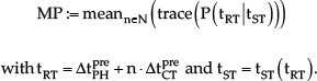
Assuming that all relevant objects are detected by the sensors and that the number of false positives (“ghost” objects) and false negatives (non-detects) is negligible (otherwise the sensors would not be suited for use in advanced driver assistance systems), the mean performance of both models can be expressed by the mean error covariance matrix trace of the real-time images of the object states (for error covariance matrix trace see also [8]). Since the state-time (ST) of the images of the object states is delayed due to object state observation preprocessing, transmission and fusion, it is assumed that the real-time images of the object states are predicted from the state-time images of the object states using the object state evolution model of the Kalman filter, which leads to

$MP:=mea{\mathrm{n}}_{\mathrm{n}\in \mathrm{N}}\left(trace\left(\mathrm{P}\left({\mathrm{t}}_{RT}|{\mathrm{t}}_{ST}\right)\right)\right)$

(17)

$\text{with}\hspace{0.17em}{\mathrm{t}}_{RT}=\mathrm{\Delta }{\mathrm{t}}_{PH}^{pre}+\mathrm{n}\cdot \mathrm{\Delta }{\mathrm{t}}_{CT}^{pre}\text{\hspace{0.17em}and\hspace{0.17em}}{\mathrm{t}}_{ST}={\mathrm{t}}_{ST}\left({\mathrm{t}}_{RT}\right).$

7. Simulation results

We have compared the state-of-the-art and time-triggered configurations for different regions of the parameter space (spanned by the environment parameters and the upper bound for fusion processing time).

7.1. Best Configurations

Figure 6 depicts a three-dimensional parameter space grid spanned by the parameters for complexity variance, $\mathrm{c},$ upper bound for the fusion processing time, $\mathrm{U}{\mathrm{B}}_{fus},$ and process noise power spectral density, $\mathrm{q}.$ Therein, every grid point is identified by a symbol indicating the configuration which is best for the respective parameter set with regard to the simulated mean performance. The symbols are referenced by numbers 1 to 5 in the figure legend, the numbers referring to the model configurations:

Figure 6.

Best state-of-the-art or time-triggered configurations for different

• State-of-the-art BUFF (1);

• State-of-the-art ADVA (2);

• Time-triggered unsynchronized BUFF (3);

• Time-triggered unsynchronized ADVA (4); and

• Time-triggered synchronized (5).

Figure 6 shows that the state-of-the-art ADVA configuration (indicated by blue squares) is best for most grid points in the three-dimensional parameter space grid spanned by complexity variance, upper bound for the fusion processing time, and process noise power spectral density.

However, there are boundary grid points where the state-of-the-art ADVA configuration is outperformed by other configurations.

For big to medium complexity variance in combination with a slow object tracking subsystem and small process noise power spectral density, the state-of-the-art BUFF configuration (indicated by black circles) yields the best results among all possible configurations.

For small complexity variance in combination with a medium-slow to medium-fast object tracking subsystem and medium to high process noise, the time-triggered unsynchronized ADVA configuration (indicated by red triangles) is best.

The time-triggered synchronized configuration (indicated by yellow stars) is best for small complexity variance in combination with a fast or slow object tracking subsystem, and small to high process noise power spectral density.

It is also noteworthy that the time-triggered unsynchronized BUFF configuration is suboptimal over the whole parameter region.

7.2. Best State-of-the-art and Time-Triggered Configurations

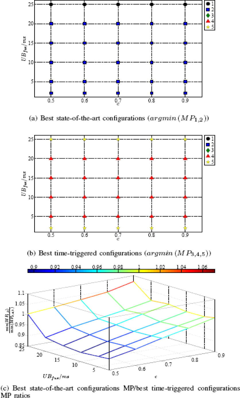
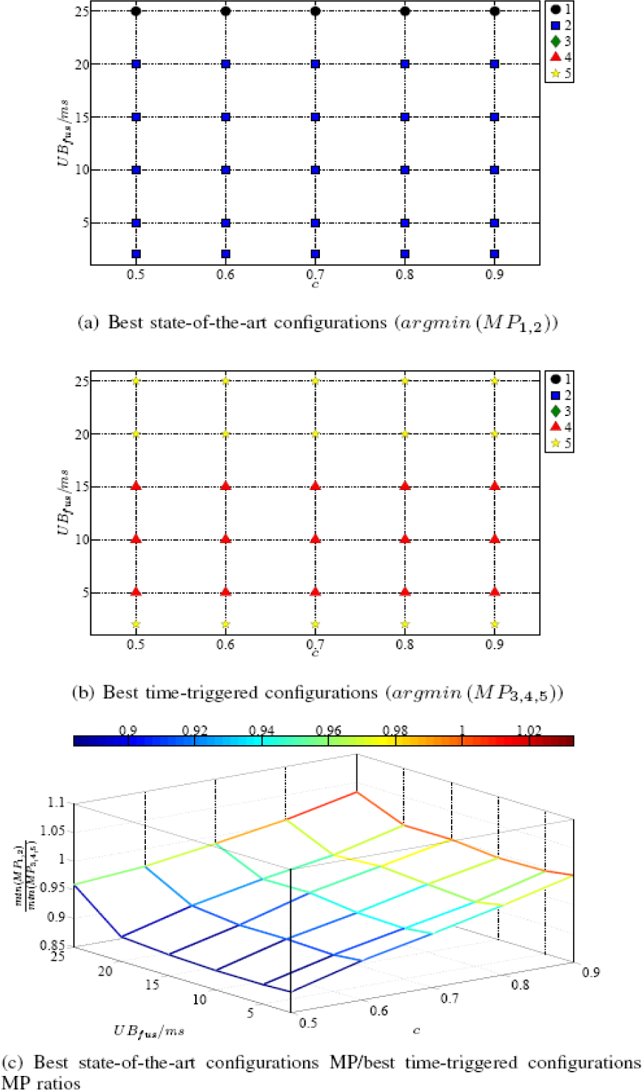
Figures 7, 8, 9, 10 and 11 indicate the best-suited configuration for different parameter ranges and configurations.

Figure 7.

Comparison of best state-of-the-art configurations and best time-triggered configurations for $\mathrm{q}=0.01\frac{{\mathrm{m}}^2}{{\mathrm{s}}^5}$

Figure 8.

Comparison of best state-of-the-art configurations and best timetriggered configurations for $\mathrm{q}=0.01\frac{{\mathrm{m}}^2}{{\mathrm{s}}^5}$

Figure 9.

Comparison of best state-of-the-art configurations and best time-triggered configurations for $\mathrm{q}=1\frac{{\mathrm{m}}^2}{{\mathrm{s}}^5}$

Figure 10.

Comparison of best state-of-the-art configurations and best time-triggered configurations for $\mathrm{q}=1\frac{{\mathrm{m}}^2}{{\mathrm{s}}^5}$

Figure 11.

Comparison of best state-of-the-art configurations and best timetriggered configurations for $\mathrm{q}=100\frac{{\mathrm{m}}^2}{{\mathrm{s}}^5}$

In the top two-dimensional parameter grids, every grid point is identified by a symbol indicating the respective best-suited configuration with respect to the mean performance.

The three-dimensional figures depict the ratio of the best state-of-the-art configurations' mean performance to the best time-triggered configurations' mean performance.

Every set of three subfigures represents one of $\mathrm{q}=0.01\frac{{\mathrm{m}}^2}{{\mathrm{s}}^5},\mathrm{q}=0.1\frac{{\mathrm{m}}^2}{{\mathrm{s}}^5},\mathrm{q}=1\frac{{\mathrm{m}}^2}{{\mathrm{s}}^5},\mathrm{q}=10\frac{{\mathrm{m}}^2}{{\mathrm{s}}^5}$ and $\mathrm{q}=100\frac{{\mathrm{m}}^2}{{\mathrm{s}}^5}.$

Figures 7(a),8(a), 9(a), 10(a) and 11(a) show that the state-of-the-art BUFF configuration outmatches the state-of-the-art ADVA configuration for slow object tracking subsystems, $\mathrm{U}{\mathrm{B}}_{fus}=25\text{\hspace{0.17em}ms,}$ in combination with small to medium process noise power spectral density, $\mathrm{q}=\left\{0.01,0.1,1\right\}\frac{{\mathrm{m}}^2}{{\mathrm{s}}^5}.$ However, for the remaining parameter grid points, the state-of-the-art ADVA configuration yields better results than the state-of-the-art BUFF configuration.

Regarding the time-triggered configurations, Figures 7(b),8(b), 9(b), 10(b) and 11(b) show that for medium upper bound for the fusion processing time, $\mathrm{U}{\mathrm{B}}_{fus}=\left\{5,10,15\right\}\text{ms}$ in combination with small process noise power spectral density, $\mathrm{q}=\left\{0.01,0.1\right\}\frac{{\mathrm{m}}^2}{{\mathrm{s}}^5},$ the time-triggered unsynchronized ADVA configuration outmatches the time-triggered synchronized configuration and the time-triggered unsynchronized BUFF configuration. For the other upper bounds for the fusion processing time, $\mathrm{U}{\mathrm{B}}_{fus}=\left\{2,20,25\right\}\text{ms}.$ however, the time-triggered synchronized configuration outmatches the time-triggered unsynchronized ADVA configuration and the time-triggered unsynchronized BUFF configuration.

With increasing process noise power spectral density, $\mathrm{q}=\left\{1,10\right\}\frac{{\mathrm{m}}^2}{{\mathrm{s}}^5},$ the time-triggered unsynchronized ADVA configuration outmatches the time-triggered synchronized configuration also for the upper bound of the fusion processing time of $\mathrm{U}{\mathrm{B}}_{fus}=\left\{20\right\}\text{ms,}$ i.e., the best time-triggered configuration for $\mathrm{U}{\mathrm{B}}_{fus}=20\hspace{0.17em}\text{ms}$ shifts from the time-triggered synchronized configuration to the time-triggered unsynchronized ADVA configuration.

For high process noise power spectral density, $\mathrm{q}=100\frac{{\mathrm{m}}^2}{{\mathrm{s}}^5},$ the time-triggered unsynchronized ADVA configuration outmatches the time-triggered synchronized configuration for medium to high upper bounds for the fusion processing time, $\mathrm{U}{\mathrm{B}}_{fus}=\left\{10,15,20,25\right\}\text{ms,}$ and the time-triggered synchronized configuration outmatches the time-triggered unsynchronized ADVA configuration for a fast object tracking subsystem, $\mathrm{U}{\mathrm{B}}_{fus}=\left\{2,5\right\}\text{ms}.$ This shows that if the process noise power spectral density increases from $\mathrm{q}=10\frac{{\mathrm{m}}^2}{{\mathrm{s}}^5}$ to $\mathrm{q}=100\frac{{\mathrm{m}}^2}{{\mathrm{s}}^5},$ the best time-triggered configuration shifts from the time-triggered unsynchronized ADVA configuration to the time-triggered synchronized configuration for an upper bound of the fusion processing time of $\mathrm{U}{\mathrm{B}}_{fus}=5\hspace{0.17em}\text{ms}.$ For an upper bound of the fusion processing time of $\mathrm{U}{\mathrm{B}}_{fus}=25\hspace{0.17em}\text{ms,}$ however, the best time-triggered configuration shifts vice versa.

Regarding the mean performance of the best state-of-the-art configurations and the best time-triggered configurations, Figures 7(c),8(c), 9(c), 10(c) and 11(c) show the mean performance ratios of the best state-of-the- art configurations to the best time-triggered configurations which have been identified in Figures 7(a),8(a), 9(a), 10(a), 11(a), 7(b), 8(b), 9(b), 10(b) and 11(b). The figures show that the difference between the best state-of-the-art configurations and the best time-triggered configurations range from −15% to +6% of the mean real-time error covariance matrix trace of the respective best time-triggered configuration.

For low process noise power spectral density, $\mathrm{q}=0.01\frac{{\mathrm{m}}^2}{{\mathrm{s}}^5},$ the difference ranges from −15% to +1% and for high process noise power spectral density, $\mathrm{q}=100\frac{{\mathrm{m}}^2}{{\mathrm{s}}^5},$ the difference ranges from −10% to +2%. It should be noted however, that the biggest difference of +6% is found for medium process noise power spectral density, $\mathrm{q}=1\frac{{\mathrm{m}}^2}{{\mathrm{s}}^5}.$

8. Analysis of simulation results

As the time-triggered configurations schedule all processes in accordance with their worst case execution time, the mean performance measures of the time-triggered model configurations are unaffected by a decrease of the lower bounds for sensor and fusion preprocessing times, indicated by a decrease of the complexity variance parameter. As a state-of-the-art configuration may start a new task as soon as the preceding task has been finished, the state-of-the-art configuration profit from shorter sensor and fusion preprocessing times. This leads to the observed behaviour where the state-of-the-art configurations outmatch the time-triggered configurations for a decreasing complexity variance parameter, as shown in Figures 7(c),8(c), 9(c), 10(c) and 11(c).

The time-triggered synchronized configuration is able to fuse all object state observations, but is more valuable in the sequence of intervals between state-time and real-time compared to the state-of-the-art ADVA configuration. Accordingly, an increase in the process noise power spectral density which increases the sequence of integrated process noise traces to a greater extent than the sequence of object state state-time image error covariance matrix traces is unfavourable for the time-triggered synchronized configuration, as the time-triggered synchronized configuration has the greater values in the sequence of intervals between state-time and real-time and therefore, the sequence of greater integrated process noise traces. The reason why the state-of-the-art ADVA configuration is outmatched by the time-triggered synchronized configuration for medium process noise power spectral density lies in the fact that the state-of-the-art ADVA configuration cannot fuse all object state observations of sensor 1. When the process noise power spectral density decreases, the influence of the integrated process noise traces is diminished and the focus shifts toward the sequence of object state state-time image error covariance matrix traces. Here, the state-of-the-art BUFF configuration outmatches the time-triggered synchronized configuration due to the higher number of object state observation sets that are fused. The reason why this behaviour is also observed for small lower bounds for sensor and fusion preprocessing times is obvious when considering that the long times required to fuse an object state observation set and the high number of uncoordinated object state observation sets may lead to fusion “jams”.

The time-triggered unsynchronized ADVA configuration has a sequence of object state state-time image error covariance matrix traces that is unaffected by a variation in the upper bound for the fusion processing time, but reacts with a 1.5 times greater variation in the sequence of intervals between state-time and real-time. The time-triggered synchronized configuration experiences a jump in the sequence of object state state-time image error covariance matrix traces for the upper bound for the fusion processing time changing from $\mathrm{U}{\mathrm{B}}_{fus}=15\hspace{0.17em}\text{ms}$ to $\mathrm{U}{\mathrm{B}}_{fus}=20\hspace{0.17em}\text{ms}.$ Furthermore, the sequence of intervals from state-time to real-time varies proportionally for $\mathrm{U}{\mathrm{B}}_{fus}\ge 20\hspace{0.17em}\text{ms}$ and twice as great for $\mathrm{U}{\mathrm{B}}_{fus}\le 15\hspace{0.17em}\text{ms}.$ Accordingly, the sequence of intervals between state-time and real-time increases stronger in the time-triggered synchronized configuration for the upper bound for the fusion processing time $\mathrm{U}{\mathrm{B}}_{fus}\le 15\hspace{0.17em}\text{ms}$ and weaker for $\mathrm{U}{\mathrm{B}}_{fus}\ge 20\hspace{0.17em}\text{ms}$ than the time-triggered unsynchronized configuration, which leads to the observed behaviour.

The observed interrelation derives from the influence of the sequence of integrated process noise traces that increase with increasing process noise power spectral density. In this regard, the jump in sequence of object state state-time image error covariance matrix traces which react unfavourably to the upper bound for the fusion processing time changing from $\mathrm{U}{\mathrm{B}}_{fus}=15\hspace{0.17em}\text{ms}$ to $\mathrm{U}{\mathrm{B}}_{fus}=20\hspace{0.17em}\text{ms}$ becomes greater and makes it impossible for the time-triggered synchronized configuration to be competitive.

9. Conclusion

In this paper a state-of-the-art model and a time-triggered model for multi-sensor advanced driver assistance systems have been compared. In the state-of-the-art model, the sensor phases are not controllable and the sensor cycle times are equal to the sensor preprocessing times which vary within a given range according to a Markov chain with given transition probability matrix. The state-of-the-art model can be operated in two configurations, a state-of-the-art BUFF configuration, where object state observations are buffered and chronologically sorted before fusion, and a state-of-the-art ADVA configuration that directly fuses out-of-sequence measurement using an ADVA approach.

In the time-triggered model, the sensor phases are controllable, the sensor cycle times are fixed and equal to the sensors' worst case preprocessing times. Furthermore, a time-triggered bus system with fixed transmission slots is used that transmits the object position observations from the sensors to the object tracking subsystem. The time-triggered model can be operated in various configurations from which three phase-aligned configurations are selected for further analysis: a time-triggered unsynchronized BUFF configuration, a time-triggered unsynchronized ADVA configuration, and a time-triggered synchronized configuration, where the object state observation sampling of both sensors is either unsynchronized or synchronized.

The mean performance of both models has been evaluated by simulations with multiple configurations differing in the sensor and bus system schedules, and the treatment of OOSMs. The results show that for the chosen parameter space, the state-of-the-art ADVA configuration yields the best results. However, the results also show that there are points in parameter space where the state-of-the-art ADVA configuration is outmatched by the state-of-the-art BUFF configuration, the time-triggered unsynchronized ADVA configuration or the time-triggered synchronized configuration.

Accordingly, the state-of-the-art configurations are favourable when the sensor preprocessing times show very high variations. However, with decreasing sensor preprocessing time variation, the time-triggered configurations outmatch the state-of-the-art configurations for two reasons. The first reason is the increasing mean of the sequence between state-time to real-time. The second reason is that the time-triggered configurations show a smaller variation in the sequence between state-time and real-time which is advantageous when considering the higher order dependence of the mean trace of the integrated process noise. As a result, the state-of-the-art configurations show weaknesses in situations of high risk potential, because such situations are characterized by a high number of objects which leads to low sensor preprocessing time variation and/or a fast changing environment which is represented by a high process noise power spectral density.

Given the aforesaid, it can be concluded that time-triggered control paradigm is well-suited for advanced driver assistance systems equipped with sensors of the current generation, as positive features like guaranteed accuracy intervals, bounded detection latency for timing and omission errors, replica determinism and temporal composability are achieved by a minimal degradation of the mean system performance.