Experimental Study of the Methodology for the Modelling and Simulation of Mobile Manipulators

Abstract

This paper describes an experimental study of a novel methodology for the positioning of a multi-articulated wheeled mobile manipulator with 12 degrees of freedom used for handling tasks with explosive devices. The approach is based on an extension of a homogenous transformation graph (HTG), which is adapted to be used in the kinematic modelling of manipulators as well as mobile manipulators. The positioning of a mobile manipulator is desirable when: (1) the manipulation task requires the orientation of the whole system towards the objective; (2) the tracking trajectories are performed upon approaching the explosive device's location on the horizontal and inclined planes; (3) the application requires the manipulation of the explosive device; (4) the system requires the extension of its vertical scope; and (5) the system is required to climb stairs using its front arms. All of the aforementioned desirable features are analysed using the HTG, which establishes the appropriate transformations and interaction parameters of the coupled system. The methodology is tested with simulations and real experiments of the system where the error RMS average of the positioning task is 7. 91 mm, which is an acceptable parameter for performance of the mobile manipulator.

1. Introduction

Mobile manipulators exhibit wide versatility in the handling of dangerous devices, such as the explosive ordinance devices (EOD) used by the world's armies. Among the most important phases in the mechatronic design of mobile manipulators we have modelling and simulation, because upon them depends the proposed control for its correct operation and the fact that its behaviour will be verified by the simulation of several instances in order to obtain the parameters and ranks from the mobile manipulator that is being developed.

In relation to the modelling of mobile manipulators, the work of Yamamoto, Alicja Mazur and Bayle is well known. Yamamoto is the most cited, with his paper on the locomotion coordination of mobile manipulators, published in 2004. Alicja Mazur and Bayle are the authors that have written most in relation to this topic. Since 1976, there are records of works related to the programming of teleoperated mobile manipulators [1]; moreover, in 1988 [2] and 1996 [3–4], the dynamics of mobile manipulators in the operational case of the opening of a door was proposed; however, the manipulator and the mobile platform were considered and analysed separately. Besides this, from 1994 to 2008, some works were published on mobile manipulators with planar manipulators but without considering the load or other operational cases; they were focused only on control, kinematic redundancy, tracking trajectories and manipulability [5, 18, 26, 29].

In order to obtain the modelling of mobile manipulators used in the tasks for positioning in the handling and transport of explosive devices, the present work considers the development of a modelling methodology for mobile manipulators by applying the mechatronic design of a multi-articulated wheeled mobile manipulator called Robot MMR12-EOD. Unlike the others methodologies presented in previous works, it considers the problem of the mechatronic design, the coupled full system and kinematic modelling in real operations. An experimental study of the methodology capable of performing this positioning in real operational scenarios is described throughout this paper.

The rest of the paper is organized as follows. Section 2 describes the methodology for the kinematic modelling of the full system and the experiments in several scenarios of operation. Later, Section 3 presents the results in which the basis of the reference values that were obtained in the modelling are presented with the errors from the simulation and the real experiment, comparing them with the ideal parameters and both errors. This work is discussed and is concluded in Sections 4 and 5, respectively.

2. Modelling and Simulation Methodology

This section presents the modelling methodology for wheeled mobile manipulators, describing the planning, development and experimentation. It is organized as follows: preliminary analysis, master map, diagram of position and orientation, homogenous transformation graph, kinematic schemes of operation scenarios, kinematic interactions, forward and inverse kinematic, constraints, dynamic parameters, consolidation of the dynamic equation, real experimentation and positioning simulation.

2. 1 Preliminary analysis

The robot MMR12-EOD is considered by being able to move on a surface by the action of its wheels mounted in the robot and touching the surface. The wheels are mounted on devices that allow relative movement between its attached point (point of guidance) and a surface (the floor), at which it must have a unique rolling contact [6–7]. It is assumed that the robot is being built with rigid mechanisms, that there is an link guided by every wheel, that all the axes guided are perpendicular to the floor, that the surface of the motion is a plane, and that there is no sliding with the rolling surface and that the friction is sufficiently small to allow the rotation of any wheel about the guided axis [8–10]. Sliding with the surface is the biggest problem during the moment of establishing a location with high accuracy. Figure 1 shows that the mobile platform has 4-DOF, that the manipulator has 4-DOF and that the added subsystem does too.

Figure 1.

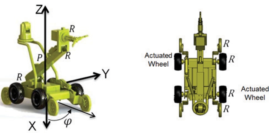
Robot MMR12-EOD

The average velocity of the robot MMR12-EOD is 0. 5 m/s and it is required to support a load of 10 kg at its end effector. These features, as well as the critical parameters and the kind of system (non-holonomic) are used as a base in order to form the master map.

2. 2 Master map

The master map is a diagram that shows the development of the mathematical model, in which is represented the subsystems and homogenous transformations of the mobile manipulator. Described first are both the external and internal constraints, being those external constraints which are related to the operating environment. As such, the terrain is considered as the localization of its local coordinates with respect to global coordinates. The internal constraints are determined according to the non-holonomy of the mobile platform. Afterwards, the scheme with the nomenclature M-MMR (adding the other subsystem) is classified, where M is the manipulator and MMR is the mobile to which is added the other subsystem, like the lifting arms or any subsystem. In the case where the additional subsystem is a manipulator (operating cooperatively and located in the same origin as that of the principal manipulator), then the homogenous transformations of this subsystem will relate to the origin coordinate “0” rather than being related to the local coordinate “C”. The master map has the stages related to the subsystems for the mobile manipulator MMR12-EOD in relation to the tasks of orientation, approaching and manipulation; in this case, the mobile manipulator has an added subsystem formed by two coupled lifting arms (B. A.) at which are considered the lifting and climbing tasks [11–14]. In order to model the robot MMR12-EOD, seven stages in five real operation scenarios are considered [7], at which the assessed behaviour of the full system with and without load is considered. For the robot in the present work, the stages are:

• a)

The additional subsystem is considered in the neutral position and in operation with respect to the local coordinate “C”. This subsystem is called “A”. This stage is omitted if the manipulator has no additional subsystem.

b)

The manipulator uses just its degrees of freedom to perform tracking trajectories tests in relation to the coordinate “0”, which is the base of the manipulator.

c)

The mobile platform is moved forward with the manipulator mounted and performing a tracking trajectory test from the coordinate “C” to the global coordinate “G4”.

d)

Considering the coupled system without allowing the advance of the mobile platform, the manipulator realizes the test of the tracking trajectory, assuming that the mobile platform rotates about its axis with respect to the local coordinate “C”.

e)

The mobile platform is moved forward with the manipulator coupled while performing a tracking trajectory test from the coordinate “C” with respect to the global coordinate “G4”.

f)

The coupled system is moved in a straight line, moving its manipulator in relation to the end effector with respect to “G4”.

g)

The coupled system is subjected to the tests for tracking the trajectory in relation to the end effector with respect to the coordinate “G4”.

2. 3 Diagram of the position and orientation

The general description for the orientation and position of the system is described by the fourth transformation of the global coordinates with respect to GG, as shown in Figure 2.

Figure 2.

Fourth Transformation of the global coordinates with respect to the global coordinates

2. 4 Homogeneous transformation graph (HTG)

The third step of the proposed methodology is the homogenous transformation graph that, in a modular way, allows the organization of the subsystems that constitute the mobile manipulator plus the added subsystem. This graph is an extension of the graph for obtaining the kinematics of the manipulators proposed by Robert Pauli, in 1983 [15], and used in several works by Tadeusz Skodny [16, 30] in order to perform the same applications. The extension of Pauli's graph allows us to get the homogenous transformation graph and the kinematic modelling of wheeled mobile manipulators with any additional subsystem. These transformations are the central part of the methodology because they provide the relations with the coordinates “0” of manipulator and “C” of the mobile platform, as well as the transformations of the wheels and the lifting arms in relation to “C” and “C” with respect to “G4”, as shown in Figure 3. Afterwards, coordinates systems to the selected points that allow us to obtain the coupled kinematic modelling of full system are assigned.

Figure 3.

HTG for mobile manipulators

2. 5 Schemes for the kinematics of the operation scenarios

In order to realize the schemes for the kinematics of five real operational scenarios of the MMR12-EOD robot, it is necessary to consider its design parameters.

2. 6 Interaction kinematics

Table 2 presents the parameters of the interaction kinematics obtained from the coupling of the subsystems of the robot MMR12-EOD.

Table 1.

Constraint equations to the robot MMR12-EOD

The mobile platform must move in the direction of its axis of symmetry with respect to the ground, where (xco, yco, zco) are the coordinates of its centre of mass and φ is the heading angle of the platform measured from xG(4) [26].	${\stackrel{.}{\mathrm{y}}}_{\text{co}}cos\phi -{\stackrel{.}{\mathrm{x}}}_{\text{co}}sin\phi =0$ (12)
The other two constraints are the rolling constraints – i. e., the driving wheels do not slip -where θr, θ1] are the angular displacements of the right and left wheels, respectively [26].	${\dot{x}}_{Co}cos\phi +{\dot{y}}_{Co}sin\phi +\dot{\phi }b={\dot{\theta }}_{r}r$ (13) $\dot{\phi }=\frac{r}{2b}({\dot{\theta }}_r-{\dot{\theta }}_1)$ (14)

Table 2.

Tasks for orientation and the tracking trajectory

Tracking trajectory about its geometric centre.	Sampling time: tm = 200 s. The reference C is located on these coordinates: $\begin{array}{c}y\hspace{0.17em}\mathit{desired}=0\\ x\hspace{0.17em}\mathit{desired}=0\end{array}$ Mean error of 40 mm.
Tracking trajectory of the sinusoidal curve.	tm = 200 s. The reference is located on these curves: $\begin{array}{c}y\hspace{0.17em}\mathit{desired}=30\hspace{0.17em}sen\hspace{0.17em}(0.25\hspace{0.17em}t)\\ x\hspace{0.17em}\mathit{desired}=40\hspace{0.17em}cos(0.25\hspace{0.17em}t)+2.5\hspace{0.17em}t\end{array}$ Mean error of 2. 37 mm.

2. 7 Forward and inverse kinematics

2. 7. 1 Forward kinematics

Based on the homogenous transformation graph and the table of the kinematic interactions, we develop the forward kinematics, starting with the coordinate “C”, and from here describe the transformations of the wheels, the lift arms and the manipulator, considering the end effector “E” with the load “Eμ”, as shown in figures 4 and 6 [17, 28–30].

Figure 4.

Lateral view of the MMR12-EOD in the lifting position

Figure 5.

Scheme for the inverse kinematics

Figure 6.

Mobile manipulator in a real experiment

a) Mobile platform

The homogenous transformation of the mobile platform is given by 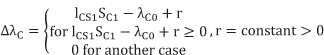${\mathrm{A}}_{\mathrm{C}}=\left({\mathrm{x}}_{\mathrm{G}}^{\left(4\right)}{\mathrm{y}}_{\mathrm{G}}^{\left(4\right)}{\mathrm{z}}_{\mathrm{G}}^{\left(4\right)}\to {\mathrm{x}}_{\mathrm{C}}{\mathrm{y}}_{\mathrm{C}}{\mathrm{z}}_{\mathrm{C}}\right)$ , where the parameters are: A_C:x_C0 = var, y_C0 = var, z_C = var = λ._C0 + δ_C, z_C0 = λ._C0 = const > 0, θ_C1 = var, l_CS1 = const > 0, φ = var. The increment of λ_C depends upon the following relationship:

${\Delta \mathrm{\lambda }}_{\mathrm{C}}=\left\{\begin{array}{c}{\mathrm{l}}_{\mathrm{C}\mathrm{S}1}{\mathrm{S}}_{\mathrm{C}1}-{\mathrm{\lambda }}_{\mathrm{C}0}+r\\ for {\mathrm{l}}_{\mathrm{C}\mathrm{S}1}{\mathrm{S}}_{\mathrm{C}1}-{\mathrm{\lambda }}_{\mathrm{C}0}+r\ge 0\\ 0 \text{for another case}\end{array}\right.,\mathrm{ }\mathrm{r}=\mathrm{c}\mathrm{o}\mathrm{n}\mathrm{s}\mathrm{t}\mathrm{a}\mathrm{n}\mathrm{t}>0$

(1)

Then the transformation of the local coordinate, GT_C = A_C and the transformations for the wheels of the right side and the left side, GT_R = A_CA_R and GT_L = A_CA_L are obtained[29–30].

b) Lifting arms

The transformations of the lifting arms are developed with respect to the local coordinate “C”. The parameters for the lifting arm of the right front side are given by: A_CS1: θ_CS1 = var, l_CS1 = const > 0. Therefore, the transformation of first arm in relation to the global coordinates is expressed as GT_CS1 = A_CA_C1A_CS1. In a similar way, the relations for the second, third and fourth lifting arms are obtained.

c) Manipulator

The homogenous transformations of its 4-DOFs with respect to the coordinate “0” in relation to the coordinate “C” are now presented. The homogeneous transformation from “C” to “0”, A₀ = (x_Cy_Cz_C → x₀y₀z₀), depends upon the following parameters: θ₀ = 0°, λ₀ = const > 0,1₀ = const < 0 α₀ = 90°. The transformation A₁ = (x₀y₀z₀ → x₁y₁z₁), depends upon the following parameters: θ₁ = var, λ₁ = 0, l₁ = 0 α₁ = 90°. The transformation A₂ = (x₁y₁z₁ → x₂y₂z₂), depends upon the following parameters: θ₂ = 0°, λ₂ = var, l₂ = 0 α₂ = −90°. The transformation A₃ = (x₂y₂z₂ → x₃y₃z₃) depends upon the following parameters: θ₃ = var, λ₃ = 0, l₃ = const > 0, α₃ = 90° and the transformation A₄ = (x₃y₃z₃ → x₄y₄z₄) depends upon the following parameters:: θ₄ = var, λ₄ = 0,l₄ = 0 α₄ = 0°.

The transformations of the end effector in relation to the fourth degree of freedom of the manipulator are given by E = (x₄y₄z₄ → x₅y₅z₅), where E = Trans(0,0, λ₅) and its parameters are E: θ₅ = 0°, λ₅ = const > 0, l₅ = 0 α₅ = 0°. In order to obtain transformations that connect the load with the end effector, these are obtained by the relationship E_μ = E_μ-P E_μ-R, where E_μ is the total load, constituted byE_μ-P y E_μ-R, which are the prismatic load and the rotational load, respectively [18]. The parameters of the prismatic joint are as follows: E_μ-P: θ₆ = 0°, λ₆ = const > 0, l₆ = 0 α₆ = 0°. The parameter of the rotational joint are as follows: E_μ-R: θ₇ = 0°, λ₇ = 0, l₇ = 0 α₇ = 90°.

Then, the transformations from the joints of the manipulator are multiplied so that the transformation of the manipulator is T₄, using the trigonometric simplification Cos(A + B) = C_AC_B – S_AS_B = C_AB,. Sen(A + B) = C_AS_B + S_AC_B = S_AB is obtained by the transformation from the manipulator to the global coordinates given by GT₄ = A_CCT₄. The transformation of the end effector with the load is determined by = E_μ-P E_μ-R. Finally, we obtain the homogeneous transformation from the load “X” in the end effector in relation to the global coordinates described by equation 2 [19].

$\begin{array}{c}{\mathrm{X}}_{\mathrm{M}}=\mathrm{G}\mathrm{ }{\mathrm{T}}_4\mathrm{E}{\mathrm{ }\mathrm{E}}_{\mathrm{\mu }}=\\ \left[\begin{array}{cccc}\mathrm{A}& D& \mathrm{G}& {\mathrm{x}}_{\mathrm{C}}+{\mathrm{C}}_{\mathrm{C}}({\mathrm{S}}_1{\mathrm{\lambda }}_2+{\mathrm{l}}_3{\mathrm{C}}_{13}-{\mathrm{l}}_0)+{\mathrm{C}}_{\mathrm{C}}{\mathrm{\lambda }}_5{\mathrm{S}}_{13}+{\mathrm{C}}_{\mathrm{C}}{\mathrm{\lambda }}_6{\mathrm{S}}_{13}\\ B& E& H& {\mathrm{y}}_{\mathrm{C}}+{\mathrm{S}}_{\mathrm{C}}({\mathrm{S}}_1{\mathrm{\lambda }}_2+{\mathrm{l}}_3{\mathrm{C}}_{13}-{\mathrm{l}}_0)+{\mathrm{S}}_{\mathrm{C}}{\mathrm{\lambda }}_5{\mathrm{S}}_{13}+{\mathrm{S}}_{\mathrm{C}}{\mathrm{\lambda }}_6{\mathrm{S}}_{13}\\ \mathrm{C}& F& I& {\mathrm{z}}_{\mathrm{C}0}+{\Delta \mathrm{\lambda }}_{\mathrm{C}}+{\mathrm{\lambda }}_0-{\mathrm{\lambda }}_5{\mathrm{C}}_{13}-{\mathrm{C}}_1{\mathrm{\lambda }}_2+{\mathrm{l}}_3{\mathrm{S}}_{13}-{\mathrm{\lambda }}_6{\mathrm{C}}_{13}\\ 0& 0& 0& 1\end{array}\right]\end{array}$

(2)

where:

$\begin{array}{c}A={\mathrm{S}}_4{\mathrm{S}}_{\mathrm{C}}+{\mathrm{C}}_{\mathrm{C}}{\mathrm{C}}_{13}{\mathrm{C}}_4,\mathrm{ }B={\mathrm{S}}_{\mathrm{C}}{\mathrm{C}}_{13}{\mathrm{C}}_4-{\mathrm{C}}_{\mathrm{C}}{\mathrm{S}}_4,\mathrm{ }C={\mathrm{S}}_{13}{\mathrm{C}}_4,\mathrm{ }D=\\ {\mathrm{C}}_{\mathrm{C}}{\mathrm{S}}_{13},\mathrm{ }E={\mathrm{S}}_{\mathrm{C}}{\mathrm{S}}_{13},\mathrm{ }F=-{\mathrm{C}}_{13},\mathrm{ }G={\mathrm{C}}_{\mathrm{C}}{\mathrm{C}}_{13}{\mathrm{S}}_4-{\mathrm{C}}_4{\mathrm{S}}_{\mathrm{C}},\mathrm{ }H=\\ {\mathrm{S}}_{\mathrm{C}}{\mathrm{C}}_{13}{\mathrm{S}}_4+{\mathrm{C}}_4{\mathrm{C}}_{\mathrm{C}},\mathrm{ }I={\mathrm{S}}_{13}{\mathrm{S}}_4\end{array}$

2. 7. 2 Inverse kinematics

Here, the equations that connect the Cartesian coordinates of the task space in relation to the joint parameters are described in order to carry the end effector from the mobile manipulator to the mentioned Cartesian coordinates. The inverse kinematics were developed using the homogeneous transformations of the equations 3 to 11 from the scheme for forward and the inverse kinematics, which is represented by Figure 5.

$\mathrm{\phi }={\mathrm{t}\mathrm{a}\mathrm{n}}^{-1}\left(\frac{\mathrm{d}\mathrm{y}}{\mathrm{d}\mathrm{x}}\right)$

(3)

${\mathrm{\theta }}_3={\mathrm{c}\mathrm{o}\mathrm{s}}^{-1}\left[\frac{{\mathrm{d}\mathrm{x}}^2{+\mathrm{d}\mathrm{y}}^2+{\mathrm{d}\mathrm{z}}^2{{-\mathrm{\lambda }}_2}^2{{-\mathrm{\lambda }}_5}^2}{{-2\mathrm{ }\mathrm{\lambda }}_2{\mathrm{ }\mathrm{\lambda }}_5}\right]$

(4)

${\mathrm{ }\mathrm{\lambda }}_2=\frac{{\mathrm{ }\mathrm{d}}_{\mathrm{Z}}+{\mathrm{ }\mathrm{\lambda }}_0-{\mathrm{ }\mathrm{\lambda }}_5{\mathrm{ }\mathrm{C}}_3+{\mathrm{ }\mathrm{l}}_3{\mathrm{ }\mathrm{S}}_3}{{\mathrm{ }\mathrm{C}}_3}$

(5)

$\mathrm{E}={\mathrm{t}\mathrm{a}\mathrm{n}}^{-1}\left(\frac{{\mathrm{l}}_3}{{\mathrm{\lambda }}_5}\right);\mathrm{ }\mathrm{K}=180-90-\mathrm{E}1;\mathrm{ }\mathrm{h}=\left(\frac{{\mathrm{l}}_3}{{\mathrm{S}}_{\mathrm{E}}}\right);$

(6)

$\mathrm{P}=180-\mathrm{K}-{\mathrm{q}}_3;\mathrm{ }\mathrm{r}=\sqrt{{\mathrm{h}}^2+{\mathrm{d}}_2^2-\left[2\mathrm{h}{\mathrm{d}}_2{\mathrm{C}}_{\mathrm{P}1}\right]}\mathrm{ };$

(7)

$\mathrm{d}={\cos }^{-1}\left(\frac{\left({\mathrm{h}}^2+{\mathrm{r}}^2-{\mathrm{d}}_2^2\right)}{2\mathrm{h}\mathrm{r}}\right);{\mathrm{q}}_1^{\mathrm{\text{'}}}=180-\mathrm{P}-\mathrm{d}1;$

(8)

${\mathrm{q}}_1^{\mathrm{\text{'}}\mathrm{\text{'}}}={\mathrm{sen}}^{-1}\left(\frac{{\mathrm{d}}_{\mathrm{Z}}+{\mathrm{d}}_{\mathrm{o}}-{\mathrm{d}}_{\mathrm{C}}}{\mathrm{r}}\right);\mathrm{ }{\mathrm{q}}_1={\mathrm{q}}_1^{\mathrm{\text{'}}}+{\mathrm{q}}_1^{\mathrm{\text{'}}\mathrm{\text{'}}}$

(9)

${\mathrm{x}}_{\mathrm{c}}={\mathrm{d}}_{\mathrm{x}}{-\mathrm{C}}_{\mathrm{c}}{(\mathrm{\lambda }}_2{\mathrm{S}}_1-{\mathrm{l}}_0+{\mathrm{l}}_3{\mathrm{C}}_{13}+{\mathrm{\lambda }}_5{\mathrm{S}}_{13})$

(10)

${\mathrm{y}}_{\mathrm{c}}={\mathrm{d}}_{\mathrm{y}}{-\mathrm{S}}_{\mathrm{c}}{(\mathrm{\lambda }}_2{\mathrm{S}}_1-{\mathrm{l}}_0+{\mathrm{l}}_3{\mathrm{C}}_{13}+{\mathrm{\lambda }}_5{\mathrm{S}}_{13}$

(11)

2. 8 Constraints

The differential kinematics in relation to Z_G⁽⁴⁾ is developed based on the non-holonomy constraint – namely, it does not have an integrable solution and it represents more DOFs than the controllable DOFs [20–21] in relation to Figure 6. In order to obtain the relations of the velocities from the system, we considered that the orientation angles in relation to the global coordinates are, (x_G, δ_G), (y_G, φ_G) and (z_G, y_G), assuming that the position and orientation of the local reference in relation to the global reference is constant in the movement of the robot and θ_C1 = 0, θ_CS1 = 0. Table 1 shows the constraints of the equations [22–25].

$\mathrm{q}={\left[\begin{array}{cccccccccccc}{\mathrm{x}}_{\mathrm{C}0}& {\mathrm{y}}_{\mathrm{C}0}& {\mathrm{ }\mathrm{\phi }}_{\mathrm{C}}& {\mathrm{ }\mathrm{\theta }}_{\mathrm{r}}& {\mathrm{\theta }}_{\mathrm{l}}& {\mathrm{z}}_{\mathrm{C}0}& {\mathrm{ }\mathrm{\theta }}_{\mathrm{C}1}& {\mathrm{\theta }}_{\mathrm{C}\mathrm{S}1}& {\mathrm{\theta }}_1& {\mathrm{d}}_2& {\mathrm{\theta }}_3& {\mathrm{\theta }}_4\end{array}\right]}^{\mathrm{T}}$

(15)

$\mathrm{J}=\left[\begin{array}{cccccccccccc}-\mathrm{s}\mathrm{i}\mathrm{n}\mathrm{\phi }& \mathrm{c}\mathrm{o}\mathrm{s}\mathrm{\phi }& \mathrm{ } 0& 0& 0& \mathrm{ }0& 0& 0& 0& 0& 0& 0\\ -\mathrm{c}\mathrm{o}\mathrm{s}\mathrm{\phi }& -\mathrm{s}\mathrm{i}\mathrm{n}\mathrm{\phi }& \mathrm{ }-\mathrm{b}& \mathrm{r}& 0& \mathrm{ }0& 0& 0& 0& 0& 0& 0\\ 0& 0& \mathrm{ }-1& \frac{\mathrm{r}}{2\mathrm{b}}& -\frac{\mathrm{r}}{2\mathrm{b}}& \mathrm{ }0& 0& 0& 0& 0& 0& 0\end{array}\right]$

(16)

It is known that J(q)q̇ = 0 and that J(q) is a square matrix, then: ${{\mathrm{J}}_1}^{-1}=\frac{1}{\left|{\mathrm{J}}_1\right|}{\left[\mathrm{a}\mathrm{d}\mathrm{j}\left({\mathrm{J}}_1\right)\right]}^{\mathrm{T}},\mathrm{ }{\left[\mathrm{a}\mathrm{d}\mathrm{j}\left({\mathrm{J}}_1\right)\right]}^{\mathrm{T}}$ because the deteterminant of J₁ is |J₁| = −1, and so the mobile manipulator has good manipulability according to the mobile platform [27] – j(q) = [J₁(q), J₂(q)]. Finally, J₁₂(q) = –J₁⁻¹(q)J₂(q).

2. 9 Dynamic parameters

The dynamic model was done using Lagrange's computational algorithm, based on the homogeneous transformations and the interactions table [28]. We will use the letter L to depict the steps. L1 is described every link in the interactions table. On L2 is established the homogeneous transformations in the G. T. H. and the forward kinematics. On L3is developed the matrix U_ij, L4 the matrix U_ijk. On L5 is obtained the pseudo-inertia matrix for each link and on L6 is obtained the matrix of inertia M(q) = [d_ij]. On L7 is developed the terms h_ikm, and in L8 is obtained the matrix of the Coriolis and the centrifuge V(q,q̇) = [h_i]^T. On L9 is obtained the matrix of gravity G(q) = [c_i]^T. As, we obtain the dynamic equation 17 on L10.

$\mathrm{M}\left(\mathrm{q}\right)\ddot{\mathrm{q}}+\mathrm{V}\left(\mathrm{q},\mathrm{ }\dot{\mathrm{q}}\right)\dot{\mathrm{q}}+\mathrm{ }\mathrm{G}\left(\mathrm{q}\right)=\mathrm{E}\left(\mathrm{q}\right)\mathrm{\tau }-{\mathrm{A}}^{\mathrm{T}}\left(\mathrm{q}\right)\mathrm{\lambda }$

(17)

2. 10 Consolidation of the dynamic equation.

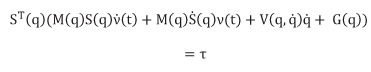
The two columns from S(q) are the null space from A(q) and are linearly independent. It presents q̇ as linear combination of two columns from S(q), q̇ = S(q)v Deriving q̇ we have q̇ = S(q)v̇(t)+Ṡ(q)v(t) and raplacing it in equation 14 gives as the result of equations 21 and 22:

$\begin{array}{c}\mathrm{M}\left(\mathrm{q}\right)=\left[\begin{array}{ccc}\mathrm{d}11& \dots & \mathrm{d}112\\ ⋮& \dots & ⋮\\ \mathrm{d}121& \dots & \mathrm{d}1212\end{array}\right]\ddot{\mathrm{q}}+\left[\begin{array}{c}\mathrm{h}1\\ ⋮\\ \mathrm{h}12\end{array}\right]\dot{\mathrm{q}}+\left[\begin{array}{c}\mathrm{c}1\\ ⋮\\ \mathrm{c}12\end{array}\right]=\left[\begin{array}{cc}0& 0\\ ⋮& ⋮\\ 1& 0\\ 0& 1\\ ⋮& ⋮\\ 0& 0\end{array}\right]\left[\begin{array}{c}{\mathrm{\tau }}_{\mathrm{x}}\\ ⋮\\ {\mathrm{\tau }}_4\end{array}\right]-\mathrm{ } \\ \left[\begin{array}{ccccccc}-{\mathrm{S}}_{\mathrm{C}}& {\mathrm{C}}_{\mathrm{C}}& 0& 0& 0& \dots & 0\\ {-\mathrm{C}}_{\mathrm{C}}& -{\mathrm{S}}_{\mathrm{C}}& -\mathrm{b}& \mathrm{r}& 0& \dots & 0\\ 0& 0& \mathrm{b}& 0& \mathrm{r}& \dots & 0\end{array}\right]\end{array}$

(18)

$\ddot{\mathrm{q}}={\mathrm{M}\left(\mathrm{q}\right)}^{-1}[\mathrm{E}\left(\mathrm{q}\right)\mathrm{\tau }-{\mathrm{A}}^{\mathrm{T}}\left(\mathrm{q}\right)\mathrm{\lambda }-\mathrm{V}\left(\mathrm{q},\mathrm{ }\dot{\mathrm{q}}\right)\dot{\mathrm{q}}-\mathrm{G}\left(\mathrm{q}\right)]$

(19)

$\mathrm{S}\left(\mathrm{q}\right)=\left[\begin{array}{ccccccc}-{\mathrm{S}}_{\mathrm{C}}& {\mathrm{C}}_{\mathrm{C}}& 0& 0& 0& \dots & 0\\ {-\mathrm{C}}_{\mathrm{C}}& -{\mathrm{S}}_{\mathrm{C}}& -\mathrm{b}& \mathrm{r}& 0& \dots & 0\\ 0& 0& \mathrm{b}& 0& \mathrm{r}& \dots & 0\end{array}\right]$

(20)

$\begin{array}{c}{\mathrm{S}}^{\mathrm{T}}\left(\mathrm{q}\right)\left(\mathrm{M}\left(\mathrm{q}\right)\mathrm{S}\left(\mathrm{q}\right)\dot{\mathrm{\nu }}\left(\mathrm{t}\right)+\mathrm{M}\left(\mathrm{q}\right)\dot{\mathrm{S}}\left(\mathrm{q}\right)\mathrm{\nu }\left(\mathrm{t}\right)+\mathrm{V}\left(\mathrm{q},\mathrm{ }\dot{\mathrm{q}}\right)\dot{\mathrm{q}}+\mathrm{ }\mathrm{G}\left(\mathrm{q}\right)\right)=\mathrm{ } \\ (\mathrm{E}\left(\mathrm{q}\right)\mathrm{\tau }-{\mathrm{A}}^{\mathrm{T}}\left(\mathrm{q}\right)\mathrm{\lambda }){\mathrm{S}}^{\mathrm{T}}\left(\mathrm{q}\right)\end{array}$

(21)

${\mathrm{S}}^{\mathrm{T}}\left(\mathrm{q}\right)(\mathrm{M}\left(\mathrm{q}\right)\mathrm{S}\left(\mathrm{q}\right)\dot{\mathrm{\nu }}\left(\mathrm{t}\right)+\mathrm{M}\left(\mathrm{q}\right)\dot{\mathrm{S}}\left(\mathrm{q}\right)\mathrm{\nu }(\mathrm{t})+\mathrm{V}\left(\mathrm{q},\mathrm{ }\dot{\mathrm{q}}\right)\dot{\mathrm{q}}+\mathrm{ }\mathrm{G}\left(\mathrm{q}\right))=\mathrm{\tau }$

(22)

Is verified that M(q) complies with n=m (square), M^T(q)= M(q) (symmetric). It is not singular (det (M(q)) = 8.0644e + 021 > 0 = det (M(q)^T) = 8.0644e + 021 > 0; d₁₁ = 0.219 > 0),) and therefore is inverse. M⁻¹(q) ∃M⁻¹(q) = (M⁻¹(q))⁻¹ > 0. It is also positive definite, in that M₁₁ (q) > 0 for all q and its determinant(M(q)) > 0.

3. Real experiment and positioning simulation

The real experiment and the simulation of positioning from the mobile manipulator is done according to the 5 real operation tasks. In order to realize these activities, the control strategy published by Yamamoto was used [29] in the paper dedicated to the control and coordination of movement from mobile manipulators in 2004. Using the vector in the state space x = [q^T v^T] ^T , we can represent the constraints and the motion's equations from the mobile manipulator in the state space:

$\dot{x}=\left[\begin{array}{c}Sv\\ f_2\end{array}\right]+\left[\begin{array}{c}0\\ {\left(S^{T}MS\right)}^{-1}\end{array}\right]\tau$

(23)

where f₂ = (S^TMS)⁻¹(-S^T MSv – S^TV). This equation is simplified in order to apply the following linear feedback: T̈ = S^T MS(u – f₂). Then, it could assume a new input u, which will linearize equation 23. Considering the linearization, it could be used in the desired trajectory y^d in order to feedback the error e = y^d – y:

$\ddot{y}=v={\ddot{y}}^d+K_d\left({\dot{y}}^d-\dot{y}\right)+K_d\left(y^d-y\right)$

(24)

From equation 24, v is obtained and then u and, therefore, ẋ. Finally, by integration, x can be obtained.

• a)

  Orientation (stage 2, task 1). The driving wheels are located on the left side at the front and right side rear, the alternate movement v_r = –v_r allows the rotation about axis z in the reference ratio of θ 1130 mm. This is using the transformation GT_C = A_C and q_M = [φ_C θ_rθ₁]^T. Therefore, it is assumed that the movement is in the horizontal plane [13], that the contact wheel is at one point, that the wheels are not deformable, that there is pure rotation at the contact point v = 0, that there is no slippage, and that the axis direction is orthogonal to the surface. The wheels are connected by a rigid body (chassis).

• b)

  Approximation / trajectories tracking (stage 4, task 2). The system executes the tracking of the desired trajectory, based in the transformation GT_C = A_C. The mobile platform is moved according to this equation, q_MR = [xyzφc θ_r θ₁]^T.

• c)

  Manipulation (stage 4, task 3). In the rank x=2. 5, y=2. 5 and z=1. 5 m, the kinematics is given by X_M =GT₄E E_μ by the equation q_M = [φ_c θ₁ d₂ θ₃ θ₄]^T.

• d)

  The lifting of the mobile manipulator in the rank from 0. 15 up to 0. 52 m based on the transformation GT_C = A_C, z is given by Z_C = var = λ_C0 + δλ_C, Z_C0 = λ_C0 = constant > 0, θ_C1 = variable, l_CS1 = constant > 0, φ = variable, where the increment δλ_C of z, depends upon the lifting arms.

• e)

  The lifting arms climb in the rank from 0. 15 up to 0. 47 m. The mobile manipulator with a mass m is moved on the sloped surface at an angle Ψ, with respect to the horizontal, given by the transformation CT_CS1, and the equation F_ascenso = mg(senΨ + μcosΨ), where g is gravity when θ_CS > 60°, λ_C + (δ_C = l_CS1 + sen θ_CS), in order to realize the climbing task. λ_C is variable and depends upon θ_CS.

4. Results

From the forward kinematics, the reference values for every task were taken. The parameters of the coordinate local “C” which is the base for obtaining the reference values are as follows: $\begin{array}{c}{\mathrm{A}}_{\mathrm{C}}:{\mathrm{x}}_{\mathrm{C}0}=2,\mathrm{ }{\mathrm{y}}_{\mathrm{C}0}=2,\mathrm{ }{\mathrm{z}}_{\mathrm{C}}={\mathrm{\lambda }}_{\mathrm{C}0}+{\mathrm{\lambda }}_{\mathrm{C}},\mathrm{ }{\mathrm{z}}_{\mathrm{C}0}={\mathrm{\lambda }}_{\mathrm{C}0}\\ =0.\mathrm{ }15,\mathrm{ }{\mathrm{\theta }}_{\mathrm{C}1}=\frac{\mathrm{\pi }}{2},\mathrm{ }{\mathrm{l}}_{\mathrm{C}\mathrm{S}1}=0.\mathrm{ }44,\mathrm{ }\mathrm{\phi }=\frac{\mathrm{\pi }}{4},\mathrm{ }\mathrm{\phi }=20\mathrm{\pi }\end{array}$ .

${\Delta \mathrm{\lambda }}_{\mathrm{C}}=\mathrm{v}\mathrm{a}\mathrm{r}\mathrm{i}\mathrm{a}\mathrm{b}\mathrm{l}\mathrm{e}=\left\{\begin{array}{c}{\mathrm{l}}_{\mathrm{C}\mathrm{S}1}{\mathrm{S}}_{\mathrm{C}1}-{\mathrm{\lambda }}_{\mathrm{C}0}+r\\ for {\mathrm{l}}_{\mathrm{C}\mathrm{S}1}{\mathrm{S}}_{\mathrm{C}1}-{\mathrm{\lambda }}_{\mathrm{C}0}+r\ge 0\\ 0 \text{for another case}\end{array}\right.,\mathrm{ }\mathrm{r}=0.\mathrm{ }08\mathrm{ }$

(25)

• a)

  Equation 26 is the transformation of the mobile platform rotating about its own axis:

  ${\mathrm{G}\mathrm{T}}_{\mathrm{C}}=\left[\begin{array}{cccc}1& 2.\mathrm{ }4493\mathrm{e}-015& 0& 0\\ -2.\mathrm{ }4493\mathrm{e}-015& 1& 0& 0\\ 0& 0& 1& 0.\mathrm{ }15\\ 0& 0& 0& 1\end{array}\right]\mathrm{ }$

  (26)

• b)

  Equation 27 is the transformation of the platform according to these parameters: ${{\mathrm{x}}_{\mathrm{C}}=2,\mathrm{ }{\mathrm{y}}_{\mathrm{C}}=2,\mathrm{ }{\mathrm{\lambda }}_{\mathrm{C}0}=0.\mathrm{ }15,\mathrm{ }\mathrm{\phi }}_{\mathrm{C}}=\frac{\mathrm{\pi }}{4},\mathrm{ }{\mathrm{\theta }}_{\mathrm{R}}=2\mathrm{\pi },\mathrm{ }{\mathrm{\theta }}_{\mathrm{L}}=-2\mathrm{\pi },\mathrm{ }\mathrm{b}=0.\mathrm{ }4,\mathrm{ }{\Delta \mathrm{\lambda }}_{\mathrm{C}}=0$ .

  ${\mathrm{G}\mathrm{T}}_{\mathrm{C}}={\mathrm{A}}_{\mathrm{C}}=\left[\begin{array}{cccc}0.\mathrm{ }7071& -0.\mathrm{ }7071& 0& 2\\ 0.\mathrm{ }7071& 0.\mathrm{ }7071& 0& 2\\ 0& 0& 1& 0.\mathrm{ }15\\ 0& 0& 0& 1\end{array}\right]$

  (27)

• c)

  Equation 28 is the transformation of the manipulator with the end effector: $\begin{array}{c}{{\mathrm{x}}_{\mathrm{C}}=2,\mathrm{ }{\mathrm{y}}_{\mathrm{C}}=2,\mathrm{ }{\mathrm{\lambda }}_{\mathrm{C}0}=0.\mathrm{ }15,\mathrm{ }\mathrm{\phi }}_{\mathrm{C}}=\frac{\mathrm{\pi }}{4},\mathrm{ }{{\mathrm{\lambda }}_0=0.\mathrm{ }16,\mathrm{ }{\mathrm{l}}_0=0.\mathrm{ }33,\mathrm{ }\mathrm{\theta }}_1=\frac{3\mathrm{\pi }}{4},\mathrm{ }{\mathrm{\lambda }}_2=1.\mathrm{ }4,\mathrm{ }{\mathrm{\theta }}_3=-\frac{\mathrm{\pi }}{2},\\ \mathrm{ }{{\mathrm{l}}_3=0.\mathrm{ }15,\mathrm{ }\mathrm{\theta }}_4=\frac{\mathrm{\pi }}{2},\mathrm{ }{\mathrm{\theta }}_{\mathrm{C}1}=\frac{\mathrm{\pi }}{2},\mathrm{ }{\mathrm{l}}_{\mathrm{C}\mathrm{S}1}=0.\mathrm{ }44,\mathrm{ }\mathrm{r}=0.\mathrm{ }08,\mathrm{ }{\mathrm{\lambda }}_5=0.\mathrm{ }38,\mathrm{ },\mathrm{ }{\mathrm{\lambda }}_6=0.\mathrm{ }25\end{array}$ :

  ${{\mathrm{X}}_{\mathrm{M}}-\mathrm{G}\mathrm{T}}_4\mathrm{E}{\mathrm{ }\mathrm{E}}_{\mathrm{\mu }}=\left[\begin{array}{cccc}\mathrm{ } 0.\mathrm{ }7071\mathrm{ } & 0.\mathrm{ }5000& 0.\mathrm{ }5000& 2.\mathrm{ }8567\\ \mathrm{ }-0.\mathrm{ }7071& 0.\mathrm{ }5000& 0.\mathrm{ }5000& 2.\mathrm{ }8567\\ \mathrm{ }0& -0.\mathrm{ }7071& 0.\mathrm{ }7071& 1.\mathrm{ }3305\\ 0& 0& 0& 1\end{array}\right]\mathrm{ }$

  (28)

• d)

  Equation 29 is the transformation at the time that the platform is lifting: 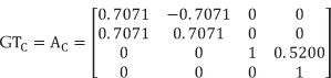${\mathrm{x}}_{\mathrm{C}}=0,\mathrm{ }{\mathrm{y}}_{\mathrm{C}}=0,\mathrm{ }{\mathrm{\theta }}_{\mathrm{C}1}=\frac{\mathrm{\pi }}{2}:$ :

  ${\mathrm{G}\mathrm{T}}_{\mathrm{C}}={\mathrm{A}}_{\mathrm{C}}=\left[\begin{array}{cccc}0.\mathrm{ }7071& -0.\mathrm{ }7071& 0& 0\\ 0.\mathrm{ }7071& 0.\mathrm{ }7071& 0& 0\\ 0& 0& 1& 0.\mathrm{ }5200\\ 0& 0& 0& 1\end{array}\right]$

  (29)

• e)

  Equation 30 is the transformation corresponding to climbing: ${{\mathrm{x}}_{\mathrm{C}}=0,\mathrm{ }{\mathrm{y}}_{\mathrm{C}}=0,\mathrm{ }{\mathrm{\lambda }}_{\mathrm{C}0}=0.\mathrm{ }15,\mathrm{ }\mathrm{\phi }}_{\mathrm{C}}=\frac{\mathrm{\pi }}{4},\mathrm{ }{\mathrm{\theta }}_{\mathrm{C}1}=\frac{\mathrm{\pi }}{2},\mathrm{ }{\mathrm{\theta }}_{\mathrm{C}\mathrm{S}1}=-\frac{\mathrm{\pi }}{2},\mathrm{ }\mathrm{d}=0.\mathrm{ }35,\mathrm{ }{\mathrm{l}}_{\mathrm{C}\mathrm{S}}=0.\mathrm{ }33,\mathrm{ }{\mathrm{l}}_{\mathrm{C}\mathrm{S}1}=0.\mathrm{ }44,\mathrm{ }\mathrm{r}=0.\mathrm{ }10$ .

  ${\mathrm{G}\mathrm{T}}_{\mathrm{C}\mathrm{S}1}=\left[\begin{array}{cccc}0.\mathrm{ }7071& 0& -0.\mathrm{ }7071& 0\\ 0.\mathrm{ }7071\mathrm{ }& 0& 0.\mathrm{ }7071\mathrm{ }& 0\\ 0& -1& 0& 0.\mathrm{ }47\\ 0& 0& 0& 1\end{array}\right]$

  (30)

Taking the reference values, several simulations using equation 30 for the real operational scenarios were carried out, where the errors and performance index were obtained, as shown in tables 2 and 3.

Table 3.

Tasks for manipulation, lifting and climbing

In Table 4, the results of real experiments in the mobile manipulator are shown, focusing on the maximum and minimum errors according to the reference values.

Table 4.

Real experiments for the manipulation, lifting and climbing tasks.

30 samples	Deviations
1. In the test for orientation the next errors were taken:	Error min. 40 mm	Error max. 80 mm.
2. Approaching (trajectories tracking).	Error min. 0. 5 mm	Error max. 8 mm.
1. Manipulation (positioning).	Error min. 0. 5 mm	Error max. 8 mm.
2. Lifting.	Error min. 4 mm	Error max. 6 mm.
3. Climbing.	Error min. 4. 6 mm	Error max. 8 mm.

In Figure 6, we see the mobile manipulator in a real experiment approaching and positioning the end effector in the target.

5. Discussion

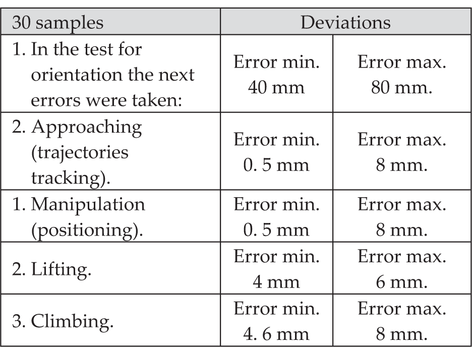
The real experiment was carried out on the floor inside a laboratory, which helped in the measurement of the registered parameters; however, measurements in rough ground were not taken due to a lack of adequate methods and instrumentation for the corresponding measurements of its parameters. The comparison of the errors of the simulations and the real experiments of the 5 evaluated tasks are presented in Table 5. As many as 30 samples were taken for each task, which validates the kinematic modelling.

Table 5.

Simulation and real experiments for the tasks.

Task	Performance [mm]
	Simulation (ē y RMS)		Real system (ē y RMS)
Orientation.	40 and 40. 161		60 and 60. 0922
	Error due to the wheel slipping on the floor.
Approaching.	2. 37 and 2. 376		6. 5 and 6. 5236
	The 2 tests were performed at 0. 5 m /s.
Manipulation.	0. 050 and 0. 051		4. 25 mm and 4. 25002
	This is due to slip of wheels on the floor.
Lifting.	0. 020 and 0.02144		5 and 5. 037658
	Due to adjustment and weight of system.
Climbing.	0. 040 and 0.040743		6. 3 and 6. 30918
	This is due to the deformation of the rear wheels and its adjustment, in addition to its weight.
	8. 497	8. 5299	16. 41	16. 447
	With load		Without load
Dynamic analysis with software CAE	The mass centre varies in φ 60.		The mass centre varies in φ 40.
	The greatest variation occurs in Z.
	The stress due to a load of 14 kpa.		The stress due to a load of 7 kpa.
	The deformation of λ2 is 1. 055.		The deformation of λ2 is 0. 03.
	It was validated to the fullest extension and in the normal state of the prismatic joint.

According to the manual of explosives, deactivation [24] must be considered with a maxim um handling error of 10 mm.

In Table 6 is shown the differences in errors between the simulation and the real experiments of the 5 evaluated tasks. The figures are described in the Gaussian bell form, with the results of the simulation in blue and the experiment in red, including the mean and the R. M. S error.

Table 6.

Errors between the simulation and the real experiment.

Comparison of the simulation and the real experiment
Tasks			Difference
1. Orientation.			ē	20 mm
			RMS	19. 94 mm
2. Approaching.			ē	4. 12 mm
			RMS	4. 147 mm
3. Handling.			ē	4. 2 mm
			RMS	4. 19 mm
4. Lifting.			ē	4. 98 mm
			RMS	5. 01 mm
5. Climbing.	ē	6. 26 mm
	RMS	6. 28 mm

The orientation error is very large due to wheel slippage on the ground, as well as the tracking of the trajectory where the trajectory is a point referenced by the mass centre of the mobile manipulator; the aforementioned variations are due to the compensation of the control of the non-holonomy of the system caused by the non-integrable solutions of the wheels.

Figure 7.

Error simulation against the error of the real experiment for the manipulation task

6. Conclusion

A methodology for the positioning of the multi-articulated mobile manipulator by means of the development of a kinematical model is defined, explained and assessed, where the use of a novel scheme to devise the homogeneous transformations achieves the given structure for the forward kinematics. The methodology has the following advantages: (1) it provides a big picture for mechatronic design when it develops the modelling and simulation of the mobile manipulator; (2) it simplifies the estimation of the homogenous transformation when it is required; (3) it allows the determination of the parameters of interaction when it is necessary to make the schemes in a coupled way; (4) it is easy for kinematic modelling when any added subsystem is incorporated in the analysis of the performance index based on the error of the real operational scenarios:

The simulations have an average error RMS of 3. 47 mm with regard to the references values, while the real experimentations have an error RMS of 7. 91 mm. These are permissible errors in relation to the error of 10 mm, which is specified in the tasks for the deactivation of explosives [30]. The maxim deformation of the manipulator with a load of 10 kg was 1 mm.

The major advantages of this proposal in comparison with previous work are considered, such as the contributions of this paper: the development of kinematic modelling in a coupled way for a wheeled mobile manipulator with 12-DOF, the extension of homogeneous transformation graphs which organize in a modular way the transformations of every link so as to obtain the kinematics of the mobile manipulators and the proposed methodology formodelling the positioning in real operational scenarios.

As to future work, by means of a visual feedback system, will be determined the position of the explosive device incorporating a vision system to detect the coordinates of targets, placing some sensors at the end effector for use in different kinds of manipulation based in the device's form, and finally implementing the proposed modelling methodology in the design of mobile systems with different manipulators.

Footnotes

7. Acknowledgements

The authors would like to acknowledge the Centro de Ingeniería y Desarrollo Industrial (CIDESI) [] for funding this work.