Sage Journals: Discover world-class research

Abstract

In this paper, we propose an online key object discovery and tracking system based on visual saliency. We formulate the problem as a temporally consistent binary labelling task on a conditional random field and solve it by using a particle filter. We also propose a context-aware saliency measurement, which can be used to improve the accuracy of any static or dynamic saliency maps. Our refined saliency maps provide clearer indications as to where the key object lies. Based on good saliency cues, we can further segment the key object inside the resulting bounding box, considering the spatial and temporal context. We tested our system extensively on different video clips. The results show that our method has significantly improved the saliency maps and tracks the key object accurately.

Keywords

Saliency Context Key Object Tracking Extraction

1. Introduction

Object detection and tracking are essential technologies used in computer vision systems to actively sense the environment. Since the Internet and digital recording techniques are developing quickly, the number of videos to investigate has become huge. In fields such as video surveillance [1], video compression [2] and video summarization [3], people need to capture all kinds of interesting information from videos. Meanwhile, with the development of robotic and unmanned technologies, automatically detecting and tracking interesting objects with little prior knowledge has also become more and more important. We call these interesting objects the key objects.

According to information theory, a key object carrying lots of information should have significant difference to the background scene. This also indicates that the key object is unpredictable and the initial state of the tracker is not likely to be manually provided. To solve this problem, many bottom-up saliency detection methods driven by low level features are proposed. These techniques have already been widely used on static image analysis [4–5]. In recent years, some literature has extended saliency features to the temporal domain [6–7]. Also, some methods have been proposed to detect and track key objects in video clips with bottom-up saliency.

There are two main problems with detection and tracking key objects with saliency features. The first one is the inaccuracy of the saliency maps. Most of the saliency computation methods only provide a fuzzy indication of the foreground and background objects. The saliency maps are blurred around the key object area, which will make the tracking inaccurate. Moreover, it is very hard to extract the exact key object boundary from such saliency maps. Another problem of using saliency features is that in different frames or between different scenes, neither the static nor the motion cues may be reliable. For example, a person in green clothes walking on grass is hard to capture with static saliency, but can easily be found in the motion field. On the contrary, when the object stops, we need to use a colour or texture cue to facilitate the motion tracker, otherwise it will fail easily.

In this paper, we introduce a saliency refinement scheme based on the spectral affinity from colour and motion features. This mechanism injects the spatial context information into saliency maps to raise the compactness of the saliency inside the key object. The raw input saliency features are computed following the work of Liu in [4] and [6]. When computing the motion saliency, we use the popular variational optical flow [8], which is accurate and has been implemented on GPU to achieve real-time performance. Our context-aware saliency maps help our tracking system to achieve more accurate tracking results than by directly using the fuzzy saliency maps produced by Liu's method. Our saliency maps are also better for the further segmentation task.

During tracking, we introduce an adaptive weight tuning scheme to integrate static and dynamic saliency features to discover and track the key object [9]. This scheme is based on the compactness of saliency maps. It sets a higher weight to the map that has more compact high values in the key object area. The tracking problem is formulated in a CRF-filtering framework in which the key object is represented as a bounding box to reduce the searching dimension. We employ a Particle Filter (PF) to solve this inference problem. The initialization of PF is achieved using a Monte Carlo sampling method.

Any approach that attempts to extract the object from the video clip would ideally result in pixel-wise segmentation. The tracked bounding boxes provide us with clear background indication so that we can model the features of the surrounding area as background. Then it is much easier and more efficient to extract the key object boundary inside the bounding box. To take temporal context into consideration, we perform a 3D graph-cut on the super-pixels to get the accurate key object segmentation. The super-pixels are computed based on the Gabriel graph [10], which is a subset of the constrained Delaunay triangulation [11].

The main contributions of this paper can be summarized as follows. First, we propose a context-aware saliency computation mechanism, which can refine any saliency map to produce more accurate key object indication.

Second, we propose an adaptive weight tuning scheme to fuse the static and dynamic saliency map. Third, we provide a triangulation based on a super-pixel generation method and perform it inside the bounding box to segment the key object accurately and efficiently. Fourth, we have built a salient object tracking database (AIAR-SoT), which contains 26 video clips of about 2500 frames. All the salient objects in all the frames are labelled.

2. Related Work

Long-duration tracking is always a challenging problem for computer vision, because the targets may undergo large uncertainties in their visual appearance and the real environments can be cluttered and distractive. In order to overcome these difficulties, a variety of tracking algorithms are proposed and implemented. For example, Condensation [12], Mean-Shift [13] and probabilistic data association filters [14].

Generally, a tracking algorithm has two major components: the algorithm framework and the representation model of the object. There have been many effective tracking frameworks, including deterministic methods used in [15] and stochastic methods such as the Particle Filter [16] and Kalman Filter (KF) [17].

The representation model is a consistent description of the object, which is essential for reliable tracking and has been studied by researchers for a long time. Colour [12, 15, 18] and geometry information [19] are most widely used as the appearance models. Among them, the colour histogram feature proposed in [18] is always popular due to its efficiency. However, early tracking approaches assume that the appearance of the target stays consistent and use the target's model in the first frame as a global tracking template. However, for real tracking problems, the appearance of the target always changes obviously due to its motion, environment illumination and camera movement, which makes the naive approaches less likely to achieve good results over a long duration.

To solve this problem, many researchers use adaptive models, which change with respect to the observation [20–21]. For example, [20] presents an adaptive probabilistic tracking algorithm that updates the models using an incremental update of eigenbasis. One drawback of these methods is the model drifting problem, which is caused by considering occlusion or background as a part of the target during updating. To avoid drifting, the author of [21] introduces a small threshold, which enforces the requirement that the result of the second gradient descent should not diverge too far from the result of the first.

In fact, tracking is a binary annotation problem of object and background. Therefore, Avidan proposed several classifier-based tracking approaches, e.g., SVM tracking [22] and Adaboost tracking [23]. These approaches take the difference between object and environment into consideration and have good adaptability. But these approaches need off-line training. Therefore, they can only track certain kinds of objects.

As indicated in the classifier-based approaches, the divergence between object and background is an important cue. In [24], the author declares that the features that best discriminate between object and background are also best for tracking the object. The author of [25] uses the idea of saliency when he extracts stable patches with a gradient descent algorithm as the object model.

Visual saliency is computed from two classes of visual stimuli: a class of stimuli of interest and a background [5]. It is invariant to the changing of object appearance and can be used for the automatic initialization of the tracker. [5] proposes a biologically inspired tracking framework based on discriminate centre-surround saliency. The author of [26] extracts the salient region using an oriented Gabor filter and K-means, and then tracks the region for a short period of time. The author of [27] proposes a context-aware saliency computation method, which aims to detect the image regions that represent the scene. It is only recently that literature has begun to focus on saliency based on motion information. In [6] Liu combines static and dynamic saliency features in Dynamic Conditional Random Field (DCRF) [28], under the constraints of a global topic model. This approach achieves good results on many challenging videos, but it needs the whole video series to compute the global topic model, which makes it only an off-line method. Recently, the author of [7] proposed a spatial-temporal saliency algorithm based on a centre-surround framework. They use a fix-size window to extract centre-surround saliency to track objects. However, this can only track objects of relatively small sizes.

3. Proposed Method

We propose an on-line system that detects and tracks the key object, which has high visual saliency in a video clip. We use a Particle Filter to track the key object and use 3D-GraphCut on super-pixels to extract the object boundary. The basic pipeline of our system is shown in Figure 1.

Figure 1.

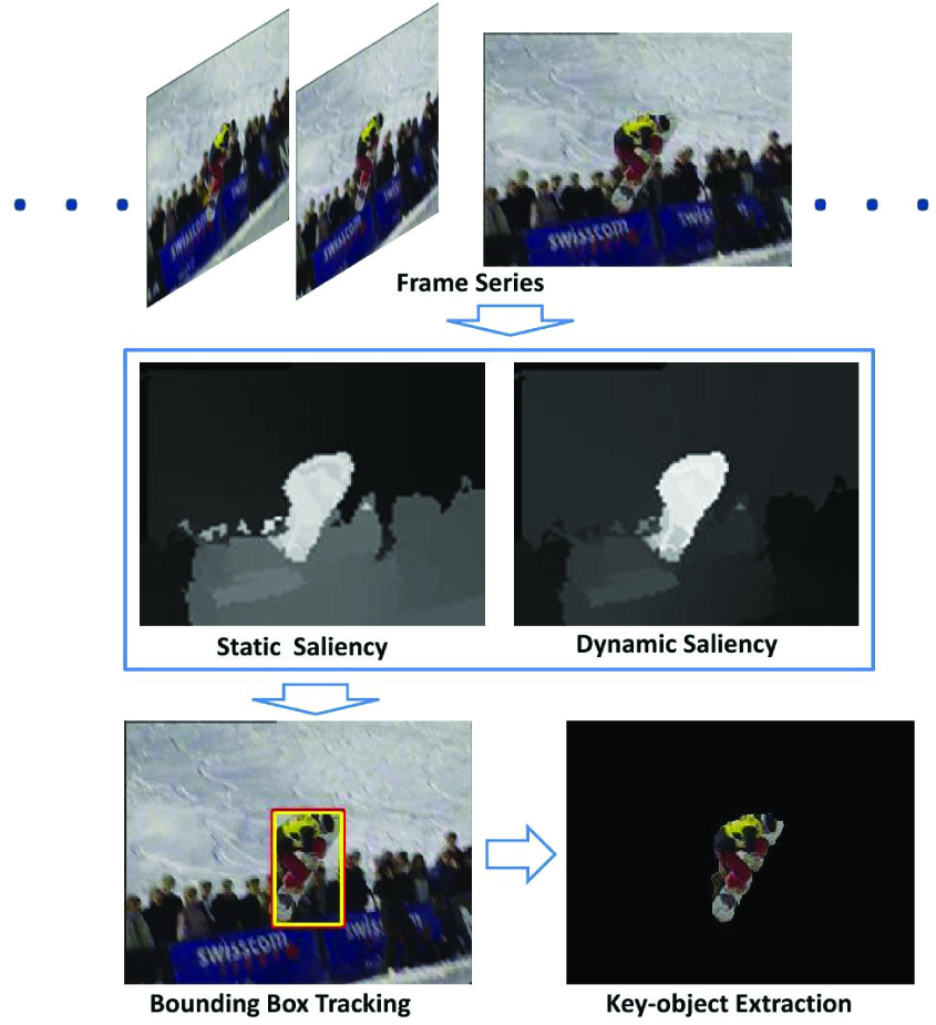
The system pipeline

3.1 Context-Aware Saliency

The saliency maps generated by most of the methods in the literature are so fuzzy that the boundaries of the object are blurred and some noisy spots may appear. The main reason for this is because the saliency operators, such as the boundary detector or centre-surround filter, are relatively local, so it is hard to adapt these operators without knowing the scale of the saliency object.

We propose a context-aware computation method to improve the saliency maps. To get the raw input saliency maps, we follow Liu's work both on colour images [4] and on motion fields [29]. The motion field we use is computed by the popular variational optical flow algorithm [8].

To refine the saliency maps considering the whole image, we aim to find a function, which computes the saliency value of each pixel considering the saliency of other pixels. The function sets high weights on the pixel's nearest neighbours and sets lower or zero weights to other pixels. Therefore, this non-parametric function can be seen as an affinity matrix that indicates the likelihood of neighbouring in the feature space. The affinity can be measured by low-level cues such as colour, texture and motion. However, affinity computation is only reliable inside a small neighbourhood of the pixel. The affinity value computed from two pixels far away tends to be highly noisy.

To solve this problem, we introduce spectral affinity into saliency computation to refine the saliency maps. Every pixel adaptively gathers information from its spectral embedding neighbourhood. The refinement contains the following steps.

First, we set a locally connected graph, whose nodes are pixels and edges are affinities, computed from colour and motion cues.

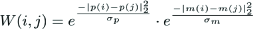
W (i, j) = e^{\frac{- | p (i) - p (j) |_{2}^{2}}{σ_{p}}} \cdot e^{\frac{- | m (i) - m (j) |_{2}^{2}}{σ_{m}}}

(1)

where |p(i)–p(i)|2 < r, i and j are two pixels within a specific distance, r = 10. p(·) represents spatial location and m(·) is a feature vector containing colour and motion information. The weight W(i,j) = 0 is for any pair of nodes that are more than ^r pixels apart.

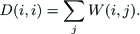
Second, we obtain spectral embedding by solving the generalized eigenvector problem(W, D), where D stands for the diagonal degree matrix.

D (i, i) = \sum_{j} W (i, j) .

(2)

This is equal to solving the eigenvector problem of the normalized affinity matrix $D^{- \frac{1}{2}} W D^{- \frac{1}{2}}$ .

Third, having the eigenvectors V corresponding to the k largest eigenvaluesA, we consider the low-rand approximation of the normalized affinity matrix.

\hat{W} = V \cdot Λ \cdot V^{T} .

(3)

The reconstructed matrix is more compact than W and is fully connected. The eigenvalues of the normalized affinity matrix range from 0 to 1. Therefore, we adaptively choose k such that we only keep the eigenvalues higher than 0.98. This embedded affinity matrix assigns the neighbourhood of every pixel softly (in contrast to super-pixel based neighbourhood).

Finally, we re-compute the saliency value of each pixel as a weighted summation.

\hat{F} (i) = \sum_{j} \hat{W} (i, j) \cdot F (j),

(4)

where F(·) is the value of the raw saliency map and F̂(·) is the refined value. Ŵ is normalized row-wise to guarantee convex combination. Figure 2 demonstrates this refining procedure.

Figure 2.

Demonstration of our saliency computation. Saliency information is re-organized based on the spectral embedding. The left two maps show spectral affinity of the points marked as stars. Warmer colour indicates higher affinity. (figure best seen in colour)

3.2 Key object Tracking

Our key object discovery and tracking problem is formulated as a binary labelling task on a visual saliency map. We solve it sequentially using a particle filtering technique [16]. When initializing the tracker, we sample particles from the proposal distribution, which is determined by the saliency maps of the first two frames. New particles in the updating stage of PF are generated from the state transition model and are evaluated with both the saliency feature and the boundary closeness in the new frame. Figure 3 demonstrates this procedure.

Figure 3.

The demonstration of the our tracking procedure.

3.2.1 Particle Filter

For a given image series I_1:t, particle filter is an inference technique to estimate the unknown motion state X_t from the observations, Y_1:t, where X is the binary labelling of the key object. However, directly inferring an object's boundary is a high-dimensional task and is very inefficient to solve, so in the tracking stage we simplify the target model to a rectangular bounding box. By doing this, the state of object becomes the position and size of the object, X_t = (x_t,y_t,w_t,h_t), X_t ε ℝ⁴.

The particle filter approximates the posterior distribution by a set of weighted particles ${X_{t}^{(j)}, w_{t}^{(j)}}_{j = 1}^{J}$ . The Maximum A Posterior (MAP) estimate is usually used to get the state estimation.

{\hat{X}}_{t} = a r g \max_{X_{t}} P (X_{t} | Y_{1 : t}) \approx a r g \max_{X_{t}} w_{t}^{(j)},

(5)

where w^(j)_t is the weight at frame t for particlej.

We apply the direct version of Monte Carlo importance sampling technology [30] in the update stage to avoid degeneracy. It contains the following steps.

First, we draw J samples x^(j)_t from the proposal distributionQ(X_t):

x_{t}^{(j)} ~ Q (X_{t}) = \sum_{j} w_{t - 1}^{(j)} P (X_{t} | X_{t - 1}^{(j)}) .

(6)

where w^(j)_t-1 is the weight of the j – th particle in the previous frame. We use a typical linear Gaussian transition model to sample the current particles from the important particle of the previous frame.

Second, the weight w^(j)_t is computed as the likelihood.

{\tilde{w}}_{t}^{(j)} = P (Y_{t} | X_{t}^{(j)}) .

(7)

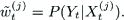
This re-weighting takes the observation evidence Y_t in to consideration. We normalize the weight.

w_{t}^{(j)} = \frac{{\tilde{w}}_{t}^{(j)}}{\sum_{k} {\tilde{w}}_{t}^{(k)}} .

(8)

3.2.2 Observation Model

A straightforward way to compute the likelihood is from the saliency map. Moreover, to make the tracking accurate, we hope our bounding box is as close to the object boundary as possible. Therefore, we use both saliency and edge cues to compute the weight.

{\tilde{w}}_{t}^{(j)} = e^{- D_{t}^{(j)} ∕ σ_{D}} \cdot e^{- F_{t}^{(j)} ∕ σ_{F}},

(9)

where σ_F and σ_D are the empirical parameters. D^(j)_t is the boundary closeness of X^(j)_t which is defined as the mean of four the minimum distance from the box boundary to the image edge. This can be easily computed from the distance transformation of any kind of edge map. F^(j)_t is the mean of saliency inside X^(j)_t, integrating the static and dynamic saliency features as a convex combination.

F_{t} = α_{s} F_{s, t} + α_{m} F_{m, t},

(10)

where F_s,t and F_m,t are the static and dynamic saliency maps respectively. ‘

We propose a spatial variance based method to compute the coefficients α_s and α_m. It is clear that in an informative saliency map, salient pixels should be spatially compact. We measure the map's compactness using the spatial variance var of the high values, which are approximately determined with Otsu's threshold [31]. For example, in the static map.

v a r_{s} = \sqrt{\frac{1}{| ℙ |} \sum_{p \in ℙ} | p - \bar{p} |^{2}}, ℙ : {p | F_{s} (p) > t h r_{s}},

(11)

where ℙ is the set of the coordinates of the high values and |ℙ| its size, thr_s is Otsu's threshold and P̄ is the mean of P̄. For the dynamic map, var_m is computed similarly.

The weights of the saliency maps are computed inversely proportional to their spatial covariance.

α_{s} = \frac{v a r_{m}}{v a r_{s} + v a r_{m}}, α_{m} = \frac{v a r_{s}}{v a r_{s} + v a r_{m}}

(12)

3.2.3 Initialization

Different from many tracking approaches, which need a pre-determined object prior, our approach automatically discovers the salient object to initialize the tracker. We use the fused saliency map from the first two frames as the proposal distribution to estimate X₀.

First, we draw samples from the proposal distribution Q(X_o). Let {(X₀^(j), w₀^(j) denote the particles generated by the samples and their weights. The weights are computed the same way as in the updating stage of the particle filter and the estimation of X₀ is defined as:

{\hat{X}}_{0} = a r g \max_{X_{0}^{(j)}} X_{0}^{(j)} \cdot w_{0}^{(j)} .

(13)

Thanks to our more discriminative saliency map, this estimation is accurate enough to initialize the particle filter.

3.3 Key object Segmentation

Any approach that attempts to extract an object from a video clip would ideally result in pixel-wise segmentation instead of bounding boxes. An accurate segmentation is helpful for lots of further procedures such as action recognition and object matching. In this paper, we propose the segmentation as a procedure based on the sequential tracking result. There are two main advantages of doing so. First, segmenting inside the bounding box is more reliable and more efficient than doing it on the whole picture. Second, the bounding box provides us with reliable evidence of the background area, which can be modelled, based on the area surrounding the bounding box.

To extract the key object boundary in I_t, we perform a super-pixel based 3D-GraphCut on recent saliency maps ${F_{t - l}, \dots, F_{t - 1}, F_{t}}$ is used in our implementation. This algorithm also takes temporal context into consideration and is more robust than simply doing GraphCut on a single frame. We set up our graph as G = {V, E_s, E_t}. The nodes V are super-pixels and two kinds of edges are contained, where E_s contains edges between nodes in the same frame and E_t contains edges that link the nodes in consecutive frames.

We use a Gabriel graph [10] based on super-pixel representation. A Gabriel graph is a subset of a Delaunay triangulation. It contains only the Delaunay edges that serve as diameters of circles not enclosing any other points. The Delaunay graph is generated using constrained Delaunay triangulation [11], which doesn't create any Delaunay edges across the linked edge fragments on edge map. Constrained triangulation bridges gaps between edge fragments, while preserving the topology of the image. Another reason why we use the Gabriel graph is that it produces much bigger super-pixels than triangulation. To avoid deleting the gap-bridging edges, we force the Gabriel graph to keep the Delaunay edges, which are near the high gradient area of the motion field. We show the constrained Delaunay triangulation and the corresponding Gabriel graph in Figure 4.

Figure 4.

(a) shows the constrained Delaunay Triangulation. (b) shows the Gabriel Graph. In both graphs, the blue lines stand for the Delaunay edges while other coloured lines are detected edge fragments. (Figure best seen in colour)

The data cost V(s) of a super-pixel is set according toFS.

\begin{array}{l} V (s, b) = m i n (\sum_{p \in s} F S (p), 0.1 \cdot | X |) \\ V (s, f) = m i n (\sum_{p \in s} (1 - F S (p)), 0.1 \cdot | X |), \end{array}

(14)

where V(s,b) and V(s,f) are the cost of setting super-pixel s to the background and key object respectively. |X| is the area of the bounding box. Note that we take the summation instead of the mean with respect to the size of the super-pixel, because sometimes background may be set as a single super-pixel. Putting an upper bound on the cost helps maintain graph balance.

Pair-wise smooth E_s inside the frame is defined on the gradient value of the boundary. The GraphCut is likely to smooth over when E_s is high. We decrease E_s on the Delaunay edges because we want to close the region while the gradient information is weak there.

E_{s} (e) = {\begin{cases} \frac{1}{| e |} \sum_{p \in e} 1 - P b (I_{t}), i f e \notin D E \\ \frac{1}{2 | e |} \sum_{p \in e} 1 - P b (I_{t}), i f e \in D E, \end{cases}

(15)

where Pb represents the Probability of Boundary [32]. Dε is the set of Delaunay edges kept in the Gabriel graph.

Cross-frame pair-wise smooth E_t is defined based on the optical flow. GraphCut tends to put the same label on two super-pixels where E_t is high. Assume S₁, and S₂, are two super-pixels on I_t-1, and I_t respectively. We define the pair-wise smooth as the portion of the number of shared points to the minimum size of the two super-pixels.

E_{t} (s_{1}, s_{2}) = \frac{| ({\tilde{s}}_{1} \cap s_{2}) |}{\min (| {\tilde{s}}_{1} |, | s_{2} |)},

(16)

where s˜₁ is warped from s₁, using optical flow. |·| computes the area.

4. Experiments

In this section, we run our approach on various video clips with different topics. To demonstrate the performance of the saliency features, we evaluate our context-aware saliency maps compared to the input saliency maps and the approach of [27]. We also show the tracking results using static and dynamic features and compare the results of our approach with those of MeanShift [15] and the saliency tracker [4] on videos with challenging environment conditions. Finally, we show our key object segmentation results and compare with two baseline approaches.

4.1 Key object Segmentation

We have built a Salient object Tracking (AIAR-SoT) database with videos containing unambiguous topics. This database contains 31 videos of about 3000 frames and we are still enlarging it. These videos are either collected from video sharing web sites or recorded around our campus by a hand held video camera. The categories of the objects are various, containing people, vehicles and animals. The bounding boxes of the salient objects in all the frames are carefully labelled. To evaluate the performance of our saliency map and segmentation, we further labelled a subset of the database with exact segmentation masks. Some screen shots of the video clips are shown in Figure 5. This dataset can be downloaded from our website:

http://www.aiar.xjtu.edu.cn/personal_web/teacher&doctor/gzhang/file/AIAR-SoT.zip

Figure 5.

Our Salient object tracking database (AIAR-SoT). (a) shows some screen shots from the video clips overlapped with the labelled bounding box. (b) shows the corresponding segmentation ground truth.

4.2 Evaluation Criteria

To evaluate the discriminatively of our saliency map, we set up a criteria based on the segmentation ground truth.

For key object detection and segmentation task, we hope the saliency map will have high values inside the object area and low values outside. So we set up a criterion Δ_fb as follows.

\begin{array}{l} μ_{f g} = \sum_{L (p) = 1} F (p) ∕ \sum_{L (p) = 1} 1 \\ μ_{b g} = \sum_{L (p) = 0} F (p) ∕ \sum_{L (p) = 0} 1 \\ Δ_{f b} = μ_{f g} - μ_{b g}, \end{array}

(17)

where L is the segmentation ground truth (0 for background and 1 for object). Δ_fb reflects the difference of the mean values inside and outside the object area. A good saliency map should have high A_fb. Note that this criterion is only computed inside the 20% expanded ground truth bounding box because the points far away from the object don't confuse the computation.

With the labelled bounding box X_G and the tracked bounding box X, we use precision, recall and F-measure as the region-based measurements. F-measure is the harmonic mean of precision and recall. Precision is the fraction of the correctly detected region to the detected region while recall is that to the ground truth salient region. High precision can be achieved when the detected area is so small that it is totally inside the salient object. Similarly, high recall can also be achieved when the detected area is so big that both the salient object and the background are all contained in it. So, F-measure is defined to bear both high precision as well as high recall.

F_{α} = \frac{(1 + α) \cdot p r e c i s i o n \cdot r e c a l l}{α \cdot p r e c i s i o n + r e c a l l}

(18)

where α is the harmonic coefficient and is set to 0.5 following [32]. It is obvious that the F-measure will reach its peak of 1 when the detected area and the hand-annotated area are identical.

We use the boundary displacement error (BDE) [33], which measures the average displacement error of the corresponding boundaries, as the boundary based criterion. For the rectangular model, the definition of BDE is simplified as:

B D E = ‖ X - X_{G} ‖_{2}

(19)

which is the L2-norm of the position and size differences. A lower BDE indicates better boundary fitting.

To evaluate our object extraction approach we adapt the F-measure criteria, where the precision and recall are computed, by comparing our segmentation with the ground truth mask.

4.3 Context-Aware Saliency

We compare our refined saliency maps with the input saliency map [4] using the Δ_fb criteria. In Figure 6, we show some cases when the baseline saliency maps are not very discriminative, while our approach collects the saliency information from the spectral neighbour of each pixel and makes the saliency information more compact. We also compare our static saliency maps with a state-of-the-art context-aware static saliency computation method [27]. From the figure we can see [27]'s approach doesn't give a clear indication of the salient object area. It tries to fire the salient boundaries. Also, the results show that on some background points, values of our saliency maps are increased because of a smoothing effect. However, this is not a problem for further tracker or segmentation tasks because all the points inside the key object have higher saliency values than those on the background, so the boundaries of the key object become clearer.

Figure 6.

Comparison between the original saliency maps and our context-aware saliency maps of the frames shown in Fig. 5. (a) and (b) are the original static and dynamic saliency maps. (c) and (d) are the context-aware static and dynamic maps. (e) shows the saliency maps generated by the method of [27]

Table 1 shows the statistical comparison. To be fair, all the saliency maps are normalized to [0, 1]. It is clear that our method makes a significantly improvement to the input map and also outperforms [27]'s method.

Table 1.

Saliency map evaluation comparison

	Δ_fb,s	Δ_fb,m
Goferman's method [27]	0.237	–
Liu's method [4]	0.158	0.105
Our approach	0.259	0.236

The dynamic maps are improved much more than the static maps. This is because optical flow always smoothes over the object boundary, which makes the dynamic saliency map have high values outside the boundary. However, our context-aware saliency suppresses these false high values because their spectral neighbours are background.

4.4 Saliency Feature Integration

As discussed before, static and dynamical saliency features play important roles in different situations. To demonstrate the effectiveness of our feature integration, we run our approach on the AIAR-SoT database using 3 kinds of combinations of static and dynamic saliency maps as follows.

C1: The static saliency map

C2: The dynamic saliency map

C3: The adaptive combination of the two saliency maps

Figure 7. shows the precision, recall, F-measure and BDE of the three approaches. The static features and dynamic features are distinctive in different situations, so the F-measure of approach C1 and C2 are similar. Approach C3, combining both kinds of saliency features, improves F-measure by 16.7% compared with approach C1. C3 also improves F-measure by 15.9% compared with C2. The BDE evaluation of C3 is smaller than those of C1 and C2, implying that the results of C3 fit the boundary of the saliency objects better.

Figure 7.

Evaluation of saliency features for tracking. In (a) and (b) 1-3 corresponds to approach C1-C3 respectively.

To demonstrate the adaptive feature combination scheme, we show an example from experiment C3.

Figure 8 shows the static and dynamic saliency maps and the tracking results of C3. It also shows the change of combination weights due to the reliability of the static and dynamic saliency maps. In frame #1, the background is highly un-textured, which causes the variational optical flow to smooth over the object boundaries a lot. therefore, the dynamic map is not very discriminative and the weight becomes much lower. Around frame #15, the player is overlapped with the crowd and is not easily verified by colour. During this time, dynamic feature dominates the integration. When the player is in the sky, around frame #38, both maps are very discriminative so they have similar weights. Finally, in the last part of the clip, around frame #64, the camera movement is not stable because it is trying to follow the fast moving player. The aliasing effect becomes very strong, which blurs the object boundaries and also affects the optical flow computation. Therefore, neither of the static or dynamic maps is robust during this period, so the weights change a lot in the last part of the video.

Figure 8.

Results of the 'SnowBoard3’ clip with approach C3. (a) shows frame #1, #15, #38, #64 overlapped with the tracking results. (b) shows the colour coded optical flow. (c) are the corresponding static saliency maps. (d) are the corresponding dynamic saliency maps. (e) the curves show the change of weights in different frames.

4.5 Salient object tracking comparison

In this part, we show the results of our approach on some challenging video clips. To better illustrate the performance of our approach, we compare 3 algorithms as follows:

D1: We use the MeanShift [15] algorithm. It is modified by computing the object's colour histogram with a Gaussian weighted kernel and using Bhattacharyya coefficient when matching the histograms. We manually set the initial state of Mean-Shift. A drawback of this algorithm is that it is not able to adapt scale change. However, according to our experiments, this algorithm still achieves better results than some other scale adaptive ones, such as Cam-Shift, especially when the scale of the target does not change much.

D2: We use the salient object detection approach in [4]. This approach combines the static saliency features to the final saliency map. Then a graph is constructed with the saliency map and the colour smooth constrain. The salient object is detected using graph cut.

D3: Our approach.

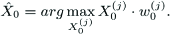
As we know, the appearance pattern based tracking algorithms are sensitive to changes in illumination and shadows. As shown in Figure 9 (a), in the experiment we manually changed the global illumination of some frames. Since saliency features are based on differences between the object and background, our algorithm successfully tracks the red car, while the result of Mean-Shift drifts obviously. When the car runs under the trees, the occlusion also changes the target's appearance. The saliency detector does not take temporal consistency into consideration, so its detection results are disturbed by occlusion. Figure 9 (c) shows the F-measure curves of the three algorithms. From the F-Measure curve we can see that the Mean-Shift only achieves good results in the first few frames. The saliency detector's performance is unstable: very good in the beginning and the ending parts of the video clip, but very bad between frame #20 and #80 when the scene becomes dark and the car is covered by trees. However, our approach has a temporal coherency constraint, so its performance is stable in the video clip.

Figure 9.

Object discovery and tracking under hard conditions. (a) shows the results of frame #1, #46, #58 and #78 in the car sequence. (b) shows the results of frame #1, #46, #58 and #78 in the snowboard sequence. Green dot-dash boxes are the results of D1; Blue thick dash boxes are the results of D2; Red solid boxes are the results of D3, which are our results. (c) F-measure curve comparison between the 3 approaches. Curves on left and right correspond to the car sequence and the snowboard sequence respectively. (figure best seen in colour).

We also run our algorithm under the condition when an object's pose changes a lot. As in Figure 9 (b), when the player jumps, his body stretches strenuously and causes severe incoherence between frames. Moreover, pose changing also causes unpredictable changes in the object's shape and appearance colour. The Mean-Shift algorithm totally fails in some frames, while our algorithm is robust to the change of the object's pose and scale and so does the saliency detector algorithm.

However, the saliency detector sometime includes the crowd or the commercial board in the salient area. From the F-Measure curves shown in Figure 9 (c) we can see our algorithm achieves plausible results in most of the frames, while the saliency detector performs well only in some of the frames and the Mean-Shift algorithm loses the object in most of the frames.

Figure 10 shows the comparison of our approach with D1 and D2 on the whole AIAR-SoT database. Notice that D1 performs badly on our database. The reasons are two-fold: first, the Mean-Shift algorithm we are using does not tolerate size change; second, the appearance of objects usually changes with their pose, which makes it hard to verify them with the initial model. Our approach also outperforms D2 in all the criterions except precision because results of D2 tend to contract part of the object. Our approach may have a similar problem, but this only appears when the object is very big. Notice this contraction problem also make the recall of D2 lower. Compared with D2, our approach improves the F-measure by 18.5% and reduces BDE by 29.9%.

Figure 10.

Comparison with different approaches. In (a) and (b) 1–3 corresponds to approach D1-D3 respectively.

To make the comparison more extensive, we also run our approach on the dataset, which is used in [29]. Figure 11 demonstrates some results and compares the precision, recall and F-measure of our approach and that in [29]. We can see that our approach outperforms the comparison one by 4.5% on the F-Measure.

Figure 11.

(a) shows some of our tracking results on the dataset proposed by Liu in [29]. (b) is the comparison of Liu's approach (shown as 1) and our approach (shown as 2) on precision, recall, and f-measure.

4.5 Key object Extraction

We perform the key object extraction on the subset of our database where we have labelled the object segmentation mask. In our implementation, to avoid the case that the bounding box doesn't cover the whole object, we expand the bounding box by 15%.

We compare our results with two baselines.

S1: The first baseline is GrabCut+Saliency. GrabCut [34] is a segmentation method with a bounding box prior. However, this approach is only based on the colour similarity and does not achieve comparable results on our data. To make it more competitive, we use our saliency map to further guide the segmentation. Inside the bounding box, we compute Otsu's threshold and find the area where the saliency value is lower than 70% of the threshold. We believe this area is definitely background. When we do GrabCut, we remove this area from the foreground marking and add it to background marking.

S2: The other baseline is a relatively simple one, which is carrying out object segmentation on the saliency map using Otsu's threshold.

S3: The proposed approach in this paper.

Figure 12 (a)-(b) show the original frames and the results of approaches S1-S3. Our approach extracts the object boundary correctly even in some very hard cases. For example, in the “ridehorse6” sequence, the boundary on the head of the horse is very faint, which makes it difficult to cut using regular approaches. However, our Gabriel graph based super-pixel bridges the gaps and our saliency map provides clear information on object-background assignment.

Figure 12.

The key object segmentation comparison between our approach and the baselines. (a) shows some results of the 'Snowboard1’ sequence. (b) shows some results of the ‘ridehorse6’ sequence. In (a) and (b), from left to right are original frames, results of S1, S2 and S3. (c) shows the criteria comparison between these approaches. 1–3 correspond to S1-S3 respectively.

From the results we can also see that even the naive approach S2 achieves acceptable segmentation. This is because our saliency map clearly indicates the key object area where all the pixels inside the object have much higher saliency values than the pixels on the background. It is impossible to extract the object from many other saliency maps with such a simple binarization approach.

Figure 12 (c) shows the precision, recall and f-measure criteria comparison between the three approaches. Our performance on precision and f-measure are the highest, as expected. The other two approaches have higher recalls but they always leak to the background. This is also the reason why their precisions are low.

5. Conclusion and Future Work

In this paper, we propose an on-line system to discover and track the key object in a video clip. The basic idea is to use static and dynamic saliency information to detect and track the object. To further improve the performance of the saliency maps, we propose a context-aware saliency computation mechanism. This mechanism takes the spectral neighbours of each pixel and refines the saliency of the pixel, considering the saliency of all its neighbours. By using context-aware computation, our saliency maps become more discriminative. To detect and track the key object, we adaptively combine the static and dynamic saliency map and perform the sequential Monte-Carlo sampling method. Finally, to make the result more accurate, we further perform a super-pixel based 3D-GraphCut inside the tracked bounding box to extract the object boundary. To evaluate the robustness and efficiency of our approach, we built a well-labelled salient object tracking database. The performance of our method is compared with those of other methods proposed in the literature. From the experimental results, we confirmed that our approach achieves more accurate tracking and segmentation on key objects. Therefore, we believe that our work provides a reasonable starting point for plenty of applications, such as video summarization, action recognition, video indexing and so on.

There are several possible remaining issues for further investigation. One of the problems is multiple key objects detection and tracking. Some articles have proposed methods to detect multiple objects on an image. In the future, we plan to improve our tracking model by using constraints such as colour histograms and state space continuity for multiple targets association. Another potential improvement is predicting the reliability of static and dynamic saliency features in advance. By doing so, when only one kind of the features is reliable, we do not need to compute the other saliency map.

Footnotes

6. Acknowledgements

This work was supported in part by the National Basic Research Program of China under Grant No. 2012CB316400, and the National Natural Science Foundation of China under Grant No. 91120006.

References

Lopez

M. T.

Fernandez

(2006) Visual surveillance by dynamic visual attention method. Pattern Recognition, vol. 39(11), pp. 2194–2211.

Itti

(2004) Automatic foveation for video compression using a neurobiological model of visual attention. IEEE Trans. Image Process., vol. 13(10), pp. 1304–1318.

Cheng

W.-H.

Wang

C.-W.

J.-L.

(2007) Video adaptation for small display based on content recomposition. IEEE Trans. Circuits Syst. Video Techn., vol. 17, no. 1, pp. 43–58.

Liu

Sun

Zheng

Tang

Shum

(2007) Learning to detect a salient object. IEEE Conf. on Computer Vision and Pattern Recognition, pp. 1–8.

Mahadevan

Vasconcelos

(2009) Saliency-based discriminant tracking. IEEE Conf. on Computer Vision and Pattern Recognition, pp. 1007–1013.

Liu

Zheng

Ding

Yuan

(2008) Video attention: Learning to detect a salient object sequence. IEEE Int. Conf. on Pattern Recognition, pp. 1–4.

Mahadevan

Vasconcelos

(2010) Spatiotemporal saliency in dynamic scenes. IEEE Trans. Pattern Anal. Mach. Intell., vol.21(1), pp. 171–177.

Brox

Bruhn

Papenberg

Weickert

(2004) High accuracy optical flow estimation based on a theory for warping. European Conf. on Computer Vision, vol. 4, pp. 25–36.

Zhang

Yuan

Zheng

Sheng

Liu

(2009) Visual saliency based object tracking. in Proc. Asian Conf. on Computer Vision, 2009.

10.

Matula

D. W.

Sokal

R. R.

(1980) Properties of Gabriel graphs relevant to geographic variation research and the clustering of points in the plane. Geographical Analysis, vol. 12(3), pp. 205–222.

11.

Chew

L. P.

(1989) Constrained Delaunay triangulations. Algoritmica, vol. 4(1), pp. 97–108.

12.

Isard

Blake

(1998) Condensation: Conditional density propagation for visual tracking. Int. J. Comput. Vision, vol. 29(1), pp.5–28.

13.

Comaniciu

Ramesh

Meer

(2000) Real-time tracking of non-rigid objects using mean shift. IEEE Conf. Computer Vision and Pattern Recognition, pp. 142–149.

14.

Rasmussen

Hager

G. D.

(2001) Probabilistic data association methods for tracking complex visual objects. IEEE Trans. Pattern Anal. Mach. Intell., vol. 23(6), pp. 560–576.

15.

Comaniciu

Ramesh

Meer

(2003) Kernel-based object tracking. IEEE Trans. Pattern Anal. Mach. Intell, vol. 25(5), pp. 564–577.

16.

Gordon

N. J.

Salmond

D. J.

Smith

(1993) Novel approach to nonlinear/non-Gaussian Bayesian state estimation. IEE Proc. on Radar and Signal Process., vol. 140, pp. 107–113.

17.

Boykov

Huttenlocher

(2000) Adaptive Bayesian recognition in tracking rigid objects. IEEE Conf. on Computer Vision and Pattern Recognition, pp. 697–704.

18.

Perez

Hue

Vermaak

Gangnet

(2002) Color-based probabilistic tracking. European Conf. on Computer Vision, pp. 661–675.

19.

Mansouri

A. R.

(2002) Region tracking via level set PEDs without motion computation. IEEE Trans. Pattern Anal. Mach. Intell, vol. 25(7), pp. 947–961.

20.

Ross

Lim

Yang

(2004) Adaptive probabilistic visual tracking with incremental subspace update. European Conf. on Computer Vision, pp. 470–482.

21.

Matthews

Ishikawa

Baker

(2004) The template update problem. IEEE Trans. Pattern Anal. Mach. Intell, vol. 26(6), pp. 810–815.

22.

Avidan

(2004) Support vector tracking. IEEE Trans. Pattern Anal. Mach. Intell, vol. 28(6), pp. 1064–1072.

23.

Avidan

(2007) Ensemble tracking. IEEE Trans. Pattern Anal. Mach. Intell, vol. 29(2), pp. 261–271.

24.

Collins

R. T.

Liu

Leordeanu

(2005) Online selection of discriminative tracking features. IEEE Trans. Pattern Anal. Mach. Intell, vol. 27(10), pp. 1631–1643.

25.

Yang

Yuan

(2007) Spatial selection for attentional visual tracking. IEEE Conf. Computer Vision and Pattern Recognition, pp. 1–8.

26.

Y. F.

Zhang

H. J.

(2003) Salient region detection and tracking. IEEE Int. Conf. on Multimedia and Expo., vol. 2, pp. 269–272.

27.

Goferman

Zelnik-Manor

Tal

(2010) Context-aware saliency detection. IEEE Conf. Computer Vision and Pattern Recognition, pp. 2376–2383.

28.

Wang

Loe

K.-F.

J.-K.

(2006) A dynamic conditional random field model for foreground and shadow segmentation. IEEE Trans. Pattern Anal. Mach. Intell, vol. 28(2), pp. 279–289.

29.

Liu

Yuan

Sun

Wang

Zheng

Tang

Shum

(2011) Learning to detect a salient object,” IEEE Trans. Pattern Anal. Mach. Intell, vol. 33(2), pp. 353–367.

30.

Otsu

(1979) A threshold selection method from gray-level histograms. IEEE Trans. Sys., Man., Cyber., vol. 9(1), pp. 62–66.

31.

Martin

D. R.

Fowlkes

C. C.

Malik

(2004) Learning to detect natural image boundaries using local brightness, color, and texture cues. IEEE Trans. Pattern Anal. Mach. Intell., vol. 26, pp. 530–549.

32.

Freixenet

Munoz

Raba

Marti

Cufi

(2002) Yet another survey on image segmentation: Region and boundary information integration. European Conf. on Computer Vision, pp. 408–422.

33.

Blake

Rother

Brown

Perez

Torr

, (2004) Interactive image segmentation using an adaptive GMM-RF model. European Conf. on Computer Vision, pp. 428–441.

Key Object Discovery and Tracking Based on Context-Aware Saliency

Abstract

Keywords

1. Introduction

2. Related Work

3. Proposed Method

3.1 Context-Aware Saliency

3.2 Key object Tracking

3.2.1 Particle Filter

3.2.2 Observation Model

3.2.3 Initialization

3.3 Key object Segmentation

4. Experiments

4.1 Key object Segmentation

4.2 Evaluation Criteria

4.3 Context-Aware Saliency

4.4 Saliency Feature Integration

4.5 Salient object tracking comparison

4.5 Key object Extraction

5. Conclusion and Future Work

Footnotes

6. Acknowledgements

References