Sage Journals: Discover world-class research

Abstract

In this paper, we present a tracking technique utilizing a simple saliency visual descriptor. Initially, we define a visual descriptor named local similarity pattern that mimics the famous texture operator local binary patterns. The key difference is that it assigns each pixel a code based on the similarity to the neighbouring pixels. Later, we simplify this descriptor to a local saliency operator which counts the number of similar pixels in a neighbourhood. We name this operator local similarity number (LSN).

We apply the local similarity number operator to measure the amount of saliency in a target patch and model the target. The proposed tracking algorithm uses a joint saliency-colour histogram to represent the target in a mean-shift tracking framework. We will show that the proposed saliency-colour target representation outperforms texture-colour where texture modelled by local binary patterns and colour target representation techniques are used.

Keywords

Mean-shift Tracking Saliency Local Binary Patterns

1. Introduction

Texture analysis has gained lots of popularity in recent years due to its wide range of uses in industry and different machine vision applications, for instance classification of different materials or visual inspection of material surfaces. Thus different operators have been introduced over the decades to enhance texture analysis, e.g., co-occurrence matrices [1] and polarograms [2]. One of the most successful operators in this field is the local binary patterns (LBP) [3]. It is grey-scale invariant and fast to compute. This makes LBP a powerful means of texture analysis.

Local binary patterns is widely used in areas of visual inspection, image and video retrieval, aerial image analysis, environment modelling, biomedical image analysis, and biometrics. It is successfully applied for example to face and gender classification [4], paper characterization [5] and wood inspection [6], as well as background subtraction in tracking problems [7].

Different extensions exist to LBP. Ojala et al. [8] introduced a multi-resolution extension and later they enhanced it furthermore by finer quantization of angular space using uniform patterns. LBP can be modified easily to adapt to the problem of interest. These modifications can be a simple threshold modification [9] or a more sophisticated approach of incorporating feature distributions [10].

In this paper, we define a local similarity descriptor that assigns each pixel a binary pattern based on the similarity to its surrounding pixels. This operator is simplified to measure the amount of salience for each pixel by counting the number of similar pixels in the surrounding of a pixel. This will assign each pixel a number that represents how different it is to the surrounding. We utilize this simplified version of the operator to measure the amount of salience in a local window. Based on the salience value, we compute a joint saliency-colour histogram to represent a specific target in a local window. We will show that this operator outperforms target representation using joint texture-colour and colour histogram descriptors.

2. Local Similarity Operator

There has been lots of research on saliency, especially in recent years [11]. Many techniques tried to employ the centre-surround mechanism which relies on comparing a central region with its surrounding. For instance, Itti et al. [12] computed different feature channels and fused them in a centre-surround approach. Later [13] studied the characteristics of centre-surround saliency and wrote on the biological plausibility of this approach.

Getting advantage from centre-surround differences in computer vision is not limited to saliency computation. Local Binary Patterns (LBP) [14] derives advantage from the same phenomena to represent structural information from the neighbourhood of a pixel. The main idea of LBP is partitioning the surrounding pixels into those of higher intensity values and the group with lower intensity values relative to the centre. The first group will be assigned label ‘1’ and the latter one ‘0’ which can be used to assign the central pixel a binary label.

In the local similarity operator defined here, instead of partitioning pixels into the two aforementioned groups, we consider partitioning them into groups of similar and dissimilar pixels. A threshold value will be used to define the amount of similarity and surrounding pixels are considered similar to centre if they fall within this similarity threshold.

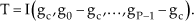
Let us start by presenting the grey-scale similarity operator by defining texture T in a local neighbourhood of a grey-scale image I:

T = I (g_{c}, g_{0}, \dots, g_{P - 1}) .

(1)

where the grey value g corresponds to the centre of neighbourhood, and g_i,(i=0,…,i=P-1) correspond to the grey values of P neighbouring pixels lying on a circle of radius R, (R > 0). P neighbouring pixels are spaced equally. In fact, the neighbourhood is circularly symmetric, similar to the LBP_P_,R neighbourhood [8].

2.1. Local Similarity Pattern

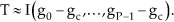
At first the grey value g_c is subtracted from the grey values of neighbourhood g_i,(i=0,…,i=P-1):

T = I (g_{c}, g_{0} - g_{c}, \dots, g_{P - 1} - g_{c}) .

(2)

In case of texture analysis, it is proven in [15] that (2) can be simplified and approximated without loss of useful information using:

T \approx I (g_{0} - g_{c}, \dots, g_{P - 1} - g_{c}) .

(3)

Since g_i - g_c is not affected by changes in the mean luminance, (3) is invariant against grey-scale shifts. If fact, it is possible to only consider the sign of differences [8]. Consequently, we introduce a similarity merit function which is invariant against grey-scale shifts and produces results similar to sign function:

T \approx I (f (g_{0} - g_{c}, d), \dots, f (g_{P - 1} - g_{c}, d)) .

(4)

where

f (x, d) = {\begin{matrix} 1, & | x | & \leq & d \\ 0, & | x | & > & d . \end{matrix}

(5)

A unique number can be obtained by transforming (4) using a binomial factor 2ⁱ for each f(g_i- g_c, d). The number obtained characterizes the similarity pattern of the local image. The obtained number is called “Local Similarity Pattern (LSP)”.

L S P_{P, R}^{d} = \sum_{i = 0}^{P - 1} f (g_{i} - g_{c}, d) 2^{i} .

(6)

The operator is called LSP because it produces a local bit pattern based on the similarity of neighbouring pixels and the centre. The proposed LSP operator produces LBP-like patterns that differ from the original local binary patterns in the respect that we produce them. Figure. 1 provides an example of how LSP and LBP will provide a different pattern given the same texture.

Figure 1.

Comparison of LBP and LSP generated patterns, (a) is a sample grey patch, (b) is the LBP generated labels that produces ‘00011101’ and (c) is the LSP generated binary labels using d = 2 that gives ‘00111001’.

2.2. Local Similarity Number

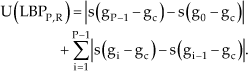
In the previous section, it was explained how a local similarity pattern can be obtained. The local similarity pattern includes the structural information of the saliency. In order to compute saliency the structural information is of no help. Hence, we can discard the structural information. This can be achieved by simply modifying (6) and replacing the binomial factor 2ⁱ with 2⁰. This reduces (6) to the following:

L S N_{P, R}^{d} = \sum_{i = 0}^{P - 1} f (g_{i} - g_{c}, d) .

(7)

which is equivalent to summing the binary codes assigned by (5) to the surrounding pixels. Hence, by calculating LSN we obtain the number of similar pixels in the local neighbourhood; as an example LSN^d_8,R = 8 means all the eight neighbouring pixels of radius R are similar to the centre considering distance d.

The local similarity number shows the pop-out property of a pixel which defines how different a pixel from its surrounding neighbourhood is. The lower the number, the more salient the central pixel is. Hence, (7) can be used to show saliency of the central pixel. Figure 2 shows the nine saliency degrees of LSN^d_8,R where (a) is the less salient and (i) is the most salient pattern.

Figure 2.

Groups of LSN_8,1 patterns, any of the 256 patterns is member of a group. Black circles represent pixels similar to the centre. (a) Has only one member where all the pixels are similar and is the representation of a flat area; (b) - (h) has several members depending on the combination of similar pixels; (i) has only one member and is the most salient pixel since all the neighbouring pixels are different.

2.3. Colour Extension

The similarity operators LSP and LSN can be easily extended to colour space. The colours are located sequentially after each other in the colour space using the Euclidean distance [16]. So, it is easy to transform proposed operators from simple grey-scale operators to colour operators. The colour texture can be represented using the following:

\begin{array}{l} T \approx t (f (g_{R 0} - g_{R c}, g_{G 0} - g_{G c}, g_{B 0} - g_{B c}, d), \dots, \\ f (g_{R P - 1} - g_{R c}, g_{G P - 1} - g_{G c}, g_{B P - 1} - g_{B c}, d)) . \end{array}

(8)

where g_Ri is the value of red channel, g_Gi represents value of green channel, and g_Bi is the value of blue channel.

f (x_{r}, x_{g}, x_{b}, d) = {\begin{matrix} 1, & \sqrt{x_{r}^{2} + x_{g}^{2} + x_{b}^{2}} & \leq & d \\ 0, & \sqrt{x_{r}^{2} + x_{g}^{2} + x_{b}^{2}} & > & d . \end{matrix}

(9)

3. Target Representation

In this section, we explain how to apply LSN and LBP to extract masks that are needed in target representation which will be used in tracking. Initially, we will explain how the saliency operator can be used to represent the target by using saliency extracting an LSN Mask. Afterwards, we will discuss the target representation method of [9]. Their method is based on textural analysis using LBP masks.

3.1. LSN Mask

In the case of $L S N_{8, R}^{d}, 2^{8}$ ⁸ patterns exist which are grouped into nine categories as shown in Figure, 2. The similarity number shows the number of the pixels in a neighbourhood that are similar, e.g., the pattern with similarity number 8 obtained from LSNd_8,R means that all neighbouring pixels are similar.

In colour-LSN target representation, the aim is preserving the unity of the target of interest as well as its edges, lines and corners. Hence, we modify LSN^d_8,1 to fulfil the required properties as follows:

m L S N_{8, 1}^{d} = {\begin{cases} 1 + \sum_{i = 0}^{7} f (g_{i} - g_{c}, d), \sum_{i = 0}^{7} f (g_{i} - g_{c}, d) \in {0, 1, 2, 3, 4} \\ 0, otherwise . \end{cases}

(10)

where $\sum_{i = 0}^{7} f (g_{i} - g_{c}, d)$ is equivalent to LSN^d_8,1. The proposed constrain assigns central pixel a value in the range of [0, 5]. Each value defines the salience measure of the central pixel; 0 means the central pixel is not salient and 1 means it is maximally salient. The other values define relative salience value. Figure 3 depicts the LSN mask for a small target patch.

Figure 3.

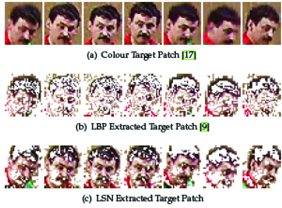
Different patch representations. LBP-colour joint histogram process patches mostly on the edges of the object as can be seen in (b). On the other hand, as (c) depicts, patches of LSN-colour joint histogram convey more useful information while suppressing background and plain areas.

3.2. LBP Mask

Recently, Ning et al. [9] presented an object tracking method using a joint colour-texture histogram which relies on the local binary pattern. The method utilizes major uniform patterns of $L B P_{8, 1}^{r i u 2}$ in a modified manner, which we refer to as modified LBP. Thus, their selected patterns can be produced using:

m L B P_{8, 1}^{r i u 2} = {\begin{cases} \sum_{i = 0}^{7} s (g_{i} - g_{c} + a) U (L B P_{8, 1}) \leq 2 and \\ \sum_{i = 0}^{7} s (g_{i} - g_{c} + a) \in {2, 3, 4, 5, 6} \\ 0 otherwise . \end{cases}

(11)

where

\begin{array}{l} U (L B P_{P, R}) = | s (g_{P - 1} - g_{c}) - s (g_{0} - g_{c}) | \\ + \sum_{i = 1}^{P - 1} | s (g_{i} - g_{c}) - s (g_{i - 1} - g_{c}) | . \end{array}

(12)

and

s = {\begin{matrix} 1 & x & \geq & 0 \\ 0 & x & < & 0 . \end{matrix}

(13)

and a are robustness terms set to 1e⁻⁶ in the experiments similar to [9].

Figure 3 shows sample masks extracted using aformentioned techniques. The masks include key feature points in the target region, obtained using (11) and (10). As seen, the smooth area (i.e., background) in both target patches are eliminated. In comparison to traditional colour representation (i.e., colour patch), both LSN and LBP extract effectively edge and corner features. The advantage of LSN is that it preserves unity of the object of interest better and saves more useful information; thus it is expected to model the target more effectively.

4. Tracking

Object tracking is a challenging task. It has a wide range of applications in different machine vision applications such as automated surveillance, video indexing, human-computer interaction and traffic monitoring. Different tracking algorithms exist which are categorized into point tracking, kernel tracking and silhouette tracking [18]. Mean-shift tracking is a kernel-based algorithm, where a kernel is the object shape and appearance that is supposed to be tracked. The object can be represented using a rectangular or elliptical patch. We applied a colour-LSN histogram for object representation in the mean-shift algorithm. This method is compared with an algorithm [9] which utilizes a colour-LBP histogram.

4.1. Mean-shift Algorithm

Suppose the normalized target patch is represented by {x^*₁}_i=1…n. The target model is computed as follows:

{\begin{cases} \overset{⌢}{q} = {{\overset{⌢}{q}}_{u}}_{u = 1 \dots m} \\ {\overset{⌢}{q}}_{u} = C \sum_{i = 1}^{n} k ({‖ x_{i}^{*} ‖}^{2}) δ ([b (x_{i}^{*}) - u]) \\ C = 1 / \sum_{i = 1}^{n} k ({‖ x_{i}^{*} ‖}^{2}) . \end{cases}

(14)

where ${\overset{⌢}{q}}_{u}$ represents the probability of feature u in target model $\overset{⌢}{q}$ , m is the number of bins, δ is the Kronecker delta function, b(x_i*) associates the pixel with the histogram, and K(x) is an isotropic kernel profile.

The candidate model $\overset{⌢}{p} (y)$ of candidate region {x_i}_i=1…n is computed similarly as follows:

{\begin{cases} \overset{⌢}{p} (y) = {{\overset{⌢}{p}}_{u} (y)}_{u = 1 \dots m} \\ {\overset{⌢}{p}}_{u} (y) = C \sum_{i = 1}^{n} k ({‖ \frac{y - x_{i}}{h} ‖}^{2}) δ ([b (x_{i}) - u]) \\ C = 1 / \sum_{i = 1}^{n} k ({‖ \frac{y - x_{i}}{h} ‖}^{2}) . \end{cases}

(15)

where ${\overset{⌢}{p}}_{u} (y)$ is the probability of feature u, h is the bandwidth and y is the centre of candidate region.

It is proven in [17] that in order to estimate the new position y from position y iteratively we can use

{\begin{cases} \overset{⌢}{y} = \frac{\sum_{i = 1}^{n} x_{i} w_{i}}{\sum_{i = 1}^{n} w_{i}} \\ w_{i} = \sum_{u = 1}^{m} \sqrt{\frac{{\overset{⌢}{q}}_{u}}{{\overset{⌢}{p}}_{u} (y)}} δ ([b (x_{i}^{*}) - u]) . \end{cases}

(16)

4.2. Tracking Using a Joint Colour-Texture Histogram

We use RGB channels and mLSN patterns obtained from (10) to jointly represent the target and apply it in the mean-shift algorithm. In order to do this, the target model $\overset{⌢}{q}$ distribution is approximated using a colour and LSN texture histogram. The histogram consists of 8-bin quantized colour RGB channels and 5-bin saliency information of mLSN which makes the histogram of size 8 × 8 × 8 × 5. The whole tracking mechanism for one frame is summarized in the following algorithm.

Input: A target model

\overset{⌢}{q}

, location of target y from previous frame, ϵ minimum distance between target models and maximum iteration N. Output: Target location in current frame

\overset{⌢}{y}

. 1: Initialize iteration number t ← 0. 2: repeat 3: compute

\overset{⌢}{q} (y)

using (15) 4: compute

\overset{⌢}{y}

using (16) 5:

d \leftarrow ∥ \overset{⌢}{y} - y ∥, y \leftarrow \overset{⌢}{y}, t \leftarrow t + 1

6: until t < N and ϵ < d

Algorithm 1. Tracking algorithm

In the case of a colour-LBP, the joint-histogram consists of 8-bin quantized colour RGB channels and 5-bin mLBP texture information obtained from (11); the same procedure described above applies.

5. Experimental Results

In this section, experiments are conducted to show the performance of the mean-shift-based tracking algorithms using different target representation methods. Three target representation models are tested, the first one uses an RGB histogram as explained in [17]. The second algorithm [9] utilizes the mLBP to form a joint colour-LBP histogram. The third algorithm uses the proposed mLSN operator to build the joint colour-LSN histogram. They are referred to as T₁, T₂ and T₃ respectively.

The algorithm is implemented using MATLAB 2008a and run on a computer with a 2.4 GHz Intel Core2 Duo P8600 CPU and 4GB RAM. The operating system is Windows Vista SP2.

Quantitative assessments are done using PETS2001 (available at http://ftp.pets.rdg.ac.uk/PETS2001) data set. It consists of five multi-view (two camera) sequences of people and vehicles. The first sequence with the first camera is used in our experiments. The aim of these experiments is tracking people. Tracking started when the target is completely in a frame and stopped before leaving in final frames. Error is calculated from centroid deviation using the available ground truth (annotation).

In the first experiment, a walking boy crossing from left to right is tracked. He is wearing a green shirt that is similar in colour to the grass he is walking on. In the middle of the sequence he is occluded by a lamppost and walks on a road that is similar in colour to his trousers. Figure 4 shows the tracking trajectory for each target model. Table 1 summarizes tracking information, including standard deviation of error, number of iterations, average iterations per frame and computation time. Computation time is estimated using tic/toc commands in MATLAB.

Figure 4.

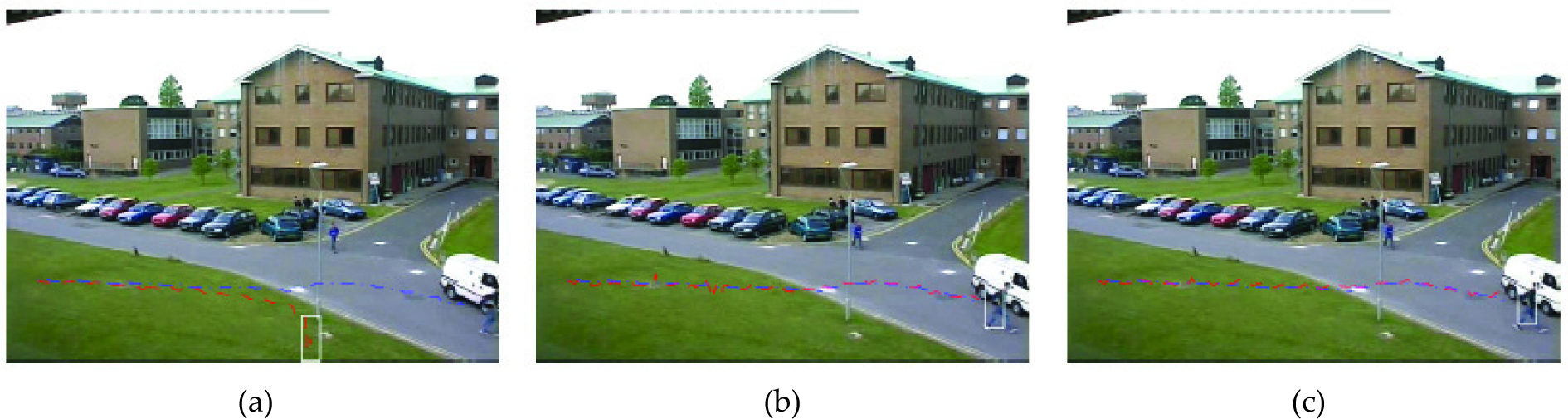
Tracking trajectory for boy in green shirt. Target video sequence has 261 frames (used frames: 10–251). Blue trajectory is the ground-truth. (a) RGB model, misses target on frame 151. (b) RGB-LBP model. (c) RGB-LSN model.

Table 1.

Tracking result for boy in green shirt. Number of frames processed is 241 out of 261 (frames: 10–251)

	Target Model
	T1 [17]	T2[9]	T3
Error standard deviation	80.0733	2.6392	2.3257
Number of iterations	1027	853	756
Average iteration per frame	4.0916	3.5394	3.1136
Computation time (sec)	169.1716	1145.4227	290.5509
Missed target frame number	151	—	—

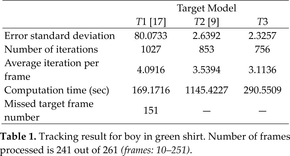
The first experiment shows that using T1, the mean-shift algorithm is not accurate and can easily miss the target. On the other hand, T2 is robust against missing the target. However, it is not as accurate as T3. As shown in Table 1, the target representation using T3 has the lowest error standard deviation.

Another factor that is useful for evaluation of the efficiency of the mean-shift-based tracking algorithm is number of iterations. The lower the iteration number, the faster the convergence speed. As shown in this experiment, T3 outperforms the others having to iterate only 756 times.

The second experiment tries to follow a woman in cream shirt. She is accompanied by a man in a white shirt. They start walking along the road from right to the left. The purpose of this experiment is to test the robustness in partial occlusion situations. The man is in front. The sequence has 513 frames, from which only 90 frames are processed. T1, and T2 both miss the woman in frame 37. However, T3 continues tracking with no difficulty. Figure 5 shows the trajectory for the processed frames. The tracking result is summarized in Table 2.

Figure 5.

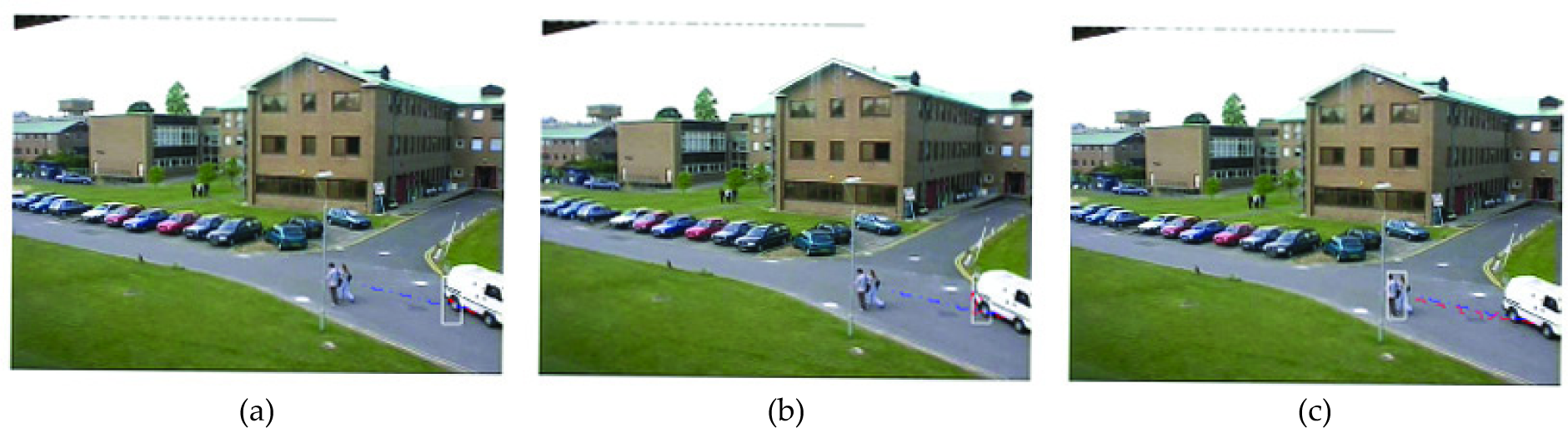
Tracking trajectory for the woman in cream shirt. Target video sequence has 513 frames (used frames: 10–100). Blue trajectory is the ground-truth. (a) RGB model, misses target on frame 37. (b) RGB-LBP model, misses target on frame 37. (c) RGB-LSN model.

Table 2.

Tracking result for the woman in cream shirt. Number of frames processed is 90 out of 513

	Target Model
T1[17]	T2[9]	T3
Error standard deviation	53.7381	51.0357	4.5935
Number of iterations	240	345	404
Average iteration per frame	2.6667	3.8333	4.4889
Computation time (sec)	70.8241	394.7055	106.2753
Missed target frame number	37	37	—

(frames: 10–100)

Considering Table 2, it is inferred that T3 is more robust against occlusion than the two other target model representation methods. It does not miss the target. However, the accuracy is not satisfactory and the tracker is biased toward the man.

Iteration number of T3 is higher than the other two methods. This is due to the adaptive nature of the LSN operator which helps in not missing the target in this experiment.

In the third experiment, the purpose is to track a woman who enters from the left and walks to the right along the road. The main goal is testing the robustness of modelling methods against continuous changes of the background. Unfortunately, all the three modelling methods fail to follow the target. T1 misses the woman after 14 frames. T2 misses the target after 45 frames, and T3 after 78 frames. Figure 6 shows the result. Although all the model representation methods miss the target, it takes a longer time for T3 to miss the target. All the above experiments show the proposed method is accurate and fast in comparison with the two other methods.

Figure 6.

Tracking trajectory for red-shirt woman. (a) RGB model, misses target on frame 14. (b) RGB-LBP model, misses target on frame 45. (c) RGB-LSN model, misses target on frame 786.

6. Conclusion

In this paper a visual similarity operator based on LBP was introduced. The operator uses a similarity measure function to produce binary patterns. We extended the operator to simply measure the amount of saliency. This new variation simply counts the number of similar to centre pixels, so it was named local similarity number (LSN).

The operator was applied to object tracking in the mean-shift algorithm. The target was modelled by extracting a mask using LSN and computing a joint colour-LSN histogram within that mask. This target representation effectively suppresses the smooth area in the target patch while preserving edges and corners as well as target unity.

The proposed model was compared with original colour-histogram modelling [17] and colour-LBP modelling [9]. The experiments showed that this new operator produces excellent tracking results and outperforms the other two modelling methods. Moreover, it convergences faster than the other models.

References

Davis

L. S.

Johns

S. A.

, and Aggarwal

J. K.

. Texture analysis using generalized cooccurence matrices. IEEE Trans. Pattern Anal. Mach. Intell., 1:251–259, 1979.

Davis

L. S.

. Polarograms: A new tool for image texture analysis. Pattern Recognition, 13:219–223, 1981.

Mäenpää

Viertola

, and Pietikäinen

. Optimising colour and texture features for real-time visual inspection. 2003. Pattern Analysis and Applications 6 (3):169–175.

Hadid

and Pietikäinen

. Combining appearance and motion for face and gender recognition from videos. Pattern Recognition 42 (11):2818–2827, 2009.

Turtinen

Pietikäinen

, and Silven

. Visual characterization of paper using isomap and local binary patterns. 2006. IEICE Transactions on Information and Systems E89D (7):2076–2083.

Maenpaa

. The local binary pattern approach to texture analysis extentions and applications. PhD thesis, Infotech Oulu and Department of Electrical and Information Engineering, University of Oulu, 2003.

Heikkilä

Marko

and Pietikäinen

Matti

. A texture-based method for modeling background and detecting moving objects. IEEE Trans. Pattern Anal. Mach. Intell., 28 (4):431–438, 2006.

Ojala

Timo

Pietikäinen

Matti

, and Mäenpää

Topi

. Multiresolution gray-scale and rotation invariant texture classification with local binary patterns. IEEE Trans. Pattern Anal. Mach. Intell., 24 (7):971–987, 2002.

Ning

Jifeng

Zhang

Lei

Zhang

David

, and Wu

Chengke

. Robust object tracking using joint color-texture histogram. International Journal of Pattern Recognition and Artificial Intelligence, 23 (7):1245–1263, 2009.

10.

Chen

Kan-Min

and Chen

Shu-Yuan

. Color texture segmentation using feature distributions. Pattern Recognition Letters, 23 (7):755–771, 2002.

11.

Borji

Ali

and Itti

Laurent

. State-of-the-art in visual attention modeling. IEEE Transactions on Pattern Analysis and Machine Intelligence, 99 (PrePrints), 2012.

12.

Itti

Koch

, and Niebur

. A model of saliency-based visual attention for rapid scene analysis. Pattern Analysis and Machine Intelligence, IEEE Transactions on, 20 (11): 1254–1259, nov. 1998.

13.

Gao

Dashan

Mahadevan

Vijay

, and Vasconcelos

Nuno

. On the plausibility of the discriminant center-surround hypothesis for visual saliency. Journal of Vision, 8 (7), 2008.

14.

Ojala

Timo

. Nonparametric texture analysis using spatial operators, with applications in visual inspection. PhD thesis, 1997.

15.

Ojala

Timo

Valkealahti

Oja

Pietikäinen

Matti

, and Xu

. Texture discrimination with multi-dimensional distributions of signed gray level differences. Pattern Recognition, 34:727–739, 2001.

16.

Porebski

Vandenbroucke

, and Macaire

. Haralick feature extraction from lbp images for color texture classification. pages 1–8, 2008.

17.

Commaniciu

Ramesh

, and Meer

. Kernel-based object tracking. IEEE Trans. Pattern Anal. Mach. Intell., 25 (5):564–575, 2003.

18.

Yilmaz

Alper

Javed

Omar

, and Shah

Mubarak

. Object tracking: A survey. ACM Computing Surveys, 38 (14), 2006.

Local Similarity Number and its Application to Object Tracking

Abstract

Keywords

1. Introduction

2. Local Similarity Operator

2.1. Local Similarity Pattern

2.2. Local Similarity Number

2.3. Colour Extension

3. Target Representation

3.1. LSN Mask

3.2. LBP Mask

4. Tracking

4.1. Mean-shift Algorithm

4.2. Tracking Using a Joint Colour-Texture Histogram

5. Experimental Results

6. Conclusion

References