Human Long Jump — A Deductive Approach

Abstract

This paper presents a useful application of a generalized approach to the modelling of human and humanoid motion using the deductive approach. It starts with formulating a completely general problem and deriving different real situations as special cases. The concept and the software realization are verified by comparing the results with the ones obtained using “classical” software for one well-known particular problem – biped walking. New applicability and potentials of the proposed method are demonstrated by simulation of a selected example – the long jump. The simulated motion included jumping and landing on the feet (after a jump). Additional analysis is done in the paper regarding the joint torque and joint angle during the jumping. Separate stages of the simulation are defined and explained.

Keywords

Humanoid dynamics contact task impact human motion Zero-Moment Point (ZMP)

1. Introduction

Using a general model of human motion, this paper presents a human long jump simulation. This new idea, proposed in [1], was called the “deductive approach”. Bipedal gait has widely been elaborated upon (originally starting from [1 -5]) and jumping and running have been solved recently [6]. A very different model was developed for a rather different motion – somersaults on the trampoline [7, 8]. A review of advanced topics in humanoid dynamics can be found in [4]. One may note that for these particular problems, separate models were developed. If specific models were derived for different problems, such as gymnastic exercises, soccer or tennis, then it would be a huge problem to make a generalization. The deductive approach [1] follows a deductive principle: we derive a general model and consider all mentioned particular motions as being just special cases. Contact analysis, essential in this method, has been also explained in [1]. Landing analysis are presented in [9, 10]. Pose has already been analysed in [11 -13].

According to [1], the general approach is based on an articulated system (e.g., a human body, a humanoid, or even an animal) that “flies” without constraints (meaning that it is not connected to the ground or to any object in its environment – see Fig. 1). For this the term flier was suggested. Such a situation is not uncommon in reality (it is present in running, jumping, trampoline exercises, etc.), but it is less common than the motion where the system is in contact with the ground or some other supporting object in its environment (e.g., single- and double-support phases of walking, gymnastics on some apparatuses, etc.)

Figure 1.

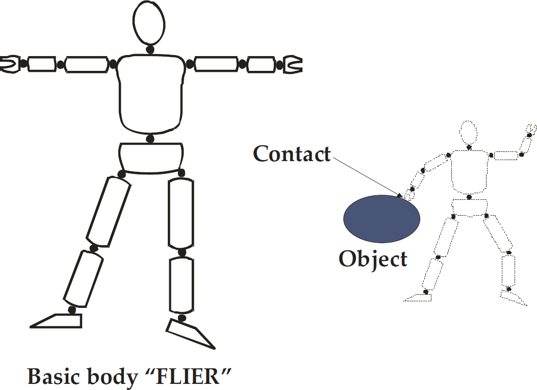
Unconstrained system – free flier.

2. Model basement

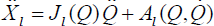
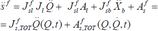
A detailed description of the deductive approach is presented in [1] and here we will describe in brief only some important notions regarding the specific task of the long jump motion. The deductive approach is based on a general model human/humanoid system positioned in space without any constraints, called “flier” (Figure 1.) In the deductive approach we use the dynamic model of the free flier in the general form:

H (Q) \ddot{Q} + h (Q, \dot{Q}) = Τ

(1)

where Q object position is defined by his internal coordinate. The dimensions of the inertial matrix and its submatrices are: H(N × N), H_X,X(6×6), H_X,q(6×n), H_q,X(n×6), and H_q,q(n×n). The dimensions of the vectors containing centrifugal, Coriolis' and gravity effects are: h(N), h_X(6), and h_q(n).

In our model we use a human/humanoid model having n = 20 DOFs at its joints as shown in Figure 2. This can be seen as a humanoid or an approximation of the human body. The definition of the joint (internal) coordinates, vector q = [q₁,···, q_n] ^T , is also presented.

Figure 2.

Configuration of the human system used in the simulation.

The task is selected as a specific long jump action going forward. A player jumps forward and lands on his feet. As stated above, for the purpose of simulation the reference motion was not measured but synthesized numerically. Here, we do not show the reference; the realized motion is considered sufficient information.

The human/humanoid is equipped with actuators at its joints and the control system that will try to track the reference motion. The local PD regulator is implemented as a control strategy:

τ_{j} = K_{P j} (q_{j} - q_{j} *) + K_{D j} {\dot{q}}_{j}, j = 1, \dots, n,

where q_j is the actual value of a joint coordinate and q_j*(t) is its prescribed reference.

In the next example, in a long jump, the external object is immobile (the ground). Note that the contact might be an inner one – involving two links of the considered system.

In order to express the coming contact mathematically, we describe the motion of the considered link by an appropriate set of coordinates. Since the link is a body moving in space, it is necessary to use six coordinates. Let this set be s = [s₁,···, s₆] ^T and let us call them functional coordinates (often referred to as s-coordinates). Functional coordinates are introduced as relative ones, defining the position of the link with respect to the object to be contacted. Several illustrative examples of s-coordinates were shown in [1]. Each choice was made in accordance with the expected contact – to support its mathematical description.

A consequence of the rigid link-object contact is that the link and the object perform some motions, along certain axes, together. These are constrained (restricted) directions. Let there be m such directions, m being a characteristic of a particular contact. Relative position along these axes does not change. Along other axes, relative displacement is possible. These are unconstrained (free) directions. In order to get a simple mathematical description of the contact, s-coordinates are introduced so as to describe relative position. Zero value of some coordinate indicates the contact along the corresponding axis. For a better understanding, we use a well-known example – the contact of the robot foot and the ground (Figure 3). We may distinguish several situations. The heel contact (Figure 3a) restricts five s-coordinates, leaving one free (thus, m = 5). The full-foot contact (Figure 3b) restricts all six coordinates (m = 6). Finally, if the robot is falling down by rotating about the foot edge (Figure 3c), then again m = 5.

Figure 3.

Different contacts of the humanoid foot and the ground. The superscript “c” indicates constrained (restricted) coordinates, while “f” indicates the free ones.

In a general case the motion of the external object (to be contacted) has to be known (or calculated from the appropriate mathematical model) and then the s-frame fixed to the object is introduced to describe the relative position of the link in the most appropriate way. In the case of an inner contact (two links in contact), one link has to play the role of the object. Thus, in a general case, the s-frame is mobile. As the link is approaching the object, some of the s-coordinates reduce and finally reach zero. The zero value means that the contact is established. These functional coordinates (which reduce to zero) are called restricted coordinates and they form the subvector s^c of dimension m. The other functional coordinates are free and they form the subvector s^f of dimension 6 – m. Now one may write:

{[s^{c}, s^{f}]}^{T} = s or {[s^{c}, s^{f}]}^{T} = K s

(2)

where K is a 6 × 6 matrix used, when necessary, to rearrange the functional coordinates (elements of the vector s) and bring the restricted ones to the first positions.

It is obvious that there are several types of possible contacts between the two bodies. One contact will restrict some s-coordinates while the other will restrict a different set. Different links may establish a contact. In different tasks, the same link will establish different contacts with different objects. For each example, a specific s-frame is needed. So, in order to arrive at a general algorithm, we have to describe link motion in a general way and, once the expected contact is specified, relate this general interpretation to the appropriate s-frame.

The general description of the link motion assumes the three Cartesian coordinates of a selected point of the link plus the three orientation angles: X_l = [x_l, y_l, z_l, θ_l, ψ_l] ^T , the subscript l standing for “link”. These are absolute external coordinates. The relation between the link coordinates X_l and the system position vector Q is straightforward:

X_{l} = X_{l} (Q)

(3)

{\dot{X}}_{l} = J_{l} (Q) \dot{Q}

(4)

{\ddot{X}}_{l} = J_{l} (Q) \ddot{Q} + A_{l} (Q, \dot{Q})

(5)

where $J_{l} = \frac{\partial X_{l}}{\partial Q}$ is a 6 × N Jacobian matrix and $A_{l} = \frac{\partial^{2} X_{l}}{\partial Q^{2}} {\dot{Q}}^{2}$ is a 6-dimensional adjoint vector.

Now let us concentrate on the object. In different examples, the same object will be contacted in a different way). Now, consider the ground (as an example of an immobile object); in walking or jumping, one type of contact of the foot and the ground exists, while in ice-skating the contact will be of a rather different kind. In a general case, the object is mobile, so, its position is described by the absolute external coordinates: X_b = [x_b, y_b, z_b, θ_b, φ_b, ψ_b] ^T , the subscript b standing for “object”.

When the s-frame is introduced to define the relative position of the link with respect to the object, the coordinates will depend on both X_b and X_l:

s = s (X_{l}, X_{b})

(6)

or in the Jacobian form:

\dot{s} = J_{s l} {\dot{X}}_{l} + J_{s b} {\dot{X}}_{b}

(7)

\ddot{s} = J_{s l} {\ddot{X}}_{l} + J_{s b} {\ddot{X}}_{b} + A_{s} .

(8)

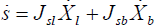
where dimension of all Jacobi matrices is 6 × 6 and the dimension of the adjoint vector A_s is 6.

Model (8) can be rewritten if the separation (2) is introduced. The model becomes

{\ddot{s}}^{c} = J_{s l}^{c} {\ddot{X}}_{l} + J_{s b}^{c} {\ddot{X}}_{b} + A_{s}^{c}

(9)

{\ddot{s}}^{f} = J_{s l}^{f} {\ddot{X}}_{l} + J_{s b}^{f} {\ddot{X}}_{b} + A_{s}^{f} .

(10)

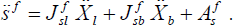
Suppose that the object motion, X_b(t) in Equations (6)–(8), is either prescribed or calculated from a separate mathematical model of the object. Equations (9) and (10) can be rewritten if (5) is introduced:

\begin{array}{l} {\ddot{s}}^{c} = J_{s l}^{c} J_{l} \ddot{Q} + J_{s l}^{c} A_{l} + J_{s b}^{c} {\ddot{X}}_{b} + A_{s}^{c} = \\ = J_{s, T O T}^{c} (Q, t) \ddot{Q} + A_{s, T O T}^{c} (Q, \dot{Q}, t) \end{array}

(11)

\begin{array}{l} {\ddot{s}}^{f} = J_{s l}^{f} J_{l} \ddot{Q} + J_{s l}^{f} A_{l} + J_{s b}^{f} {\ddot{X}}_{b} + A_{s}^{f} = \\ = J_{s, T O T}^{f} \ddot{Q} (Q, t) + A_{s, T O T}^{f} (Q, \dot{Q}, t) \end{array}

(12)

where the model matrices are: $J_{s, T O T}^{c} = J_{s l}^{c} J_{l}$ , $A_{s, T O T}^{c} = J_{s l}^{c} A_{l} + J_{s b}^{c} {\ddot{X}}_{b} + A_{s}^{c}$ , $J_{s, T O T}^{f} = J_{s l}^{f} J_{l}$ , $A_{s, T O T}^{f} = J_{s l}^{f} A_{l} + J_{s b}^{f} {\ddot{X}}_{b} + A_{s}^{f}$

An example would be walking on the ground, i.e., contact between the foot and the ground or jumping. The ground is the large immobile object. Equations (11) and (12) apply for this first case. Division of contacts can be done based on the existence of deformations in the contact zone. If there is no deformation, i.e., if the motions of the two bodies are equal in the restricted directions, then we talk about the rigid contact. If deformation is possible, then the motions in the restricted directions will not be equal. Theoretically, they will be independent, but in reality they will be close to each other, due to the action of strong elastic forces. In this case, we talk about the soft contact. This is the situation during the long jump.

The other class represents the instantaneous, short-lived contacts. When the two bodies touch each other, a short impact occurs, and after that the bodies disconnect.

The main parameters of the human/humanoid are given in Table 1. The most important is that its total weight (mass) is 70 kg. The arms (upper arm, forearm and hands) do not contribute to the total height. There are two thighs, shanks, feet, upper arms and forearms (and hands), while only one trunk and pelvis. The total mass is the sum of all segment masses.

Table 1.

Structural and dynamic parameters of the human/humanoid jumper (only the non-zero mass segments are listed).

segment	width (m)	height (m)	mass (kg)
trunk total – pelvis to head top	0.4	0.64	30.85
trunk – pelvis to shoulders	0.4	0.4
pelvis	0.27	0.15	6.96
thigh		0.44	8.41
shank		0.42	3.21
foot	0.1	0.1	1.53
forearm		0.308	2.07
upper arm		0.264	1.14
total	0.4	1.75	70.53

3. Simulation results

Figure 1 shows the realized motion of the jumper. His intention (and reference) was to jump and land. According to Fig. 1, his attempt was successful. Let us analyse the jumper's motion in more detail. One can observe several phases of the motion:

Phase 1 – take off. Both legs are in contact with the ground accelerating the body upward (Figs. 1 a, b, c). This phase ends at 0.153 s. At this instant the legs lose the contact with the ground (Fig. 1c).

• From the viewpoint of mechanics, the jumper has two contacts with an immobile object – both feet are on the ground. A closed chain is formed. Each contact restricts all six relative motions and, accordingly, creates six reaction forces/torques (twelve reactions in total).

Phase 2 – free flight. The jumper is moving (flying) up while expecting the contact with the ground. In this phase, there is no contact with any object; a true flier is considered. The system has a tree structure (no closed chain).

Phase 3 – falling down. The jumper falls down. The contact with the ground is established at 0.685 s (Fig. 1l). The landing is performed correctly, so the jumper will no overturn. In reality however, the jumper usually overturns because this extends the distance of the jump. If we are not intending to ensure dynamic balance of the system during the falling down, we will certainly extend the distance of the jump.

Our analyses will stop when the player touches the ground, but we have to note that after touching ground the simulation continues and shows that the player falls down. In the simulation the falling procedure is not analysed because it is not important for the further analysis.

We have to mention that several procedures of falling are possible including, fall forward, fall side and wall backward. Each falling procedure could be analysed in the future regarding minimizing the contact force between the ground and link in contact with the ground. This is a separate problem and could be analysed in the future, in particular, how to obtain a longer jump regarding the restriction in the take off launching force and the angle of the jump.

Some characteristics of this motion deserve separate attention.

Figures 6 and 7 show the realized motion of the player. Fig. 6 presents the motion of the main body – the torso.

Figure 4.

The sequence of the human/humanoid long jump motion.

Figure 5.

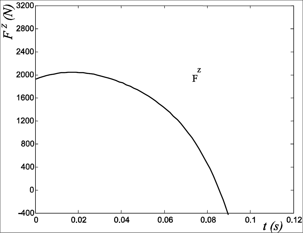
The launching force – the total vertical contact force between the jumper's feet and the ground (in Phase 1).

Figure 6.

Time histories of the main-body (torso) coordinates: x(t), y(t), z(t),θ(t), φ(t), ψ(t).

Figure 7.

Time histories of the joint coordinates: q_j(t), j = 1, … 20.

X(t) = [x(t), y(t), z(t),θ(t), φ(t), ψ(t)] is time history. Figure 7 presents joint trajectories q_j(t), j = 1,…. A selected set of joints is given since not all trajectories are seen as equally interesting. One can notice that from phase to phase different motions are dominant.

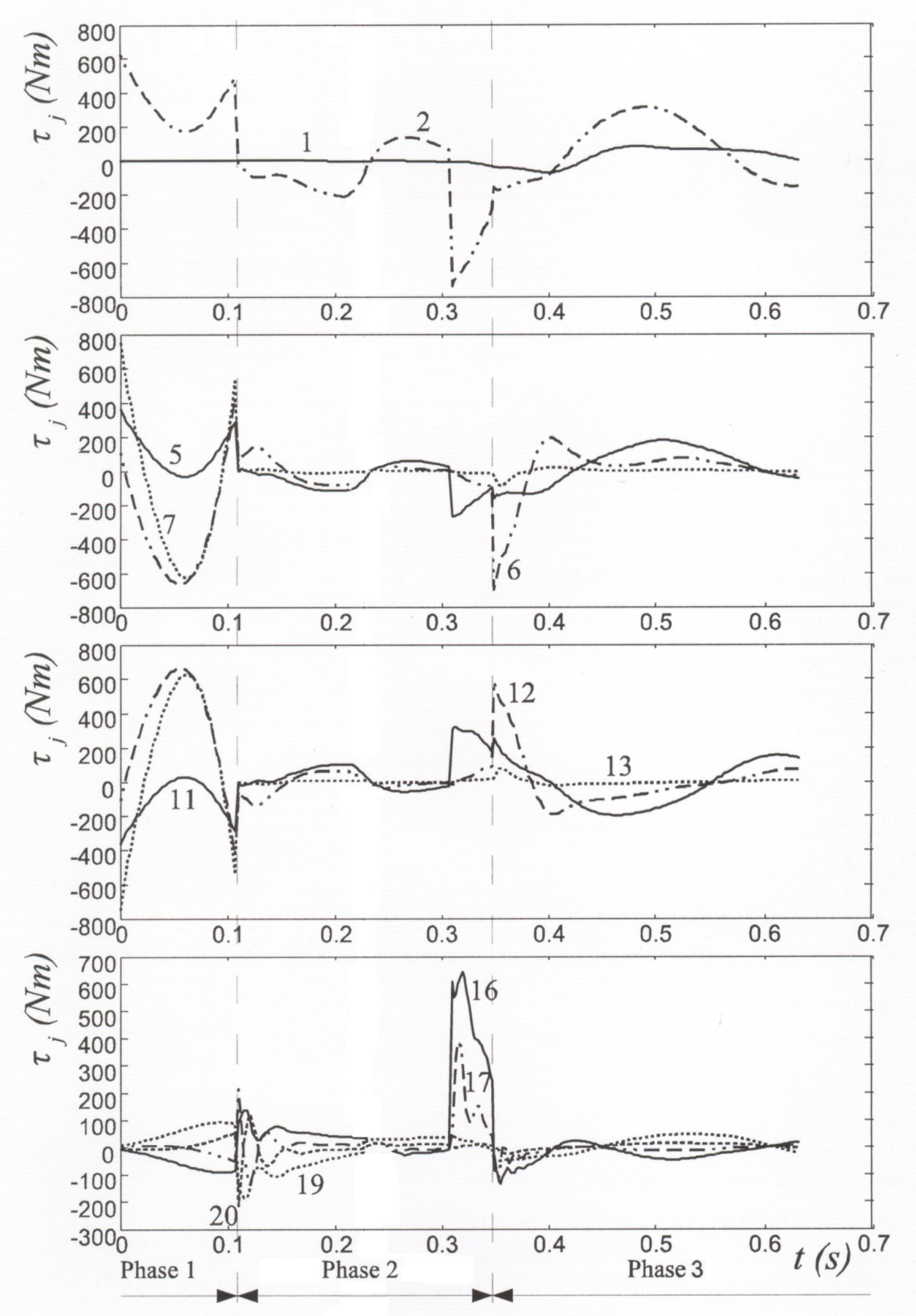
Figure 8 presents the torques generated at the player's joints: τ_j, j = 1,…. A selected set is given. One may see that high torques are present (at relevant joints) during Phase 1 (take off) and Phase 3 take on.

Figure 8.

Time histories of the joint torque: τ_j, J = 1, … 20.

In the swinging phase, it is obvious, as expected, that those high torques are not generated all the time. The arms' torques are not so high, meaning the influence of the arms is not so important during the flight. It is also evident that almost the entire body (the majority of joints) is engaged in this demanding action (jumping).

Regarding the angle of the jumping, the influence of the ankle joint is the most important. The ankle joint has maximum torque all the time, but the duration of the torque determines the angle of the jumping.

Final jump distance depends on several factors. The jump distance achieved affects the movement of the whole body. However, several factors are most important to realize the longest jump. The analyses of the simulated long jump regarding the distance achieved depressed the drive torques at the knees and hips, and made the jump angle. The well-known projectile motion condition gave us the optimal angle of 45%. As already mentioned, the realizations of the jump angle are the most affected by the driving torque at the ankle. Table 2 shows the correlation between achieved distance jump and the intensity of the driving torque at the knees and hips. (The angle of the jump is always 45%).

Table 2.

Knee and hip joint torque influence on the jump length.

Knee joint torque (mN)	Hip joint torque (mN)	Length (m)
200	400	1.05
250	400	1.13
300	400	1.23
200	450	1.35
200	500	1.48
250	450	1.69
250	500	1.83
300	500	1.97

4. Conclusion

This paper proves a general approach to humanoid-robot motion, applicable to any motion task. The extreme complexity of the problem of modelling biological systems stems from the complexity of the mechanical structure and actuation. That is why we started from an approximation – a complex body of a humanoid robot. Since the developed algorithm for the dynamic modelling and the corresponding software do not set limits on the complexity of the humanoid body, we see them as a useful tool for biomechanics as well – a solid approximation of the human body is achieved. At the same time a good foundation is set to develop a truly biological model, as the next research step. In order to avoid an unnecessarily complex problem, we will apply “biological modelling” to key joints only. For a particular action (in every-day life or in sport), key joints will be located and remodelled to agree with their biological structure. New applicability and potentials of the proposed method are demonstrated by simulation of a selected example – the long jump. The simulated motion, including jumping and landing on the feet (after a jump), are presented. Additional analysis is done in the paper regarding the joint torque and joint angle during the jumping. Separate stages of the simulation are defined and explained.

Footnotes

5. Acknowledgments

This work is founded by the Ministry of Education and Science of the Republic of Serbia under the contracts TR-35005 and III-44008. The work is also partially supported by the SNSF Care-robotics project no. IZ74Z0_137361/1.

References

Potkonjak

Vukobratovic

, “A Generalized Approach to Modeling Dynamics of Human and Humanoid Motion”, Intl. Journal of Humanoid Robotics (World Scientific publ.), Vol. 2, No. 1, pp.1–24, 2005.

Vukobratovic

Borovac

, “Zero-Moment Point, Thirty-Five Years of Its Life”, Intern. Journal of Humanoid Robotics, Vol. 1, No 1, pp 157–173, 2004.

Fukuda

Michelini

Potkonjak

Tzafestas

Valavanis

Vukobratovic

, “How Far Away is Artificial Man”, IEEE Robotics and Automation Magazine, March 2001, pp. 66–73, 2001.

Vukobratovic

Potkonjak

Tzafestas

, “Human and Humanoid Dynamics – From the Past to the Future”, Journal of Intelligent and Robotic Systems, Vol. 41 No 1, pp 65–84, 2004.

Vukobratovic

Herr

Borovac

Rakovic

Popovic

Andres

Jovanovic

Potkonjak

, “Biological Principles of Control Selection for a Humanoid Robot's Dynamic Balance preservation” Intern. Journ. of Humanoid Robotics, Vol. 5, No 4, pp 639–678, 2008.

Ken'ichiro

, “Integrated Motion Control for Walking, Jumping and Running on a Small Bipedal Entertainment Robot”, Proceedings of the IEEE International Conference on Robotics, & Automation, 2004, 3189–3194.

Blajer

Czaplicki

, “Modeling and Inverse Simulation of Somersaults on the Trampoline”, Journal of Biomechanics, Vol. 34, 1619–1629, 2001.

Blajer

Czaplicki

, “Contact Modeling and Identification of Planar Somersaults on the Trampoline”, Multibody System Dynamics, Vol. 10, 289–312, 2003.

B. R.

B. J.

Kim

W. K.

, “Impulse Analysis and Its Application to the Dynamic Environment”, Proc of ASME Biennial Mechanism Conf., Montreal, Canada, Sept. 29 – Oct. 2. 2002.

10.

B. R.

B. J.

Sang-Rok

Kim

Y. S.

, “Landing Motion Analysis of Human-Body Model Considering Impact and ZMP condition”, Proceeding of 2004 IEEE/RSJ Intern. Conf. on Intelligent Robots and Systems, Sendai, Japan, 2004, pp1972–1978.

11.

Vukobratovic

Borovac

Potkonjak

Jovanovic

, “Dynamic Balance of Humanoid Systems in Regular and Irregular Gaits: An Expanded Interpretation” Intern. Journ. of Humanoid Robotics, Vol 6. No 1. pp 117–145, 2009.

12.

Potkonjak

Tzafestas

Vukobratovic

Milojevic

Jovanovic

, Human-and-Humanoid Postures Under External Disturbances: Modeling, Simulation, and Robustness. Part 1: Modeling, Journal of Intelligent and Robotic Systems: Theory and Applications, Springer-Verlag Dordrecht, Vol 63, No2. Pp 191–210, 2011.

13.

Potkonjak

Tzafestas

Vukobratovic

Milojevic

Jovanovic

, Human-and-Humanoid Postures Under External Disturbances: Modeling, Simulation, and Robustness. Part 2: Simulation and Robustness, Journal of Intelligent and Robotic Systems: Theory and Applications, Springer-Verlag Dordrecht, Vol 63, No 2. pp 211–231, 2011.