
Abstract
In this paper the kinematic design of a 6-dof parallel robotic manipulator is analysed. Firstly, the condition number of the inverse kinematic jacobian is considered as the objective function, measuring the manipulator's dexterity and a genetic algorithm is used to solve the optimization problem. In a second approach, a neural network model of the analytical objective function is developed and subsequently used as the objective function in the genetic algorithm optimization search process. It is shown that the neuro-genetic algorithm can find close to optimal solutions for maximum dexterity, significantly reducing the computational burden. The sensitivity of the condition number in the robot's workspace is analysed and used to guide the designer in choosing the best structural configuration. Finally, a global optimization problem is also addressed.
1. Introduction
The advantages of manipulators based on parallel design architectures, compared to the serial-based ones, are well recognized and justified by the increasing number of applications which, nowadays, try to explore their inherent low positioning errors and high dynamic performance [1-2]. Among these applications, references can be made to robot manipulators and robotic end-effectors, high speed machine-tools and robotic high-precision tasks, flight simulators and haptic devices [3].
In spite of the inherent general characteristics, the choice of a specific structural configuration and its dimensioning remains a complex problem, as it involves the specification of several design parameters and the consideration of different performance criteria [30]. Optimizing the design to suit a foreseen application remains, therefore, an active area of research.
Optimization based on the manipulator workspace [4-6] is the area upon which most of the research concentrates as it represents one of the main disadvantages, when compared to serial manipulators. In an alternative way, which seeks to explore the parallel manipulator's main advantages, other authors choose to optimize the structural stiffness [7-9]. Several works may also be referred to where the optimization criteria are related with the manipulability, or dexterity, of the manipulator [10-14]. Finally, objective functions based on the manipulator natural frequencies have also been considered [31-32].
Optimization can be a difficult and time consuming task, because of the great number of optimization parameters and the complexity of the objective functions involved. However, optimization procedures based on evolutionary approaches have been proved as an effective solution [15-17, 29].
In this paper the kinematic design of a 6-dof parallel robotic manipulator for maximum dexterity is analysed. The condition number of the inverse kinematic jacobian is used as a measure of dexterity and a Genetic Algorithm (GA) is used to solve the optimization problem. The highly nonlinear nature of the problems involved and the, normally, time consuming optimization algorithms that are used can be naturally approached by artificial Neural Networks (NNs) techniques. In order to explore the advantages of NNs and GAs, a neuro-genetic formulation is developed and tested. In our work we quantify the error of the NN's approximation through testing and validating data sets, and we present a direct comparison of the optima obtained using as the fitness function, either the NN's approximation or the analytical function. This has not been directly addressed in existing research (e.g., [15]).
It is shown that the neuro-genetic algorithm can find close to optimal solutions for maximum dexterity, significantly reducing the computational burden.
Local optimization criteria are especially useful when applied to manipulators with small workspaces, or designed to operate over a small subset of their workspaces. Therefore, a global optimization problem is also addressed and solved.
The paper is organized as follows. Section 2 presents the manipulator architecture and kinematics. In section 3 the optimization problem is formulated and solved using a GA. Section 4 presents a neuro-genetic formulation. In section 5 sensitivity analysis is carried out. In section 6 the global optimization problem is considered and, finally, conclusions are drawn in section 7.
2. Manipulator Architecture and Kinematics
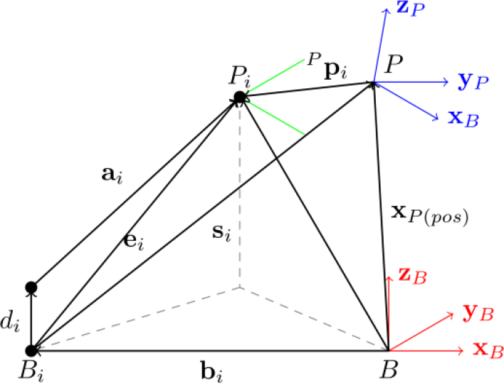
The mechanical architecture of the parallel robot comprises a fixed (base) planar platform and a moving (payload) planar platform, linked together by six independent, identical, open kinematic chains (Figure 1). Each chain comprises two links: the first link (linear actuator) is always normal to the base and has a variable length, l i , with one of its ends fixed to the base and the other one attached, by a universal joint, to the second link; the second link (arm) has a fixed length, L, and is attached to the payload platform by a spherical joint. Points B i and P i are the connecting points to the base and payload platforms. They are located at the vertices of two semi-regular hexagons, inscribed in circumferences of radius r B and r P , that are coplanar with the base and payload platforms (Figure 2).

Schematic representation of the parallel manipulator architecture
For kinematic modelling purposes, a right-handed reference frame {B} is attached to the base. Its origin is located at point B, the centroid of the base. Axis
In a similar way, a right-handed frame {P} is assigned to the payload platform. Its origin is located at point P, the centroid of the payload platform. Axis
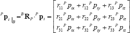
Taking into account the definitions given above, the generalized position of frame {P} relative to frame {B} may be represented by the vector:

where
Vector

Position of the connecting points on the base and payload platform
2.1. Inverse Position Kinematics
The inverse position kinematic model is used to compute the joints positions for a given Cartesian position and orientation. The presented model follows the one proposed in [18].
Taking into account a single kinematic chain, i, vector
p
where
B
Subtracting vectors

Vector
Schematic representation of a kinematic chain
Knowing that the 2-norm of

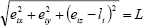
Solving for l i results in

that is, there are two possible solutions for l i . The solutions corresponding to the manipulator having the universal joints below the payload platform spherical joints are always considered:

2.2. Inverse Velocity Kinematics
The inverse velocity kinematics can be represented by the inverse kinematic jacobian, relating the joints velocities to the manipulator Cartesian-space velocities (linear and angular) [18]:

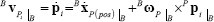
Vector
The velocity of point P
i
is dependent upon the linear and angular velocities of the payload platform. If
where
Squaring both sides of equation (4), the following relation is obtained:

Differentiating equation (10), the following expression results:

where
From equation (11), and taking into account that

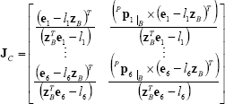
Following this result, the inverse kinematic jacobian may be written (with respect to the base frame) as:
3. Optimization
3.1. Objective Function
Several performance indexes can be formulated based on the manipulator inverse kinematic jacobian [34].
In this work we consider the condition number of the inverse kinematic jacobian matrix,
For example, Salisbury and Craig [20] used the condition number of the jacobian matrix to optimize the finger dimensions of an articulated hand. At the same time they introduced the concept of isotropic configuration, that is, a configuration (mechanical architecture and pose) presenting a condition number equal to one. In an isotropic configuration a manipulator will require equal joint effort to move or produce forces and/or torques in each direction.
Mathematically, the condition number is given by

where
For a 6-dof parallel manipulator, in order to obtain a dimensionally homogeneous jacobian matrix, some kind of normalization procedure has to be used. In this case we use the manipulator payload platform radius, r P , as a characteristic length. In this way, the same ‘cost' will be associated to translational and rotational movements of the payload platform. Using r P as the length unit, the inverse kinematic jacobian results depend upon ten variables, four of them being manipulator kinematic parameters: the position and orientation of the payload platform; the base radius (r B ); the separation angles on the payload platform (φ P ); the separation angles on the base (φ B ); and the arm length (L).
The optimization is done for the manipulator lying in one single configuration (position and orientation); in particular in the centre of the workspace, [0 0 2 0 0 0] T (units in r P and degrees, respectively). Thus, for this pose, the jacobian matrix is a function of the four kinematic parameters.
3.2. Genetic Algorithm-Based Approach
A genetic approach is used to optimize the objective function. The proposed GA uses a real value chromosome given by the four robot kinematic parameters,
The solutions are classified according to the fitness function given by equation (14), in case the solution is admissible, otherwise a large value (1×10²⁰) is assigned.
The global results (Figures 4 and 5) show that there are multiple sets of kinematic parameters that are optimal. Moreover, the algorithm draws a representative solution set of the optimal parameters front. It can be seen, in Figure 5. that the final population set belongs to the best rank (
4. Neuro-Genetic Algorithm-Based Approach
Artificial Neural Networks (NNs) can be considered a problem solving tool with specific characteristics that can be of interest for the development of alternative solutions, to a vast range of problems. In this work we are mainly interested in exploring the well-known capability of NNs to approximate complicated nonlinear functions [27-28], when applied to the objective functions associated with the optimal design of parallel manipulators.
The particular structure of NNs solutions, which is based on the use of a high number of simple processing elements and the respective interconnections, creates a mapping function tool with a high number of adjustable parameters. The process of adjusting these parameters requires the availability of data represented by instances of the problem. Although the design phase can be time consuming and therefore, normally performed in an off-line mode, a trained NN consists of a well-defined and deterministic set of operations which provide an instant solution to a specific instance of the problem, provided it has learned and generalized well.
Our objective was therefore, at this stage, to evaluate the performance of an NN developed to map the condition number function of the inverse jacobian, κ, of equation (14).

Simulation results: optimal sets of kinematic parameters. The marked points are used in in the sensitivity analysis (section 5). The observed small differences in the numerical values are due to the finite resolution of the mesh.
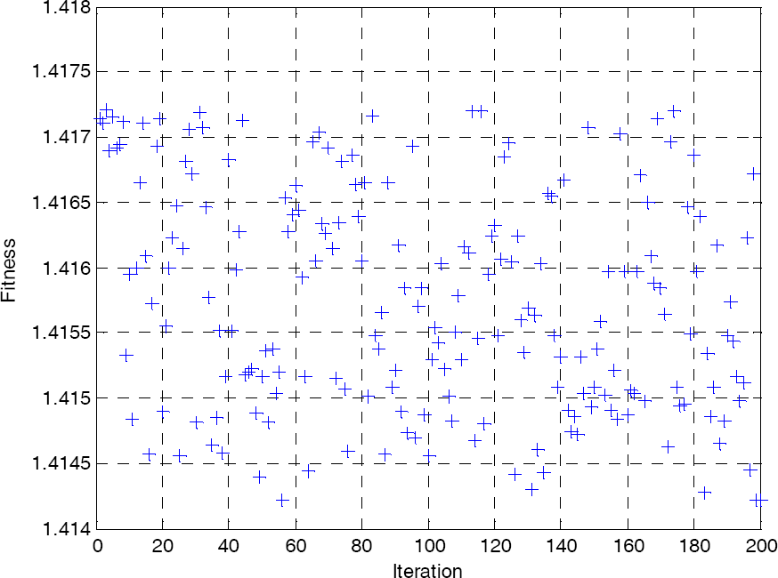
Simulation results: fitness function values for 200 sets of optimal solutions
4.1. Development of an Artificial Neural Network Mapping of the Objective Function
The process of designing an NN solution to a specific problem is mainly guided by trial and experimentation, due to the lack of explicit and proven methods that can be used to choose and set the various parameters involved in the NN design process.
Among the different structures and types of NN available, the experiments were done using classical multilayer feedforward architecture. However, instead of using the standard backpropagation learning algorithm, training was performed using the Levenberg-Marquardt (LM) algorithm, which represents a faster alternative and also benefits from an efficient implementation in Matlab® software.
The representation of the problem in this multilayer NN structure was to provide at the input layer the four kinematic parameters (r B , φ P , φ B , L) and to produce the condition number of the inverse jacobian (κ) at the output layer (Figure 6). The number of intermediate layers, i.e., hidden layers, and the respective number of hidden elements were established based on multiple experiments with various combinations. From these experiments, networks with one hidden layer and three different numbers of hidden elements (25, 50, and 100) were selected.

Feedforward NN elements (4 Inputs, 1 Hidden layer, 1 Output)
The data used to develop the networks was obtained by generating random values for each of the four arguments and eliminating the impossible combinations (i.e., negative κ values). The cases generated were split into training (70%), validating (15%) and testing (15%) data sets. As can be observed in Figure 7, the three sets have similar distributions. Furthermore, the cases with lowest κ values (i.e., below 2.0) are very few (five in total) and most cases are also well below the maximum values obtained. The minimum and maximum values for these sets are: TRA(1.4656; 12.0140), VAL(1.4170; 10.7360) e TES(1.4545; 10.2760).
The training and testing steps performed in each experiment followed common procedures, such as normalizing the data cases used, starting the learning process from different random initial states and observing performance along the training iterations. The performance measure used was the mean square error function (mse), calculated for each of the three data sets, as can be observed in Figure 8. The learning process was controlled based on the behaviour of the mse function, i.e., the number of successive increases, on the validation set.
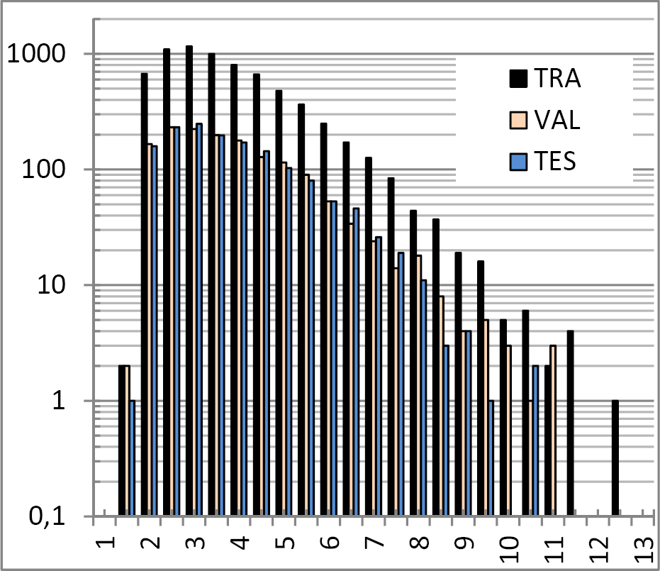
Histogram representation of the κ value's distribution for the three data sets: training (TRA), 6999 cases, validating (VAL), 1500 cases and testing (TES), 1500 cases
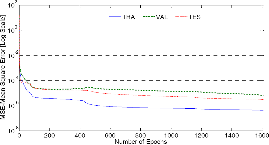
Performance measure (mse) evolution during the training iterations (epochs): training (TRA), validating (VAL) and testing (TES) data sets
Subsequent to the learning process, the performance of the trained network was analysed, after reverting normalization in the data sets, through the maximum and minimum error values and the root mean square error (rmse) (Table 1). Considering the range of values of the objective function included in the data sets [1.4170, 12.0140], the results obtained with mapping the objective function using NNs show that a good approximation is possible in average terms (i.e.,
Having developed an NN approximation of the condition number of the inverse jacobian (κ), the objective was to evaluate whether the NN approximation could be used, as the fitness function, in a search for minimum values through GAs. In this way it will open up an opportunity to use NNs in the optimal design of parallel manipulators.
Performance of a neural network with 50 hidden elements, relative to desired output (i.e., Target-NN output), after reversing normalization: square root of mean square error (

The experiments performed in the minimization search use various NN approximations and also the analytical function. In each search, the 200 best cases found were considered for comparison. Figure 9 illustrates the results obtained using NNs with a different number of hidden elements (25, 50, and 100) and with the analytical function. It can be observed that in general the GA process using NNs converged to minimum values of the approximated function. However, these values were well above the minimum values, i.e., [1.41 to 1.42], obtained when using the analytical function. Furthermore, the smaller the network sizes, in general, the approximated values are reduced to a minimum.
The higher minimum values of the NNs' approximations can be explained considering the distribution of the data sets used to develop the NNs (Figure 7). Only five cases (two in the training set, two in the validating set and one in the testing set) were cases with a k value below 2.0. This also supports the common belief that NNs are better interpolators than as extrapolating.
Comparing the series of minimum values obtained with the different NNs, the NNs with a lower number of elements in the hidden layer converged to lower values in the minimization process. This also seems to agree with the belief that smaller networks will tend to generalize better than larger networks. To complement this analysis, a comparison of the approximation values provided by each network with the real values can be observed in Figure 10 (50 hidden elements network) and Figure 11 (25 hidden elements network). It can be observed that the smaller size NN, provides lower approximated k values (Figure 9), which also represent lower real values (Figure 11). However, when compared to a larger size network, in Figures 9 and 11, they are more dispersed. In addition, they include more cases where the NN's approximation is below the real value.
From these experiments it can be said that an approximation to complex functions by an NN can be used in the process of finding optimum solutions for the design of parallel manipulators. In spite of their inherent limitations to extrapolate well to the minimum values of a function, they converge to close to minimum values, which in a multi-criteria optimization problem may be less significant. Furthermore, the use of the GA-NN based approach was able to reduce the search time by 30% to 50%, compared to the use of a GA analytical function. The time to develop the NN is not included, but in a case where the analytical function is also not available, such for example, on a multi-criteria optimization case, this as well, adds favourably to the advantages of NN-based solutions.

Values of the objective function (κ) for each of the 200 considered best cases: GA-Analytical Func., GA-NN25 Hid. El., GA-NN50 Hid. El., GA-NN100 Hid. El.
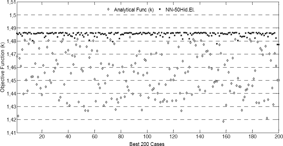
Values of the objective function (κ) for each of the 200 considered best cases using 50 Hidden Ele. NN: values of the analytical function and values of the NN approximation.

Values of the objective function (κ) for each of the 200 considered best cases using the 25 Hidden Ele. NN: values of the analytical function and values of the NN approximation.
5. Sensitivity Analysis
As seen in the previous sections, the optimization algorithm draws a representative solution set of the front of optimal parameters. As the robot designer has to choose one optimal solution among a large set of candidates, additional information must be provided to support her/his job.
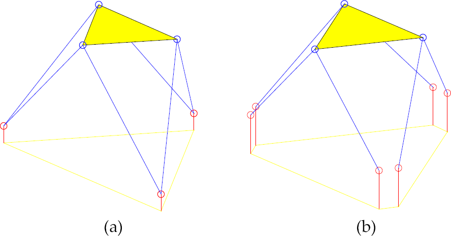
Schematic representation of the parallel manipulator for two optimal solutions (a) configuration 1; (b) configuration 2
In this section a sensitivity analysis is presented, showing how the analytical objective function, κ, evolves inside a given workspace. Two representative, and almost opposite, optimal solutions are considered. Configuration 1 (Figure12a) corresponding to the set of parameters [r B φ P φ B L] T = [2.0113r P 0° 0° 2.4643r P ] T , which means a 3-3 type architecture (triangular base and payload platforms) with a large L and configuration 2, described by the kinematic parameters [1.7321r P 0° 5.2635° 2.0000r P ] T , corresponding to a 6-3 type architecture (hexagonal base and triangular payload platform) with a shorter L (Figure 12 b). Usually, larger values of L are desirable in order to have larger workspaces.
Figures 13 to 16 show the variation of κ in a given manipulator workspace. The workspace is described by a mesh of points on the surface of a sphere with radius 0.3 r P . The centre of the mobile platform is then positioned in all points of the mesh and rotated by an angle between −30° and 30° in any direction. At each point of the discretized workspace the condition number, κ, was evaluated. As can be seen in the figures 13 to 16, κ, is minimum at the centre of the workspace, getting higher as the distance to the centre increases. Moreover, it can be noticed that configuration 2 is more sensitive to the distance than configuration 1, because κ increases faster.

Variation of κ with respect to x and y (a) for configuration 1; (b) for configuration 2
On the other hand, for the workspace mentioned above, the maximum displacement of the actuators and the extreme values of κ and singular values were analysed. Table 2 shows the main results.
Maximum actuators displacement and extreme values of κ and singular values
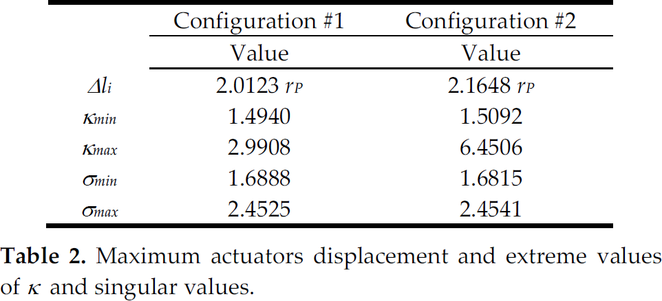
Figures 18 and 19 represent the manipulator poses corresponding to the parameters shown in Table 2, for the two considered configurations.

Variation of κ with respect to ψ and θ (a) for configuration 1; (b) for configuration 2
According to the sensitivity analysis, it might be concluded that configuration 1 will correspond to the best performance.
A triangular payload platform results in double spherical joints connecting the kinematic chains to that platform. As the mechanical solution for this is well known, the main disadvantage is the propensity to increase kinematic chain interference, because the physical dimensions of the links are usually bigger.
A triangular base platform results in three pairs of coincident actuators, leading to an even more complicated mechanical design. Therefore, a trade-off must be taken into account between better performance and harder mechanical design.

Variation of κ with respect to ψ and φ (a) for configuration 1; (b) for configuration 2
Similar results were obtained when the sensitivity analysis was carried out using the NN approximated objective function. Figure 17 illustrates one representative case of an NN solution (green surface) and a comparable analytical solution (red surface) in terms of dexterous workspace; a very similar behaviour can be observed. The NN solution is only clearly over the analytical solution farther away from the centre of the workspace. This goes in line with the GA-NN solutions, in general providing slightly worst solutions, but faster computational times.

Variation of κ with respect to θ and φ (a) for configuration 1; (b) for configuration 2

Variation of κ with respect to x and y, for configuration 1. The red surface is the result obtained using the analytical objective function; the green one corresponds to the function given by the NN.

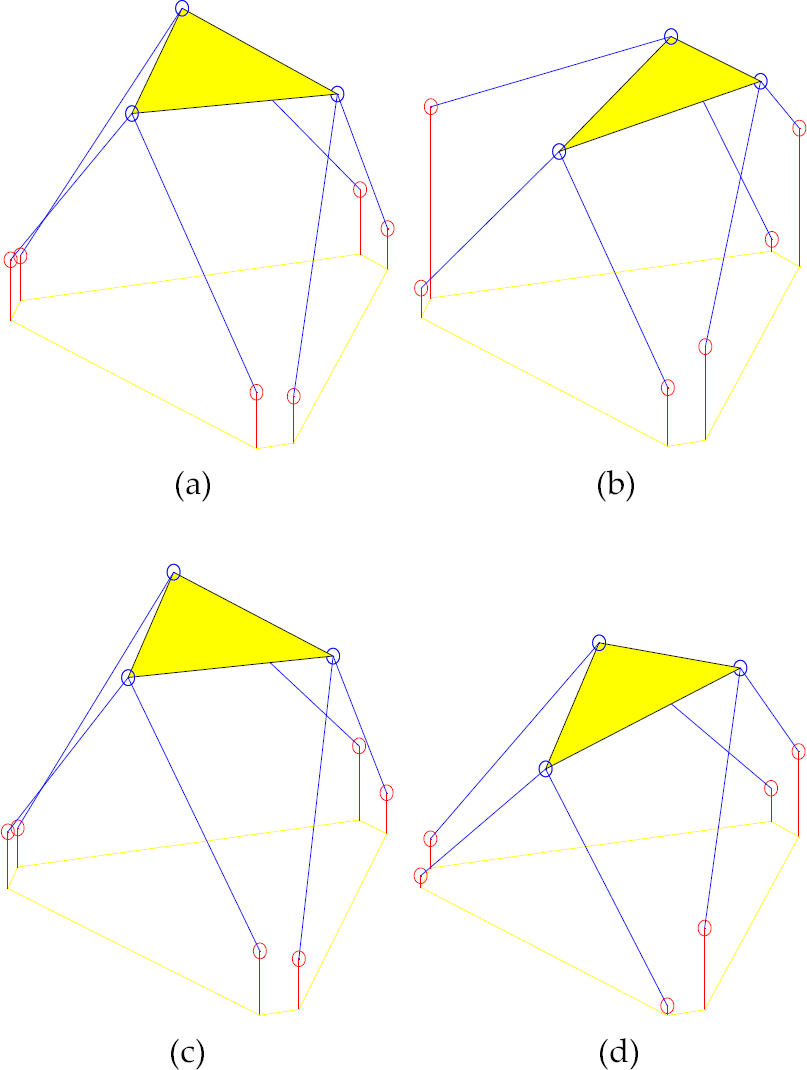
Manipulator poses corresponding extreme values of κ and singular values for configuration 1 (a) σ min ; (b) σ max ; (c) κ min ; (d) κ max.
Manipulator poses corresponding to extreme values of and singular values for configuration 2 (a) σmin; (b) σmax; (c) κmin; (d) κmax
Manipulator poses corresponding to extreme values of κ and singular values for configuration 2 (a) σmin; (b) σmax; (c) κmin; (d) κmax.
6. Global Optimization
In this section the previous approach is generalized and used in a global optimization problem. The objective function is the global index given by equation (15).

where the reciprocal of the condition number is evaluated in the manipulator workspace, W. The reciprocal of the condition number is used because it is numerically better behaved. Equation (15) is approximated by

where the value of χ is calculated after discretization of the manipulator workspace and computation of 1/κ at each of the n points of the resulting mesh.
For simulation, to reduce the computational load, we consider the particular case of a manipulator having a triangular payload platform, φ P = 0. The workspace is the hyper-volume defined by −0.4 ≤ x P , y P , z P ≤ 0.4 for translations (units in r P ), and −25° ≤ ψ P , θ P , φ P ≤ 25° for rotations. The allowed variation of the manipulator parameters is 1.0 ≤ r B ≤ 2.5 r P , 0° ≤ φ B ≤ 25° and 3.0 ≤ L ≤ 4.5 r P .
Figure 20 illustrates the evolution of the global index versus the manipulator parameters. It can be seen, for a given solution of the optimal set, [r B φ B L] = [2.5 0 3.6], that the global index degrades considerably as a consequence of optimal parameters detuning.
7. Conclusions
In this paper the kinematic design of a 6-dof parallel robotic manipulator for maximum dexterity was analysed. First, a GA was utilized to solve the optimization problem. Afterwards, a neuro-genetic formulation was developed and tested. The GA converged to optimal solutions characterized by multiple sets of optimal kinematic parameters. Moreover, the GA provides a representative solution set of the parameters front. NNs were used to map nonlinear objective functions associated with the design of parallel manipulators. The performance obtained showed they can be used as the fitness function in a GA minimization process, reducing the computational time. Since the optimization algorithm draws several optimal solutions, a sensitivity analysis was performed in order to guide the robot designer to select the best structural configuration. Although the final solutions have all the same objective value, κ, the analysis reveals that some architectures might be preferred. The approach can be easy generalized and used in a global optimization problem.

Global index vs. (a) (L, rB), φB = 0; (b) (L, φB), rB = 2.5; (c) (rB, φB), L = 3.6