Sage Journals: Discover world-class research

Abstract

One important issue in a machining robotic cell is the location of the workpiece with respect to the robot. The feasibility of the task, the quality of the final work and the energy consumption, just to mention a few, are all dependent upon it. This can be formulated as an optimization problem where the objective functions are chosen in order to meet desired performance criteria. Typically, the complexity of the problems and the large number of optimization parameters that, usually, are involved, make the genetic algorithms an appropriate tool in this context. In this paper, two optimization problems are formulated: firstly, the power consumed by the manipulator is considered and the problem is solved using a single-objective genetic algorithm; then the stiffness of the manipulator is also included and the respective optimization problem is solved using a multi-objective genetic algorithm. Simulation results are presented for a parallel manipulator robotic cell.

Keywords

Robotics Parallel Manipulator Dynamics Robot Machining Genetic Algorithm

1. Introduction

Robots have been widely used in industry to carry out several tasks, like welding, painting, assembly, pick and place, and palletizing, just to mention a few [1, 2]. On the other hand, CNC machine tools have been exclusively devoted to high precision manufacturing.

Typically, robots have large workspaces and good dexterity, and have become more and more accurate due to important advances in electronics, informatics, control and mechanical design. Recently, robots started to be regarded as low-cost alternatives to machine tools [3-12]. In fact, machining of soft materials (such as polymers and composites), machining of large wood or stone workpieces, and end-machining of middle tolerance parts, are examples of tasks that can be carried out at lower costs using robots. Pre-machining of foundry parts and rapid prototyping are two additional areas where robots can also be used instead of machine tools [8, 9].

Several recent works have dealt with robotic machining. In [13], for example, a method for high-precision drilling using an industrial robot was presented. The robot is equipped with a six degrees-of-freedom (dof) force/torque sensor and an active force control strategy was designed to regulate the interaction forces between the robot and the workpiece. In [14] the authors use a milling serial robot, proposing a method to find the appropriate location of the robot with respect to the workpiece, in order to optimize the manipulability and joint torques. A similar problem was addressed in [15]. In that work, an optimization algorithm was used to find the appropriate position and joint angles of a serial robot, avoiding singular configurations. In [16] the vibration response of a robotic machining system was studied and a method based on the variation of the speed of the spindle was introduced to minimize vibration. Robotic machining has also been used in non-industrial environments. As an example, [17] deals with machining of bones in orthopaedic surgery.

An important issue in a machining robotic cell is the positioning of the workpiece with respect to the robot. The best position depends on the task or, more precisely, on the trajectory and on the forces that the robot exerts on the workpiece. This problem can be formulated as an optimization problem where the objective functions are chosen in order to meet specific performance criteria. Optimization can be a difficult and time-consuming task, because of the great number of optimization parameters and the complexity of the objective functions that usually are involved. The optimization procedures based on evolutionary approaches have been proved as an effective way out [18].

Robot trajectory planning and optimal design are typical optimization problems that are often solved using this class of algorithms. In [19], for example, a Genetic Algorithm (GA)–simplex hybrid optimization method is used to synthesise a spatial 3-RPS parallel manipulator. The method firstly carries out a global search for the solution using a GA and then applies the simplex method for a final local search. In [18] the kinematic design of a 6-dof parallel robotic manipulator for maximum dexterity is analysed. A GA and a neuro-genetic formulation are proposed to solve the optimization problem. In [20] a multi-objective evolutionary algorithm is proposed for optimal trajectory planning of a parallel manipulator. Minimum time and energy are the adopted performance criteria. A similar problem was addressed by [21] where a hybrid strategy was used for time and energy efficient trajectory planning of parallel platform manipulators.

In this paper the optimal location of the workpiece with respect to the robot, in a machining robotic cell is analysed. We formulate the problem supposing that the robot exerts a certain contact force and executes a specific trajectory on the surface of the workpiece. The force and the trajectory might have been computed by a higher-level intelligent layer, taking into account the specific issues related to the machining processes. This topic is not covered in this work.

The adopted robot possesses a parallel structure. Parallel manipulators have considerable advantages over the serial-based ones, such as higher precision and stiffness, and better dynamic characteristics [22, 23].

Two optimization problems are formulated: firstly, the power consumed by the manipulator is considered and the problem is solved using a single-objective GA; then the stiffness of the manipulator is also taken into account and the respective optimization problem is solved using a multi-objective GA.

Bearing these ideas in mind, the paper is organized as follows. Section 2 deals with the manipulator and the respective kinematic model. In section 3 the manipulator dynamic model is presented. Since the manipulator dynamics typically involves demanding calculations, a simple and efficient model is proposed. Section 4 presents the objective functions. In section 5, the optimization problems are formulated and solved using GAs. Finally, conclusions are drawn in section 6.

2. Robot Kinematics

A 6-dof variant of the well-known Stewart platform manipulator [22] is considered. Its mechanical structure comprises a fixed (base) platform and a moving (payload) platform, linked together by six independent, identical, open kinematic chains (Figure 1).

Figure 1.

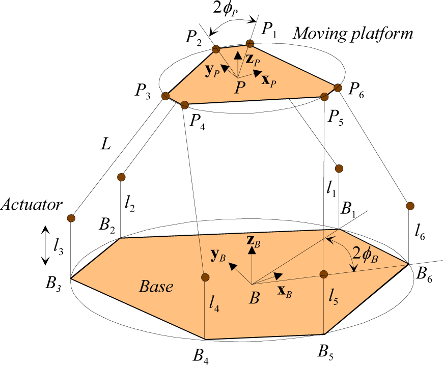
Schematic representation of the kinematic structure of the parallel manipulator

Each chain comprises two links: the first link (linear actuator) is always normal to the base and has a variable length, l_i (i = 1, …, 6) with one of its ends fixed to the base and the other one attached, by a universal joint, to the second link; the second link (arm) has a fixed length, L, and is attached to the payload platform by a spherical joint. Points B_i and P_i are the connecting points to the base and payload platforms. They are located at the vertices of two semi-regular hexagons, inscribed in circumferences of radius r_B and r_P, that are coplanar with the base and payload platforms. The separation angles between points B₁ and B₆, B₂ and B₃, and B₄ and B₅ are denoted by 2φ_B. In a similar way, the separation angles between points P₁ and P₂, P₃ and P₄, and P₅ and P₆ are denoted by 2φ_P.

For modelling purposes, two frames, {P} and {B}, are attached to the centre of mass of the moving and base platforms, respectively, the generalized position (pose) of frame {P} relative to frame {B} may be represented by the vector:

^{B} x_{P |_{B | E}} = \begin{matrix} [^{B} x_{P (p o s) |_{B}}^{T} & ^{B} x_{P (o) |_{E}}^{T} \end{matrix}]^{T}

(1)

where $^{B} x_{P (p o s) |_{B}}^{} = {[\begin{matrix} x_{P} & y_{P} & z_{P} \end{matrix}]}^{T}$ is the position of the origin of frame {P} relative to frame {B}, and $^{B} x_{P (o) |_{E}}^{} = {[\begin{matrix} ψ_{P} & θ_{P} & φ_{P} \end{matrix}]}^{T}$ defines an Euler angles system representing the orientation of frame {P} relative to {B}. The rotation matrix is given by:

^{B} R_{P} = [\begin{matrix} C ψ_{P} C θ_{P} & C ψ_{P} S θ_{P} S φ_{P} - S ψ_{P} C φ_{P} & C ψ_{P} S θ_{P} C φ_{P} + S ψ_{P} S φ_{P} \\ S ψ_{P} C θ_{P} & S ψ_{P} S θ_{P} S φ_{P} + C ψ_{P} C φ_{P} & S ψ_{P} S θ_{P} C φ_{P} - C ψ_{P} S φ_{P} \\ - S θ_{P} & C θ_{P} S φ_{P} & C θ_{P} C φ_{P} \end{matrix}]

(2)

S() and C() correspond to the sine and cosine functions, respectively.

The inverse velocity kinematics can be represented by the inverse kinematic jacobian, J_C, relating the velocities of the joints and the velocities (linear and angular) of the payload platform:

{\dot{I} = J}_{c} \cdot^{B} {\dot{x}}_{P |_{B}}

(3)

Vector $\dot{l} = \begin{matrix} [{\dot{l}}_{1} & {\dot{l}}_{2} & \dots & {\dot{l}}_{6} \end{matrix}]^{T}$ represents the joints velocities, and vector $^{B} \dot{x}_{P |_{B}} = {\begin{matrix} [^{B} \dot{x}_{P (p o s) |_{B}}^{T} & ^{B} ω_{P |_{B}}^{T}] \end{matrix}}^{T}$ represents the Cartesian-space velocities.

The inverse jacobian matrix is given by equation (4), which can be computed using vector algebra.

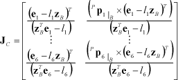
J_{C} = [\begin{matrix} \frac{{(e_{1} - l_{1} z_{B})}^{T}}{(z_{B}^{T} e_{1} - l_{1})} & \frac{(^{P} p_{1 |_{B}} \times {(e_{1} - l_{1} z_{B})}^{T})}{(z_{B}^{T} e_{1} - l_{1})} \\ ⋮ & ⋮ \\ \frac{{(e_{6} - l_{6} z_{B})}^{T}}{(z_{B}^{T} e_{6} - l_{6})} & \frac{(^{P} p_{6 |_{B}} \times {(e_{6} - l_{6} z_{B})}^{T})}{(z_{B}^{T} e_{6} - l_{6})} \end{matrix}]

(4)

All vectors are obtained analyzing a kinematic chain of the parallel manipulator (Figure 2). Vector e_i is given by

e_{i} =^{B} x_{P (p o s) |_{B}} - b_{i} +^{P} p_{i |_{B}}

(5)

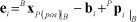
where b_i represents the position of point B_i and $^{P} p_{i |_{B}}$ is the position of point P_i, on the mobile platform, expressed in the base frame. The scalar l_i is the displacement of each actuator, given by equation (6), which represents the inverse position kinematics.

l_{i} = e_{i z} + \sqrt{L^{2} - e_{i x}^{2} - e_{i y}^{2}}

(6)

As the angular velocity and the time derivatives of the Euler angles are related by

^{B} ω_{P |_{B}} = J_{A} \cdot^{B} \dot{x}_{P (o) |_{E}}

(7)

the following equation can be written:

\dot{l} = J_{E} \cdot^{B} \dot{x}_{P_{| E}}

(8)

where J_E is the Euler angles inverse jacobian matrix, and J_A is given by equation (9).

J_{A} = [\begin{matrix} 0 & - S ψ_{P} & C θ_{P} C ψ_{P} \\ 0 & C ψ_{P} & C θ_{P} S ψ_{P} \\ 1 & 0 & - S θ_{P} \end{matrix}]

(9)

Figure 2.

Schematic representation of a kinematic chain

3. Robot Dynamics

Robot dynamics can be computed through the well known Lagrange Equation (LE). Expressing LE as a function of the moving platform generalized position, $^{B} x_{P |_{B | E}}$ , results in:

\frac{d}{d t} (\frac{\partial K (^{B} x_{P |_{B | E}},^{B} {\dot{x}}_{P |_{B | E}})}{\partial^{B} {\dot{x}}_{P |_{B | E}}}) - \frac{\partial K (^{B} x_{P |_{B | E}},^{B} {\dot{x}}_{P |_{B | E}})}{\partial^{B} x_{P |_{B | E}}} + \frac{\partial P (^{B} x_{P |_{B | E}})}{\partial^{B} x_{P |_{B | E}}} =^{P} f_{|_{B | E}}

(10)

where K and P are the total kinetic and potential energies, and $^{P} f_{|_{B | E}}$ represents the generalized force acting on the centre of mass of the moving platform. This vector may be written as:

^{P} f_{|_{B | E}} = {\begin{matrix} [^{P} F_{|_{B}}^{T} & ^{P} M_{|_{E}}^{T}] \end{matrix}}^{T}

(11)

Vector $^{P} F_{|_{B}}$ represents the total force acting on the centre of mass of the moving platform, expressed in the base frame, {B}, and vector $^{P} M_{|_{E}}$ represents the total momentum acting on the moving platform, expressed using the Euler angles system. As the vector $^{P} M_{|_{E}}$ doesn't have a clear physical meaning, the vector

^{P} M_{|_{B}}^{} = J_{A}^{- T} \cdot^{P} M_{|_{E}}^{}

(12)

can be defined, which represents the momentum vector applied on the mobile platform and expressed in the base frame {B}. The actuators forces, τ, may be computed using the statics equation:

τ = J_{E}^{- T} \cdot^{P} f_{|_{B | E}}

(13)

3.1. Manipulator Kinetic Energy

The total kinetic energy, K, can be computed as the sum of the kinetic energies of all rigid bodies: the moving platform, the 6 actuators and the 6 fixed-length links:

K = K_{P} + \sum_{i = 1}^{6} K_{A_{i}} + \sum_{i = 1}^{6} K_{L_{i}}

(14)

where K_P, $K_{A_{i}}$ and $K_{L_{i}}$ represent the moving platform, each actuator, and the fixed-length link kinetic energies, respectively.

3.1.1. Moving Platform Kinetic Energy

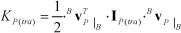
The moving platform kinetic energy is the sum of two components, as shown in equation (15), the translational kinetic energy, K_P(tra), and the rotational kinetic energy, K_P(rot).

K_{P} = K_{P (t r a)} + K_{P (r o t)}

(15)

The translational kinetic energy may be easily computed using the following equation:

K_{P (t r a)} = \frac{1}{2} \cdot^{B} v_{P |_{B}}^{T} \cdot I_{P (t r a)} \cdot^{B} v_{P |_{B}}

(16)

where I_P(tra) is the translational inertia matrix of the moving platform and m_P is its mass:

I_{P (t r a)} = diag ([\begin{matrix} m_{P} & m_{P} & m_{P} \end{matrix}])

(17)

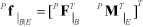
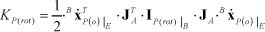
The rotational kinetic energy may be computed using equation (18):

K_{P (r o t)} = \frac{1}{2} \cdot^{B} ω_{P |_{B}}^{T} \cdot I_{P (r o t) |_{B}} \cdot^{B} ω_{P |_{B}}^{}

(18)

Matrix $I_{P (r o t) |_{B}}$ represents the rotational inertia matrix, expressed in the base frame {B}. This matrix can be written as a function of the rotational inertia matrix expressed in the moving platform frame {P}, $I_{P (r o t) |_{P}}$ :

I_{P (r o t) |_{B}} =^{B} R_{P} \cdot I_{P (r o t) |_{P}} \cdot^{B} R_{P}^{T}

(19)

I_{P (r o t) |_{P}} = diag ({[\begin{matrix} I_{P_{x x}} & I_{P_{y y}} & I_{P_{z z}} \end{matrix}]}^{^{}})

(20)

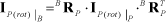
Using equations (7) and (19) we have:

K_{P (r o t)} = \frac{1}{2} \cdot^{B} {\dot{x}}_{P (0)}^{T} |_{E} \cdot J_{A}^{T} \cdot I_{P (r o t) |_{B}} \cdot J_{A} \cdot^{B} {\dot{x}}_{P (0) |_{E}}

(21)

3.1.2. Actuators Kinetic Energy

As the actuators can only move perpendicularly to the base, their angular velocity relative to frame {B} is always zero. If the actuators are assumed to be equal, and the centre of mass of each actuator, cm_A, is located at a fixed distance, a_cm, from the actuator to the fixed-length link connecting point (Figure 3), the position of the centre of mass relative to frame {B} is:

^{B} p_{A_{i} |_{B}} = b_{i} + (l_{i} - a_{c m}) \cdot z_{B}

(22)

The linear velocity of the centre of mass of the actuator, $^{B} \dot{p}_{A_{i} |_{B}}$ , relative to {B} and expressed in the same frame may be computed from the time derivative of the previous equation:

^{B} {\dot{p}}_{A_{i} |_{B}} = {\dot{l}}_{i} \cdot z_{B}

(23)

Figure 3.

Actuator centre of mass position

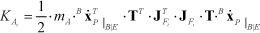
The kinetic energy of each actuator is

K_{A_{i}} = \frac{1}{2} \cdot m_{A} \cdot^{B} {\dot{p}}_{A_{i} |_{B}}^{T} \cdot^{B} {\dot{p}}_{A_{i} |_{B}} = \frac{1}{2} \cdot m_{A} \cdot l_{i}^{2}

(24)

where m_A is the actuator mass. Thus, using the velocity kinematics, we may write:

{\dot{l}}_{i} = J_{F_{i}} \cdot [\begin{matrix} ^{B} v_{P |_{B}} \\ ^{B} ω_{P |_{B}} \end{matrix}] = J_{F_{i}} \cdot T \cdot^{B} {\dot{x}}_{_{P |_{B | E}}}

(25)

where $J_{F_{i}}$ represents the line i of the jacobian, J_C, and

T = diag ([\begin{matrix} I & J_{A} \end{matrix}])

(26)

Equation (24) may be rewritten in the following final form:

K_{A_{i}} = \frac{1}{2} \cdot m_{A} \cdot^{B} {\dot{x}}_{p |_{B | E}}^{T} \cdot T^{T} \cdot J_{F_{i}}^{T} \cdot J_{F_{i}} \cdot T \cdot^{B} {\dot{x}}_{P |_{B | E}}

(27)

3.1.3. Fixed-length Links Kinetic Energy

Computation of the fixed-length links dynamic contributions requires high computational effort. To simplify the problem, each fixed-length link is modelled as a zero-mass virtual link connecting two point masses located at its ends. This is a reasonable simplification as the fixed-length links are connected to the moving platform and to the actuators by universal joints. We consider that the fixed-length link mass, m_L, is the sum of two components, m_L1 is a point mass located at the connection point between the moving platform and the fixed-length link, and m_L2 is a point mass located at the connection point between the actuator and the fixed-length link: $m_{L} = m_{L 1} + m_{L 2}$ . It should be noted this is equivalent to consider m_L1 and m_L2 as part of the moving platform and actuators, respectively. Then, the fixed-length links don't need to be modelled as independent rigid bodies, and their masses are distributed between the moving platform and the actuators:

m_{A (n e w)} = m_{A} + m_{L 2}

(28)

m_{P (n e w)} = m_{P} + 6 m_{L 1}

(29)

I_{P (r o t) (n e w) |_{P}} = I_{P (r o t) |_{P}} + diag ({[\begin{matrix} I_{x x} & I_{y y} & I_{z z} \end{matrix}]}^{^{}})

(30)

I_{x x} = 2 m_{L 1} r_{P}^{2} [\sin^{2} (\frac{π}{3} - ϕ_{P}) + \sin^{2} (\frac{π}{3} + ϕ_{P}) + \sin^{2} (ϕ_{P})]

(31)

I_{y y} = 2 m_{L 1} r_{P}^{2} [\cos^{2} (\frac{π}{3} - ϕ_{P}) + \cos^{2} (\frac{π}{3} + ϕ_{P}) + \cos^{2} (ϕ_{P})]

(32)

I_{z z} = 6 m_{L 1} r_{P}^{2}

(33)

4. Objective Functions

Several objective functions may be adopted, depending on the robotic cell and the task to be carried out.

Firstly, the mechanical power dissipated by the robot actuators, P_act, along the discretized trajectory is analysed. Mathematically, the mechanical power is given by (34):

P_{a c t} = \sqrt{\sum_{k = 1}^{K} \sum_{i = 1}^{6} {[τ_{i} (k) \cdot {\dot{l}}_{i} (k)]}^{2}}

(34)

where K is the total number of points, that depends on the discretizing period and the trajectory time length. This function should be minimized.

Another important objective in robotic machining is the maximization of the stiffness of the manipulator along its trajectory. The stiffness may be regarded as a measure of the ability of the robot to resist deformation due to the action of external forces. This characteristic is especially important in applications that involve interaction between the manipulator and the environment, affecting the precision of the robot and the quality of the executed task. On the other hand, higher stiffness typically allows higher velocities and lower vibrations of the mechanical structure. At any pose the stiffness of the robot can be characterized by the stiffness matrix, which relates the Cartesian forces and torques, applied on the end-effector, to the corresponding linear and angular displacements.

Giving the equation (3) we may write

Δ I \approx J_{c} \cdot^{B} Δ x_{P |_{B}}

(35)

where $Δ l$ represents an infinitesimal displacement of the actuators and $^{B} Δ x_{P |_{B}}$ represents the corresponding displacement in the Cartesian space. Moreover, using the duality between differential kinematics and static results in

^{P} f_{|_{B}} = J_{C}^{T} \cdot τ

(36)

where $^{P} f_{|_{B}}$ represents the force and torque applied on the payload platform, and τ represents the forces on the actuators.

Adopting a finite stiffness in each actuator, given by k_i, then the corresponding force, τ_i, and displacement, Δl_i, are related by $τ_{i} = k_{i} \cdot Δ l_{i}$ , according to Hooke's law. Considering that all actuators are identical, the following equation can be written:

τ = K \cdot Δ l

(37)

with $K = diag ({[\begin{matrix} k_{1} & k_{2} & \dots & k_{6} \end{matrix}]}^{T})$ representing the stiffness matrix expressed in the space of the actuators.

Using equations (35) to (37), results in:

^{P} f_{|_{B}} = J_{C}^{T} \cdot K \cdot J_{C}^{} \cdot Δ^{B} x_{P |_{B}}

(38)

where $K_{|_{B}} = J_{C}^{T} \cdot K \cdot J_{C}^{}$ is the Cartesian-space stiffness matrix.

In the particular case of identical actuators, then k_i = k and

^{P} f_{|_{B}} = k \cdot J_{C}^{T} \cdot J_{C}^{} \cdot Δ^{B} x_{P |_{B}}

(39)

K_{|_{B}} = k \cdot J_{C}^{T} \cdot J_{C}^{}

(40)

Mathematically, the objective function that is adopted to quantify the stiffness of the manipulator is given by the trace of matrix $K_{|_{B}}$ , as expressed by equation (41). This function should be maximized.

υ = t r a c e {k \cdot J_{C}^{T} \cdot J_{C}^{}}

(41)

We illustrate our approach considering a simple robotic task where the robot has to follow a given surface, exerting a constant normal force, F_N. The trajectory of the robot is specified in terms of the position, velocity and acceleration with respect to a local frame attached to the workpiece. The trajectory is then computed with respect to the base of the manipulator and the optimization algorithm is run.

In this example the workpiece is a cone and the robot must follow a helicoidal trajectory on the surface of the cone (Figure 4). The parametric equations of the trajectory with reference to the local frame {W} attached to the workpiece are:

\begin{array}{l} x (t) = a \cdot t \cdot \cos (b \cdot t) \\ y (t) = a \cdot t \cdot \sin (b \cdot t) \\ z (t) = b \cdot t \\ ψ (t) = 0 \\ θ (t) = 0 \\ φ (t) = 0 \end{array}

(42)

The corresponding homogeneous matrix is

^{W} T_{|_{P}}^{} = [\begin{matrix} I & ^{W} x_{|_{P}}^{} \\ 0 & 1 \end{matrix}]

(43)

where $^{W} x_{|_{P}}^{} = {[\begin{matrix} x (t) & y (t) & z (t) \end{matrix}]}^{T}$

Then, the trajectory of the robot with respect to the base frame, {B}, expressed in homogeneous coordinates is:

^{B} T_{|_{P}}^{} =^{B} T_{|_{W}}^{} \cdot^{W} T_{|_{P}}^{}

(44)

where,

^{B} T_{|_{W}}^{} = [\begin{matrix} ^{B} R_{|_{W}}^{} & ^{B} x_{|_{W}}^{} \\ 0 & 1 \end{matrix}]

(45)

^{B} R_{W} = [\begin{matrix} C ψ_{W} C θ_{W} & C ψ_{W} S θ_{W} S φ_{W} - S ψ_{W} C φ_{W} & C ψ_{W} S θ_{W} C φ_{W} + S ψ_{W} S φ_{W} \\ S ψ_{W} C θ_{W} & S ψ_{W} S θ_{W} S φ_{W} + C ψ_{W} C φ_{W} & S ψ_{W} S θ_{W} C φ_{W} - C ψ_{W} S φ_{W} \\ - S θ_{W} & C θ_{W} S φ_{W} & C θ_{W} C φ_{W} \end{matrix}]

(46)

^{B} x_{|_{W}}^{} = {[\begin{matrix} x_{W} & y_{W} & z_{W} \end{matrix}]}^{T}

(47)

$^{B} x_{|_{W}}^{}$ and $^{B} R_{W}$ are the position and the orientation of the frame {W} with respect to {B}, respectively.

Figure 4.

Helicoidal trajectory on the surface of a cone

5. Optimization

5.1. Single-objective Optimization

The optimization is carried out by a genetic algorithm (GA). A GA is a search method that models the natural selection process. The algorithm, proposed by Holland [24], became very popular because it can solve complex problems with little knowledge about the optimization landscape. Moreover, it is very general and can work in any search space. GAs use a set of candidate solutions, known as population, in which each individual represents a possible problem solution. The GA begins initializing the population P₀, randomly. Then, these solutions interact over several generations based on selection, crossover and mutation in order to achieve better regions of the search space. The search is guided, by the selection operator, based on the fitness function that gives a measure of the quality of the solutions. This measure is used to choose solutions with good genetic characteristics into the next generation. The cycle stops when the algorithm finds the optimal solution or a pre-defined number of generations is reached. Figure 5 illustrates the possible pseudo-code of a simple GA.

The constants a and b, that define the trajectory of the robot, as defined in equation (35), are a = 0.001 and b = 0.01. The contact force is F_N = 200 N. The trajectory time length is 10 s and the discretizing period is 10⁻⁴ s.

Figure 5.

Pseudo-code of a simple GA

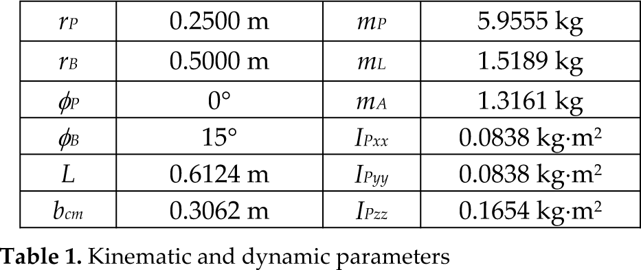
The robot is working up-side-down (Figure 6). The kinematic and dynamic parameters are shown in Table 1.

Figure 6.

Schematic representation of the manipulator and the workpiece

Table 1.

Kinematic and dynamic parameters

r_P	0.2500 m	m_P	5.9555 kg
r_B	0.5000 m	m_L	1.5189 kg
φ_P	0°	m_A	1.3161 kg
φ_B	15°	I_Pxx	0.0838 kg·m²
L	0.6124 m	I_Pyy	0.0838 kg·m²
b_cm	0.3062 m	I_Pzz	0.1654 kg·m²

The coordinates of the workpiece (position and orientation) are codified by real values through the vector $^{B} x_{W |_{B | E}} = {[\begin{matrix} x_{W} & y_{W} & z_{W} & ψ_{W} & θ_{W} & φ_{W} \end{matrix}]}^{T}$ . The solutions are randomly initialized in the workspace of the robot. The algorithm has a tournament-2 selection to determine the parents of the offspring [25]. After selection, the simulated binary crossover and mutation operators with p_c = 0.6 and p_m = 0.05 probabilities, respectively, are called [26].

In order to draw several different good solutions in one GA run, a ε strategy is used. The final solutions have all the same fitness value, but the values of the parameters are different from each other. At the end of each cycle, it is used a $ε - (λ + μ)$ strategy to select the solutions which survive for the next iteration. This means that the best solutions among parents and offspring are chosen. At this stage, the space is divided in hyper-planes separated by the distance ε and all solutions that fall into two consecutive hyper-planes are considered having the same preference, even if their fitness values are different. Two consecutive hyper-planes define a rank. In order to sort the solutions in a rank, the maximum selection is used. The ε value is initialized with 20 and is decreased during the evolution, until it reaches the value 0.003. The ε is decreased by 90% every time the best 200 solutions belong to the first rank and the value has not changed during the last 100 generations. The solutions are classified by the fitness function given by equation (34), in case the solution is admissible, otherwise the value 1×10²⁰ is assigned.

The algorithm draws a set of solutions that converge to a line with good diversity, corresponding to the location of the workpiece $^{B} x_{W |_{B | E}} = {[\begin{matrix} 0 & 0 & z_{W} & 0 & 0 & 0 \end{matrix}]}^{T}$ m. In fact, if there are no restrictions on the displacement of the actuators, any value is optimal for the z_W coordinate.

Figures 7 to 9 show the variation of P_act, along the trajectory, for the case where the workpiece is in its optimal location and z_W = 0.5 m.

Figure 7.

Variation of P_act as a function of x_P and y_P, for the optimal location of the workpiece

Figure 8.

Variation of P_act as a function of x_P and z_P, for the optimal location of the workpiece

Figure 9.

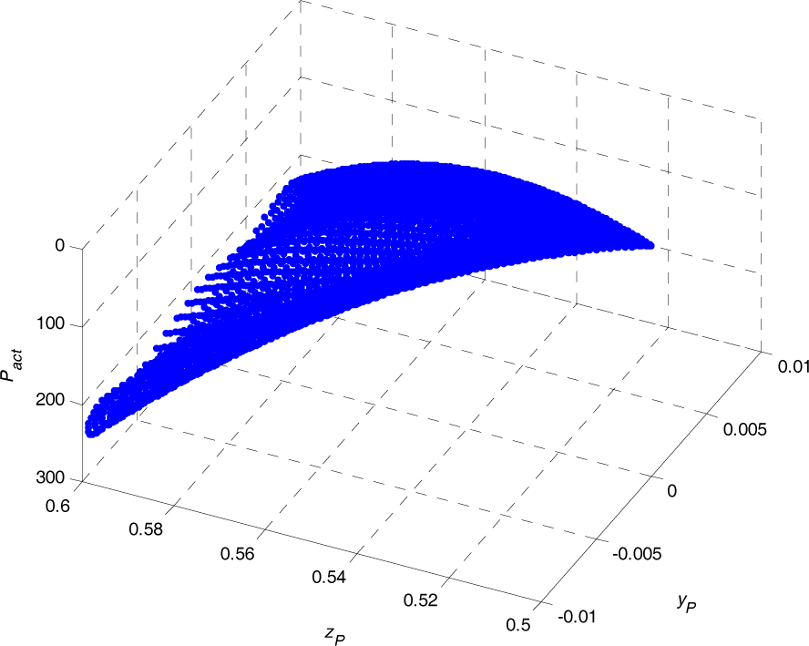
Variation of P_act as a function of y_P and z_P, for the optimal location of the workpiece

In Figures 10 to 12 we can see the variation of P_act, along the trajectory, for the case where the workpiece is away from its optimal location. It is clear that the required power in the actuators is higher than in the previous situation.

Figure 10.

Variation of P_act as a function of x_P and y_P, for the workpiece location [0.1 0.05 0.5 0 0 30°]^T

Figure 11.

Variation of P_act as a function of x_P and z_P, for the workpiece location [0.1 0.05 0.5 0 0 30°]^T

Figure 12.

Variation of P_act as a function of y_P and z_P, for the workpiece location [0.1 0.05 0.5 0 0 30°]^T

5.2. Multi-objective Optimization

Initially, GAs were designed to optimize single-objective problems. However, it was realized that, with some minor modifications, the algorithms could also solve problems involving, simultaneously, more than one objective [26]. To this end, GAs take advantage of their population to store a solution set representative of the non-dominated front. Thus, each population element is used to hold a non-dominated solution. Therefore, during the execution of the algorithm, the solutions are guided by the objective functions, using techniques that promote the dispersion of the solution [27] towards the non-dominated front. This kind of algorithms has been successfully used in many engineering problems, particularly in robotics [20, 28-29].

In this subsection, the mechanical power dissipated by the actuators, P_act, defined by equation (34), and the structural stiffness of the manipulator, given by equation (41), computed along the trajectory of the robot, are adopted as the optimization criteria. A multi-objective optimization algorithm, based on NSGAII [26], with maximin sorting scheme selection [30] is used. The crossover and mutation probabilities are p_c = 0.8 and p_m = 0.04, respectively. The search is carried out by a 100 elements population solution during 1000 generations.

Several independent optimizations were performed and the algorithm always converged to the same non-dominated front. Figure 13 illustrates one of the experiments, underlining one possible solution and the respective parameters. As can be seen, the two objectives are quarrelsome and several alternative solutions can be chosen as the desired workpiece position.

Figure 13.

Pareto front of optimal solutions

6. Conclusion

In a machining robotic cell, the best location for the workpiece to be machined depends on the task or, more precisely, on the trajectory and on the forces that the robot exerts on the workpiece. To find the best location, we formulate the problem as an optimization problem, and propose a GA to compute the optimal solution. Firstly we adopt a single objective function and then a multi-objective problem is considered. The described approach is absolutely generic and can be used with different optimization criteria and restrictions. This study didn't take into account the specific issues associated with the machining process, which determine the trajectory of the robot and the machining force. But the approach can be used for arbitrary trajectories and interaction forces.

References

Song

Chen

Y. H.

, “Feature-based robot machining for rapid prototyping,” Proceedings of the Institution of Mechanical Engineers, Part B: Journal of Engineering Manufacture, vol. 213, pp. 451–459, 1999.

Olabi

Béarée

Gibaru

Damak

, “Feedrate planning for machining with industrial six-axis robots,” Control Engineering Practice, vol. 18, pp. 471–82, 2010.

Abele

Weigold

Rothenbücher

, “Modeling and Identification of an Industrial Robot for Machining Applications,” Annals of the CIRP, vol. 56, pp. 387–390, 2007.

Huang

Lin

, “Rapid and flexible prototyping through a dual-robot workcell,” Robotics and Computer Integrated Manufacturing, vol. 19, pp. 263–272, 2003.

Brogardh

, “Robot Control Overview: An Industrial Perspective,” Modeling, Identification and Control, vol. 30, pp. 167–180, 2009.

Chen

Song

, “The development of a layer based machining system,” Computer-Aided Design, vol. 33, pp. 331–342, 2001.

Wall

Ulrich

Flowers

, “Evaluating prototyping technologies for product design,” Research Engineering Design, vol. 3, pp. 163–177, 1992.

Tangelder

Vergeest

, “Robust NC path generation for rapid shape prototyping,” Journal of Design and Manufacturing, vol. 4, pp. 281–292, 1994.

Kim

Park

Kim

, “Face sculpturing robot with recognition capability,” Computer-Aided Design, vol. 26, pp. 814–821, 1994.

10.

Guvenc

Srinivasan

, “An overview of robot-assisted die and mold polishing with emphasis on process modelling,” Journal of Manufacturing System, vol. 16, pp. 48–58, 1997.

11.

Milfelner

Kopac

Cus

Zuperl

, “Intelligent system for machining and optimization of 3D sculptured surfaces with ball-end milling,” Journal of Achievements in Materials and Manufacturing Engineering, vol. 14, 2006, pp. 171–177.

12.

Solvang

Refsahl

Sziebig

, “STEP-NC Based Industrial Robot CAM System,” In 9th International Symposium on Robot Control (SYROCO'09), Japan, 2009, pp. 361–366.

13.

Olsson

Haage

Kihlman

Johansson

Nilsson

Robertsson

Björkman

Isaksson

Ossbahr

Brogardh

, “Cost-efficient drilling using industrial robots with high-bandwidth force feedback,” Robotics and Computer-Integrated Manufacturing, vol. 26, 2010, pp. 24–38.

14.

Vosniakos

Matsas

, “Improving feasibility of robotic milling through robot Placement optimisation,” Robotics and Computer-Integrated Manufacturing, vol. 26, 2010, pp. 517–525.

15.

Mitsi

Bouzakis

K.D.

Sagris

Mansour

, “Determination of optimum robot base location considering discrete end-effector positions by means of hybrid genetic algorithm,” Robotics and Computer-integrated Manufacturing, vol. 24, 2008, pp. 50–59.

16.

Zaghbani

Lamraoui

Songmene

Thomas

El Badaoui

, “Robotic High Speed Machining of Aluminium Alloys,” Advanced Materials Research, vol. 188, 2011, pp. 584–589.

17.

Sugita

Nakano

Kato

Nakajima

Mitsuishi

, “Tool Path Generator for Bone Machining in Minimally Invasive Orthopaedic Surgery,” IEEE/ASME Transactions on Mechatronics, vol. 15, 2010, pp. 471–479.

18.

Barbosa

M. R.

Pires

E. J. Solteiro

Lopes

A. M.

, “Optimization of parallel manipulators using evolutionary algorithms,” In Soft Computing Models in Industrial and Environmental Applications, 5th International Workshop (SOCO 2010), Guimarñes, 2010, pp. 79–86.

19.

Rao

, “Dimensional synthesis of a spatial 3-RPS parallel manipulator for a prescribed range of motion of spherical joints,” Mechanism and Machine Theory, vol. 44, 2009, pp. 477–486.

20.

Chen

Pham

, “Trajectory planning in parallel kinematic manipulators using a constrained multi-objective evolutionary algorithm,” Nonlinear Dynamics, DOI 10.1007/s11071-011-0095-2.

21.

Chen

Liao

, “A hybrid strategy for time- and energy efficient trajectory planning for parallel platform manipulators,” Robotics and Computer-Integrated Manufacturing, vol. 27, 2011, pp. 72–81.

22.

Merlet

J-P

Gosselin

, “Nouvelle Architecture pour un Manipulateur Parallele a Six Degres de Liberte,” Mechanism and Machine Theory, vol 26, pp. 77–90, 1991.

23.

Lopes

A. M.

, “Dynamic modeling of a Stewart platform using the generalized momentum approach,” Communications in Nonlinear Science and Numerical Simulation, vol. 14, pp. 3389–3401, 2009.

24.

Holland

J. H.

Adaptation in Natural and Artificial Systems: An Introduction analysis with Applications to Biology, Control, and Artificial Intelligence. MIT Press, 1992.

25.

Michalewicz

Fogel

, How to solve it: Modern heuristics. New York: Springer-Verlag, 2000.

26.

Deb

, Multi-Objective Optimization Using Evolutionary Algorithms. Chichester: John Wiley & Sons, 2001.

27.

Laumanns

Thiele

Deb

Zitzler

, “Archiving with guaranteed convergence and diversity in multi-objective optimization,” In Proceedings of the Genetic and Evolutionary Computation Conference, pp. 439–447, 2002.

28.

Pires

E. J. Solteiro

de Moura Oliveira

P. B.

Machado

J. A. Tenreiro

, “Multi-Criteria Optimization Manipulator Trajectory Planning,” Robot Manipulators New Achievements, pp. 503–522, InTech, 2010.

29.

Ghanbari

Noorani

, “Optimal Trajectory Planning for Design of a Crawling Gait in a Robot Using Genetic Algorithm,” International Journal of Advanced Robotic Systems, vol. 8, pp. 29–36,2011.

30.

Pires

E. J. Solteiro

de Moura Oliveira

P. B.

Machado

J. A. Tenreiro

, “Multi objective MaxiMin Sorting Scheme,” Lecture Notes in Computer Science, vol. 3410/2005, pp. 165–175, 2005.

Optimization of the Workpiece Location in a Machining Robotic Cell

Abstract

Keywords

1. Introduction

2. Robot Kinematics

3. Robot Dynamics

3.1. Manipulator Kinetic Energy

3.1.1. Moving Platform Kinetic Energy

3.1.2. Actuators Kinetic Energy

3.1.3. Fixed-length Links Kinetic Energy

4. Objective Functions

5. Optimization

5.1. Single-objective Optimization

5.2. Multi-objective Optimization

6. Conclusion

References