
Abstract
This article presents an intelligent algorithm based on extreme learning machine and sequential mutation genetic algorithm to determine the inverse kinematics solutions of a robotic manipulator with six degrees of freedom. This algorithm is developed to minimize the computational time without compromising the accuracy of the end effector. In the proposed algorithm, the preliminary inverse kinematics solution is first computed by extreme learning machine and the solution is then optimized by an improved genetic algorithm based on sequential mutation. Extreme learning machine randomly initializes the weights of the input layer and biases of the hidden layer, which greatly improves the training speed. Unlike classical genetic algorithms, sequential mutation genetic algorithm changes the order of the genetic codes from high to low, which reduces the randomness of mutation operation and improves the local search capability. Consequently, the convergence speed at the end of evolution is improved. The performance of the extreme learning machine and sequential mutation genetic algorithm is also compared with that of a hybrid intelligent algorithm, and the results showed that there is significant reduction in the training time and computational time while the solution accuracy is retained. Based on the experimental results, the proposed extreme learning machine and sequential mutation genetic algorithm can greatly improve the time efficiency while ensuring high accuracy of the end effector.
Keywords
Introduction
The inverse kinematics of a robotic manipulator can be used to describe the mapping of the manipulator and end effector from the Cartesian space to joint space. It is crucial to obtain highly accurate inverse kinematics solutions in an efficient manner in the design, motion planning, and control of the manipulator.
1
–3
The main problem in determining the inverse kinematics solution of a robotic manipulator is to compute each joint angle
Determining the inverse kinematics solution of a robotic manipulator with a high degree of freedom (DOF) is a complex process. There are three types of methods typically used to determine the inverse kinematics solution of a robotic manipulator, namely, geometric, algebraic, and iterative algorithms. Each method has its own disadvantages. For example, algebraic methods cannot guarantee a closed-form solution. Geometric methods can be used to solve the inverse kinematics problem only when the first three joints of the manipulator have a closed-form solution. The convergence speed of iterative algorithms is dependent on the initial position of the robotic manipulator. In addition, due to the complex geometry of the structure, most methods are unable to determine the inverse kinematics solution of the robotic manipulator in a fast, efficient manner. Hence, much effort has been made by researchers to develop intelligent algorithms in order to compute the inverse kinematics solutions of robotic manipulators. Among these intelligent algorithms, artificial neural networks (ANNs) and genetic algorithms (GAs) have gained much attention from researchers in order to solve inverse kinematics problems of robotic manipulators.
Recently, many researchers proposed neural network-based inverse kinematics solutions of robotic manipulators. 4 –6 It has been proven theoretically that neural networks with three or more layers can fit any nonlinear system and this forms the basis that ANNs can be used to solve the inverse kinematics problems of robotic manipulators. Tejomurtula and Kak 7 presented a structured ANN to solve the inverse kinematics problem of a robotic manipulator, which prevents the shortcomings of the backpropagation algorithm in terms of the training time and computational accuracy. Karlik and Aydin 8 used six independent ANNs with two hidden layers to compute the inverse kinematics solution of a 6-DOF manipulator. Kalra et al. 9 proposed a new evolutionary approach to solve the multimodal inverse kinematics. This algorithm realizes high real-time and robust control of the inverse kinematics of the robotic manipulator. Bingul et al. 10 proposed an inverse kinematics algorithm based on backpropagation ANN. This method is disadvantageous because of the large joint angle errors and moreover, the method is incapable of handling multiple solutions. Rasit Köker and Tarık Cakar 11 –15 proposed a variety of hybrid intelligent algorithms based on ANN, GA, and simulated annealing (SA). In their studies, ANN was used to compute a preliminary solution and the fractional part of the inverse kinematics solution was optimized by GA or SA. However, the algorithms are still lacking in terms of the time efficiency because the training process of the ANN is rather slow while the optimization process based on the improved GA and SA requires a significant number of iterations to obtain a converged solution with high accuracy. A number of researchers have also proposed inverse kinematics solutions based on genetic GAs 9,16 and artificial bee colony algorithms. 17 These optimization algorithms search in the solution space subject to certain rules and the convergence speed is unsatisfactory in most situations. All of the aforementioned algorithms suffer from the same fundamental problem: the iteration process is time-consuming.
In this article, an intelligent algorithm is proposed based on extreme learning machine (ELM) and sequential mutation genetic algorithm (SGA) to determine the inverse kinematics solution of a 6-DOF robotic manipulator. The main focus of this novel approach is to improve the time efficiency of the algorithm while ensuring high precision of the end effector inverse kinematics. In this algorithm, forward kinematics is used to compute a training set from the joint space
The remainder of this article is organized as follows. The 6-DOF MT-ARM robotic manipulator used in the experiments and the fundamental theories pertaining to the forward kinematics of the robotic manipulator, ELM, and GA are presented in the “Preliminaries” section. In the “Proposed algorithm” section, we will describe in detail the proposed inverse kinematics solution of the robotic manipulator by integrating ELM with SGA, named the ELM-SGA algorithm. In the “Results and discussion” section, we present and compare the simulation and experimental results obtained using the proposed algorithm (ELM-SGA) and mainstream algorithm (Hybrid). Finally, the conclusions drawn based on the findings of the ELM-SGA algorithm are presented in the “Conclusions” section.
Preliminaries
Structure and Denavit–Hartenberg parameters of the 6-DOF Stanford MT-ARM robotic manipulator
The simulations and experiments are designed based on the 6-DOF Stanford MT-ARM robotic manipulator shown in Figure 1. The Denavit–Hartenberg method is used to analyze the kinematics of the manipulator. The basic strategy involves establishing the space coordinate system for each joint and then compute the conversion matrix between the adjacent joint coordinates. The final transformation matrix from the joint space of the manipulator to the Cartesian space of the end effector was calculated by the matrix transfer between each adjacent joint.
18
The four Denavit–Hartenberg parameters

Six-DOF Stanford MT-ARM robotic manipulator. DOF: degree of freedom.
Denavit–Hartenberg parameters of the 6-DOF Stanford MT-ARM robotic manipulator.

DOF: degree of freedom.
Forward kinematics of the 6-DOF Stanford MT-ARM robotic manipulator
The forward kinematics of a robotic manipulator can be described by the mapping from the joint space to the Cartesian space. 19 The forward kinematics of a robotic manipulator is usually analyzed by the Denavit–Hartenberg method, which establishes the coordinates for each joint and then calculates the position matrix by transformation between each adjacent joint coordinate. 20 The key aspect of the robotic manipulator forward kinematics is the matrix transformation between the adjacent joint coordinates. This is the well-known Denavit–Hartenberg transformation notation, which is given by
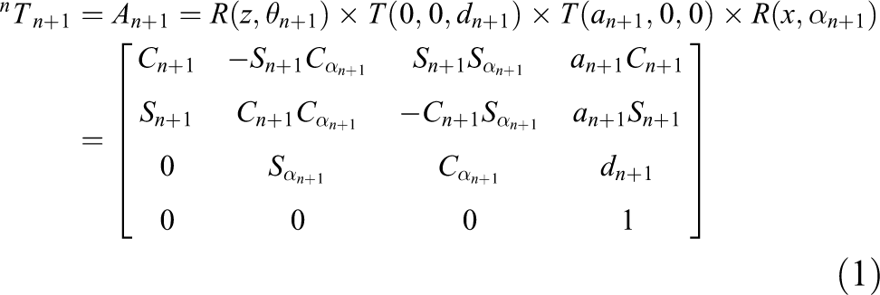
where

where


Extreme learning machine
ELM 21 –23 is the learning algorithm for single hidden layer neural networks proposed by Huang et al. 21 in 2006. As a single hidden layer feedforward neural network (SLFN), the training phase of the ELM consists of two stages: (1) random feature mapping and (2) solution of the linear parameters. In the first stage, ELM randomly initializes the hidden layer to map the input data into a feature space using nonlinear mapping functions, which can be any nonlinear piecewise continuous functions. 24,25 In ELM, the weights of the input layer and biases of the hidden layer are randomly initialized and they are not adjusted during the training process. In order to achieve better results, the weights of the input layer and biases of the hidden layer are set within a range of [−1, 1] and [−1, 1], respectively, during random initialization. Hence, ELM can greatly improve the training speed compared with conventional neural networks. The fundamental theory of ELM is briefly described as follows.
For N arbitrary distinct samples (Xi
, Ti
), where

where

This equation can be expressed in matrix form as follows

where


where H is the output matrix of the hidden layer, β is the output weight matrix, and T is the target matrix. It shall be noted that Wi and bi are randomly initialized. Thus, the sole target of the training process is to compute the output weight matrix β, which can be easily determined using the least squares method. The formula is expressed as

where
Steps involved in the ELM algorithm.

Genetic algorithm
GA is a stochastic search optimization algorithm derived from the survival rules in the biological evolution theory. GA was first proposed by Holland 26 in 1975. The basic idea of GA is to optimize the object by genetic operations, crossover, and mutation, and then select the optimal genetic solutions according to the fitness function. 27 GA has been used extensively in optimization problems. However, conventional GA is usually less efficient than other optimization methods. To improve its computational efficiency, GA is integrated with other evolutionary algorithms. Köker and Cakar 11 used SA as an operator in GA to optimize the inverse kinematics solution of a robotic manipulator. Garg 28 developed a hybrid technique by integrating GA with particle swarm optimization to solve the constrained optimization problems. In this work, a sequential mutation operation is proposed to improve local search ability of GA in order to optimize the inverse kinematics solution of the 6-DOF Stanford MT-ARM robotic manipulator. The adaptive crossover rate and mutation rate are selected for the GA. First, numbers within a range of [0, 1] are randomly generated and then compared with the crossover rate and mutation rate. When the crossover rate and mutation rate are smaller than the randomly generated number, the number will cross and vary.
Proposed algorithm
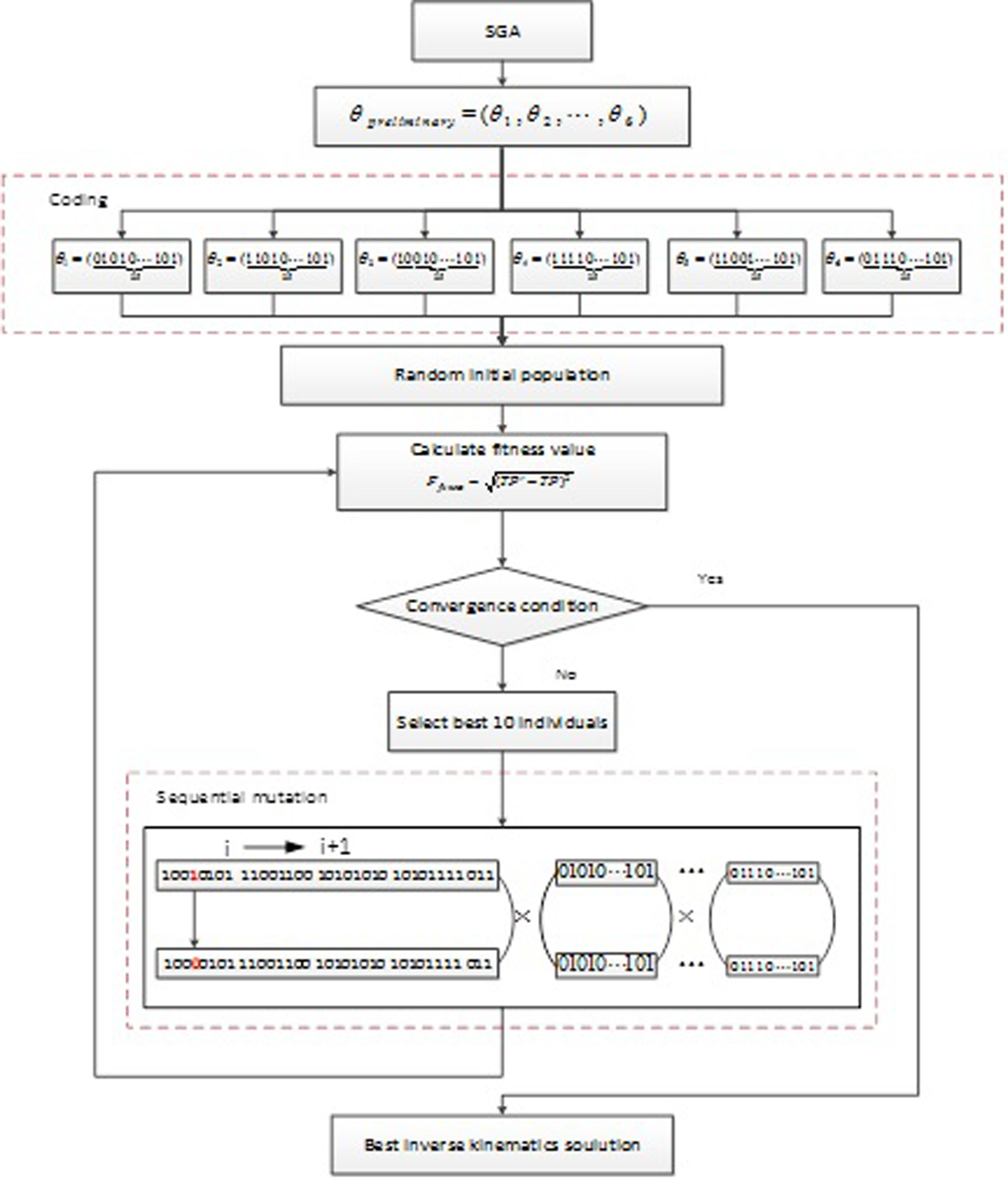
The proposed ELM-SGA algorithm used to determine inverse kinematics solution of the 6-DOF Stanford MT-ARM robotic manipulator is presented in this section. The main problem in inverse kinematics of robotic manipulators is to determine the joint angle

Flowchart of the proposed ELM-SGA algorithm used to compute and optimize the inverse kinematics solution of the robotic manipulator. ELM: extreme learning machine; SGA: sequential mutation genetic algorithm.
Computation of the preliminary inverse kinematics solution for 6-DOF Stanford MT-ARM robotic manipulator using ELM
As a single hidden layer neural network, ELM is designed to boost training speed. Unlike conventional neural networks, ELM randomly initializes the weights of input layer and biases of hidden layer only during the training process. This in turn reduces the training process. It is deemed reasonable that ELM sacrifices the accuracy of the preliminary inverse kinematics solution to a small extent in order to improve time efficiency. Solving the inverse kinematics problem using ELM consists of two stages: (1) training and (2) prediction. The training process is more crucial compared with the prediction process because it determines the success or failure of the prediction model. There are two issues that need to be considered during the training process. The first issue is to generate a suitable training data set, whereas the second issue is to select the appropriate number of hidden layers for the ELM model. Once the kinematic parameters of the robotic manipulator are known, a forward kinematics model can be formulated using equations (1)
to (14). To ensure rationality of the training set, the joint angles

Details of the training and prediction processes in the ELM algorithm. ELM: extreme learning machine.
Steps involved in the ELM algorithm to compute the preliminary inverse kinematics solution of the robotic manipulator.

Optimization of the inverse kinematics solution using SGA
The second stage of the proposed ELM-SGA algorithm involves optimizing the preliminary inverse kinematics solution. Even though GA is widely used for optimization problems, the crossover and mutation operations of GA process randomly, resulting in poor local search capability. Thus, conventional GA is not suitable to optimize highly precise preliminary inverse kinematics solutions, which only require micro adjustments during the optimization process. Hence, in this work, SGA is used to enhance the local search capability of GA, especially at the end of the evolution. In the SGA algorithm, the mutation operation is performed bit by bit from high to low. In each generation, the value of a specific bit is mutated and determined by the fitness function. The weight of the high bit is larger than that of the low bit and therefore, it has a greater contribution to the final solution. Thus, the local search capability of GA can be enhanced significantly with the SGA algorithm.
The details of the optimization process using SGA are as follows. First, the preliminary inverse kinematics solution


where
The artificial potential field method is chosen as the obstacle avoidance method. The environment in which the robot is located is defined by the potential field. The position information is used to control the robot arm in order to avoid obstacles. If the computed results indicate the possibility of collisions, the experimental results will be discarded. The computed results are retained if there are no collisions.
Next, the convergence criteria are set, which serve as the basis for termination of the SGA algorithm. In this work, the convergence criteria are determined by the maximum number of generations and a predefined tolerance value. When the maximum number of generations or the predefined convergence error is reached, the algorithm terminates the iterative loop. Fourth, in order to ensure the diversity of the population, the best 10 individuals are selected as the candidates. These individuals are then mutated in the order from high to low. For six joints and two mutation results (0 and 1), there are 2 6 different candidate individuals. In each generation, the SGA determines the value of the corresponding bit. The SGA then iterates from step 4 to 3 until the solution converges. Algorithm 3 shows the steps involved in the SGA algorithm used to optimize the inverse kinematics solution of the robotic manipulator. Figure 4 shows the flowchart of the SGA algorithm. Figure 5 shows the details of the mutation between the ith and (i + 1)th generations for one individual.
Steps involved in the SGA algorithm used to optimize the inverse kinematics solution of the robotic manipulator.

Flowchart of the SGA algorithm. SGA: sequential mutation genetic algorithm.

Details of the mutation between the ith and (i + 1)th generations.
Results and discussion
The performance of the proposed ELM-SGA algorithm in solving the inverse kinematics problem of the robotic manipulator is validated by performing simulations and experiments, which will be described in this section. The simulations are divided into three parts in order to determine the time efficiency during the training process, optimization process, and computational process. In part 1, the ELM and ANN models with different hidden layer nodes are compared in order to determine the performance of these models in computing the preliminary inverse kinematics solution of the robotic manipulator. The performance of the ELM and ANN models are assessed in terms of the training time and output MSE. In part 2, the proposed SGA and Hybrid 11 algorithms are compared in order to determine the performance of these algorithms in optimizing the preliminary inverse kinematics solution determined using the ELM and ANN models, respectively. The convergence process is assessed based on the end effector error. In part 3, the performance of the ELM, Hybrid, dual redundant camera robot based on genetic algorithm (DRCRB-GA), 12 and proposed ELM-SGA algorithms will be compared in detail. The ELM-SGA algorithm is then applied to the 6-DOF Stanford MT-ARM robotic manipulator in order to validate the performance of the algorithm. The final experiments consist of six experiments to validate the accuracy of different end effector poses as well as a fixed-point grasping experiment. The algorithms are coded using Visual Studio C++.NET 2003 on a personal computer installed with an Intel Core i7-4720HQ @2.60 GHz processor and the application framework uses the Microsoft Basic Class Library version 7.0 (i.e. the MFC library). The time points are set before and after the inverse kinematics solution is computed and the time difference between the two time points is used as an index to evaluate the time efficiency of the algorithms. Experiments are then performed on the 6-DOF Stanford MT-ARM modular robotic manipulator.
Comparison between ELM and ANN in computing the preliminary inverse kinematics solution of robotic manipulator
The performance between the ELM and ANN models in computing the preliminary inverse kinematics solution of a 6-DOF Stanford MT-ARM robotic manipulator is presented in this section. Figure 3 shows the processes involved in solving the inverse kinematics problem using the ELM model. In order to obtain the training set, the joint vector
To compare the performance of the ELM and conventional ANN models, seven data sets are recorded, including the training time and MSE. The initial number of nodes is 25 and the number of nodes is increased in steps of 50, as shown in Table 2. When the ELM model is used to compute the inverse kinematics solution of the MT-ARM robotic manipulator, it is found that the MSE of the output joint angle decreases with an increase in the number of hidden layer nodes. The MSE is 1.98028593 when the number of hidden layer nodes is 275. The corresponding training time is 0.3814 s. The simulations are repeated using the ANN model. Likewise, the MSE of the output joint angle decreases with an increase in the number of hidden layer nodes. The lowest MSE (1.65137561) is attained when the number of hidden layer nodes is 175, while the corresponding training time is 13.9127 s. Comparing the results obtained for the ELM model (275 hidden layer nodes) and ANN model (175 hidden layer nodes), it can be seen that the ANN model has a slightly higher precision than the ELM model. However, the training time for the ANN model is 4.36 times the training time for the ELM model. Figure 6(a) and (b) shows the variations of the MSE and training time for the ELM and ANN models. It is evident that the ANN model has a slightly higher accuracy than the ELM model. However, this is negated by the fact that the ANN model is more time-consuming compared with the ELM model, as indicated by the increasing trend in the training time (Figure 6(b)). The simulation results indicate that ELM model can significantly reduce the training time without compromising the accuracy of the solution since the precision of the output is comparable to that for the ANN model.
Comparison of the MSE and training time between the ANN and ELM models with different number of hidden layer nodes.

MSE: mean square error; ELM: extreme learning machine; ANN: artificial neural network.
Note: The bold values represent the minimum mean square error and the minimum training time in different algorithms.

Variations of the (a) MSE and (b) training time of the ANN and ELM models with different number of hidden layer nodes. MSE: mean square error; ANN: artificial neural network; ELM: extreme learning machine.
Optimization of inverse kinematics solution of the robotic manipulator using SGA
As described in the previous section, ELM is used to compute the preliminary inverse kinematics solution of the robotic manipulator. The main purpose of the ELM model is to reduce the training time. However, the end effector error obtained from the ELM model is on the order of a few centimeters, which is undesirable. Hence, SGA is used to optimize the preliminary inverse kinematics solution and the results will be presented and discussed in this section. Even though GA has been used extensively to solve optimization problems, the poor local search capability of GA reduces its convergence speed, especially at the end of the evolution. Hence, the SGA algorithm is used in this work to compensate the disadvantages of classic GA and promote its convergence speed. The SGA algorithm is used to optimize the preliminary inverse kinematics solution obtained from the ELM model. The coding, details of the sequential mutation, and end effector errors are recorded for each generation. The performance of the ELM-SGA and Hybrid 11 algorithms are compared in order to determine their convergence capability.
Table 3 shows the preliminary inverse kinematics solutions obtained by the ELM model and their corresponding binary formats based on the rules described in the “Optimization of inverse kinematics solution of the robotic manipulator using SGA” section. The binary format of each joint angle consists of a sign bit and 34 binary bits converted from the floating parts of each joint angle. After coding, the population is initialized, the fitness value is computed, the convergence criteria are evaluated, and the selection operations are run. The principle of SGA is the same as classic GA and therefore, the procedure will not be elaborated in detail in this section. The inverse kinematics solutions presented in Table 3 are taken as the example in order to demonstrate the sequential mutation process of the SGA, as shown in Figure 7. The evolutions between the fourth and fifth generations are recorded. In the fourth generation, the fourth bit (highlighted in red) mutates and generates 26 new individuals. The fitness value is then computed in order to identify which individuals are inherent to the next generation. To ensure diversity of the population, the algorithm does not select the best mutated individual as its offspring for each individual, rather the algorithm chooses a certain number of best fit individuals as the offspring.
Binary formats of the preliminary inverse kinematics solutions obtained from the ELM model.

ELM: extreme learning machine.
Note: The bold values indicate positive and negative signs, 0 for positive and 1 for negative.

Sequential mutation from the ith generation to (i + 1)th generation. MSE: mean square error; ANN: artificial neural network; ELM: extreme learning machine.
A hybrid intelligent algorithm based on ANN, GA, and SA is used to compare with the convergence ability of the ELM-SGA algorithm developed in this work during the optimization process. Köker and Cakar 11 proposed this hybrid intelligent algorithm to solve the inverse kinematics problem of a robotic manipulator in 2016. In the hybrid intelligent algorithm, ANN is used to compute the preliminary inverse kinematics solution. Following this, an improved GA with SA is used to optimize the inverse kinematics solution. In one study, 12 the DRCRB-GA algorithm is proposed by setting two variable parameters, which constrains two redundant DOFs. The structure of the optimized objective function is more flexible than the basic GA and the algorithm is shown to be more efficient. The ELM-SGA, DRCRB-GA, and Hybrid algorithms are used to compute the inverse kinematics solution for the same pose. The end effector errors are recorded for each of these algorithms in each generation.
Figure 8 shows the comparison of the convergence process between the SGA and Hybrid algorithms. The abscissa represents the algebra of Gas, whereas the ordinate represents the end effector error. The blue data markers represent the results of the Hybrid algorithm proposed by Köker and Cakar, 11 whereas the red data markers represent the SGA algorithm proposed in this study. Since the SGA uses the preliminary inverse kinematics solution determined by the ELM model, the accuracy of the solution is slightly lower compared with that for the ANN model. Therefore, the end effector error is larger for the SGA algorithm compared with that for the Hybrid algorithm at the beginning of the optimization process. However, the SGA algorithm has faster convergence speed than the Hybrid algorithm and the end effector error of the SGA algorithm begins to approach zero in the 29th generation. In contrast, the Hybrid algorithm achieves convergence in the 36th generation. This indicates that the proposed ELM-SGA algorithm improves the optimization of the inverse kinematics solution of a robotic manipulator.

Comparison of the convergence process between the SGA and Hybrid algorithms. SGA: sequential mutation genetic algorithm.
Comparison of the inverse kinematics solutions between the ELM, Hybrid, DRCRB-GA, and ELM-SGA algorithms for 10 different random poses
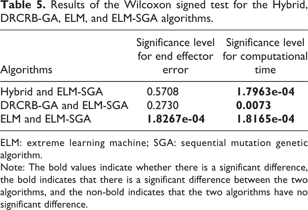
In order to prevent randomness of a single simulation, the ELM, Hybrid, DRCRB-GA, and proposed ELM-SGA algorithms are used to compute the inverse kinematics solutions for 10 random poses. The simulation results are presented in Table 4, including the average end effector error, standard deviation of the end effector error, average computational time, and standard deviation of the computational time. It can be seen from Table 4 that the accuracy of the inverse kinematics solution is significantly higher for the ELM-SGA algorithm compared with other algorithms, while the computational time is less than that those for the Hybrid and DRCRB-GA algorithms. Table 5 shows the results of the Wilcoxon signed test for the Hybrid, DRCRB-GA, ELM, and ELM-SGA algorithms. The significance level is 0.05. If the calculated significance level is less than 0.05, this indicates that the difference in the result between two algorithms is significant. In contrast, if the calculated significance level is greater than 0.05, this indicates that there is no significant difference in the result between two algorithms. Indeed, there is a significant difference in the time efficiency between the proposed ELM-SGA algorithm and other algorithms. In addition, there is a significant difference in error between the ELM-SGA and ELM algorithms. Based on the results, it can be deduced that the ELM-SGA algorithm can achieve the same accuracy as the Hybrid and DRCRB-GA algorithms, but with higher time efficiency compared with other algorithms.
Average end effector error and average computational time for the Hybrid, DRCRB-GA, ELM, and ELM-SGA algorithms.

ELM: extreme learning machine; SGA: sequential mutation genetic algorithm.
Results of the Wilcoxon signed test for the Hybrid, DRCRB-GA, ELM, and ELM-SGA algorithms.
ELM: extreme learning machine; SGA: sequential mutation genetic algorithm.
Note: The bold values indicate whether there is a significant difference, the bold indicates that there is a significant difference between the two algorithms, and the non-bold indicates that the two algorithms have no significant difference.
In order to compare the capability of the algorithms in computing the inverse kinematics solution, the end effector errors and computational time are plotted for the Hybrid, DRCRB-GA, and ELM-SGA algorithms, as shown in Figure 9. The red, blue, and green polylines in Figure 9(a) indicate the end effector errors for the ELM-SGA, Hybrid, and DRCRB-GA algorithms, respectively. The errors of the three algorithms fall within a range of 0.005–0.045 mm. The trajectory of the three polylines is very close and therefore, it can be deduced that the algorithms achieve the same accuracy. Even though the ELM-SGA algorithm can obtain a more precise inverse kinematics solution, the main concern here is the convergence speed of the algorithm. Thus, the convergence criterion is set such that the end effector error is less than 0.05 mm. The red, blue, and green polylines in Figure 9(b) indicate the computational time of the ELM-SGA, Hybrid, and DRCRB-GA algorithms, respectively. It can be seen that the ELM-SGA algorithm is less time-consuming compared with the Hybrid and DRCRB-GA algorithms, indicating that the proposed algorithm achieves faster convergence than other algorithms while attaining the same precision. Based on Table 4, the average computational time of the ELM-SGA algorithm is lower than those for the Hybrid and DRCRB-GA algorithms by 5.5% and 3.7%, respectively.
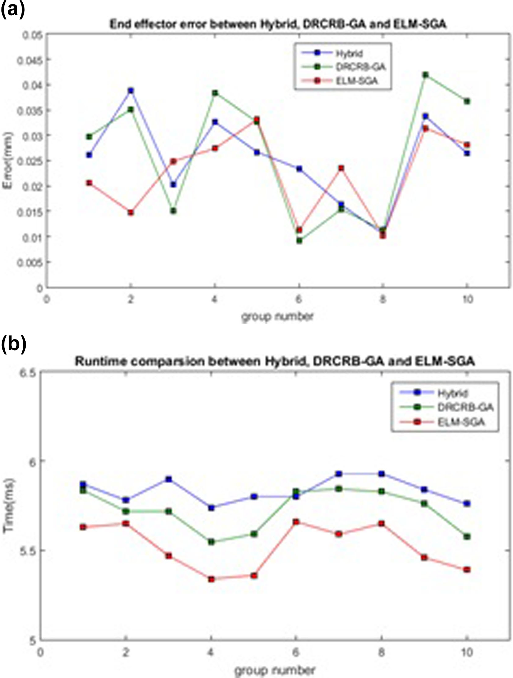
Comparison of the end effector errors and computational time between the Hybrid, DRCRB-GA, and ELM-SGA algorithms. ELM: extreme learning machine; SGA: sequential mutation genetic algorithm.
Experiments using the 6-DOF Stanford MT-ARM robotic manipulator
Two groups of validation experiments are conducted and the proposed ELM-SGA algorithm is used to determine the inverse kinematics solution of the Stanford MT-ARM robotic manipulator, which will be presented in this section. The robotic manipulator has been described in detail in the “Structure and Denavit–Hartenberg parameters of the 6-DOF Stanford MT-ARM robotic manipulator” section. In the first group of experiments, the forward kinematics of the robotic manipulator is used to verify the accuracy of the ELM-SGA algorithm in computing the inverse kinematics solution. In the second group of experiments, the ELM-SGA algorithm is used to compute the inverse kinematics solution in order to realize fixed-point grasping of the robotic manipulator.
End effector errors for six poses of the robotic manipulator obtained from ELM-SGA algorithm
In this section, the proposed ELM-SGA algorithm is applied to the 6-DOF Stanford MT-ARM robotic manipulator to verify the accuracy of the inverse kinematics solution. Each joint angle of the robotic manipulator is set equidistantly from 15° to 90° with a pitch of 15° and the pose data T returned by the robotic manipulator is recorded. The ELM-SGA algorithm is then used to compute the inverse kinematics solution θ for each pose T. The inverse kinematics solutions obtained are set as the joint parameters of the robotic manipulator. The error between the observed pose T ′ and expected pose T of the end effector (i.e. end effector error) is calculated using equation (22) in order to verify the accuracy of the ELM-SGA algorithm.
The results shown in Table 6 indicate that the ELM-SGA algorithm yields highly precise inverse kinematics solutions for the 6-DOF Stanford MT-ARM robotic manipulator. Figure 10 shows the six poses of the robotic manipulator corresponding to the inverse kinematics solutions tabulated in Table 6. In general, all of the end effector errors are less than 5 mm. The end effector errors are contributed by the following factors: (1) error between the inverse kinematics solution obtained by the ELM-SGA algorithm and ideal inverse kinematics solution whose end effector error relative to the target position equals zero and (2) accuracy of the arm-drive motor as well as drawbacks of the software control system. The input parameters of the MT-ARM robotic manipulator must be rounded to the nearest integer, which is the major contributor of the errors listed in Table 6. In summary, the error contributed by the ELM-SGA algorithm is less than 5 mm and therefore, it can be deduced that the proposed algorithm is capable of giving highly precise inverse kinematics solutions.
Validation of the inverse kinematics solutions obtained from the ELM-SGA algorithm for six poses.

ELM: extreme learning machine; SGA: sequential mutation genetic algorithm

Validation of the inverse kinematics solutions obtained from the ELM-SGA algorithm for six poses using the 6-DOF Stanford MT-ARM robotic manipulator. DOF: degree of freedom; ELM: extreme learning machine; SGA: sequential mutation genetic algorithm.
Fixed-point grasping experiments based on the ELM-SGA algorithm
Fixed-point grasping experiments are conducted to verify the accuracy of the inverse kinematics solutions obtained from the ELM-SGA algorithm. The experimental procedure is described as follows. First, a set of joint angles

Fixed-point grasping experiments using the 6-DOF Stanford MT-ARM robotic manipulator. DOF: Degree of freedom.
Parameters of the fixed-point grasping experiments.

Conclusions
An intelligent ELM-SGA algorithm has been proposed in this article in order to obtain the inverse kinematics solutions of a 6-DOF robotic manipulator. This is the first time ELM is used to compute the inverse kinematics solution of a 6-DOF robotic manipulator. The proposed ELM-SGA algorithm computes the inverse kinematics solution of the robotic manipulator in two stages. In the first stage, ELM is used to compute the preliminary inverse kinematics solution. In the second stage, SGA is used to optimize the preliminary inverse kinematics solution obtained from the ELM model. ELM randomly initializes the weights of the input layer and biases of the hidden layer, which greatly improves the training speed. Sequential mutation significantly improves the local searching capability of the GA. The ELM-SGA algorithm sacrifices the accuracy of preliminary inverse kinematics solution to a small extent, which significantly reduces the training time. The simulation and experimental results indicate that the ELM-SGA algorithm significantly improves the computational time without compromising the accuracy of the inverse kinematics solution of the robotic manipulator.
Footnotes
Declaration of conflicting interests
The author(s) declared no potential conflicts of interest with respect to the research, authorship, and/or publication of this article.
Funding
The author(s) disclosed receipt of the following financial support for the research, authorship, and/or publication of this article: This work is supported by Zhejiang Provincial Natural Science Foundation of China (no. LY18F030018, LZ15F020004), Natural Science Foundation of China (no. 51376055, 61272311), 521 Plan of Zhejiang Sci-Tech University, and Science and Technology Plan of Zhejiang Province (no. 2017C31017).