Sage Journals: Discover world-class research

Abstract

To make robots coexist and share the environments with humans, robots should understand the behaviors or the intentions of humans and further predict their motions. In this paper, an A^*-based predictive motion planner is represented for navigation tasks. A generalized pedestrian motion model is proposed and trained by the statistical learning method. To deal with the uncertainty, a localization, tracking and prediction framework is also introduced. The corresponding recursive Bayesian formula represented as DBNs (Dynamic Bayesian Networks) is derived for real time operation. Finally, the simulations and experiments are shown to validate the idea of this paper.

Keywords

Navigation Behavior Learning Behavior Understanding Mobile Robots Anytime Planning

1. Introduction

By the efforts of robotic researchers, there has been a great progress in robotic techniques. Robots no longer only work in laboratories or factories. Lots of novel robots were designed and developed to work in the populated or outdoor environments [1, 30, 37] in the last two decades. Different kinds of service robots provided assistance to people in hospitals [5], home environments [13, 24], shopping malls [17], building cleaning [36], and museums [4, 27, 32].

Navigation is one of the most important fundamental techniques for mobile robots. Service robots usually work in the crowded and highly dynamic environments, as shown in Figure 1. Time for deliberation is limited and planning is required to be fast and efficient. Moreover, in human society, the service robots should not only consider the obstacle avoidance but also understand the social effects of pedestrians [10, 20–21, 25, 28, 33].

Figure 1.

Service robots usually work in the crowded environments

Since the actions of pedestrians are usually uncertain, configuration space will be highly transitory. Traditional motion planning which queries a complete path from current position to the goal often takes too much time to satisfy the real time requirement. Thus, lots of researchers developed efficient replanning algorithms to cope with the real time challenge [9, 18, 29, 38]. By feeding the updated information, the original path is modified as a more appropriated one. However, when the planning problem is complex, a complete and optimal path may not be easily found within the limited deliberation time. Anytime algorithms are useful and have been shown the excellent results in this situation [14, 19]. It generates a suboptimal path quickly in the beginning and further improves the path until the deliberation time has run out.

Moreover, planning horizon also influences the navigation performance. Although the reactive motion planning [15–16, 23, 35] was able to rapidly query the next appropriate action, it still easily got blocked in complex cases because of its greedy property. In contrast, a look-ahead planner can efficiently decrease the probability of collision. By offering the ability of prediction, it is easier to avoid emergency events during the navigation period. Besides time limitation and planning horizon, uncertainty is another consideration for planning problem in real world. The control actions are usually non-deterministic. The sensor measurements are sometimes noisy and incomplete and cannot obtain the full states of the environment. In other words, the planner must cope with current uncertainty and even the uncertainty the robot may suffer in the future. POMDPs (Partially Observable Markov Decision Processes) is a general framework that addresses both the uncertainty in actions and perceptions. Unfortunately, the exact POMDPs solution is computationally involved and is hard to be implemented in real time. Although a lot of approximated methods were proposed, they were still mainly focused on the high level planning in small state space or simple environments [11, 22]. Thus, in this paper, the proposed planning algorithm is not addressed in the POMDPs framework. Instead, all the uncertainties are represented as costs in the configuration time space(C-T Space) and the trajectory is queried by the planner over this space.

Three main topics are discussed in this paper. The first part is focused on learning of the pedestrian motion model. A gird-based pedestrian motion model is utilized to predict the long term pedestrian motion. In the second part, a framework of Dynamic Bayesian Networks (DBNs) is derived for localization, tracking and prediction. Finally, a predictive motion planner is developed for dynamic environments. The sections in this paper also follow these three topics. In section 2, we introduce the structure and the learning methods of the pedestrian model. In section 3, a generalized probabilistic framework is derived for localization, tracking and prediction. In section 4, a predictive A^* planner is described. Simulations and experiments are given in section 5 to validate the proposed planner. Finally, conclusions are summarized in section 6.

2. Pedestrian Model Learning

To predict the actions of pedestrians, one of the best ways is to recognize the pedestrian motion model. In the short term prediction, we can easily utilize certain motion models, such as constant velocity model or constant acceleration model, to predict the next position of pedestrians. However, in the long term prediction, it is not obvious to define a motion pattern. Several previous researches had discussed and developed different methods for pedestrian model learning. Most of them emphasized the goal-directed concept to predict the pedestrian motion. By recognizing the potential goals that people might go forward, it is able to further predict their motions in the next few seconds. For example, Foka [12] predicted the human motion by manually defining the “hot points” where people may approach in daily life. Bennewitz [2] used expectation maximum(EM) to cluster the collected pedestrian trajectories and obtain the potential goals leading the movement of human in the environment. He further derived a Hidden Markov Model (HMM) to estimate the motion of people. Yen [34] extracted the potential goals of environment by clustering the trajectories with K-means. A navigation function (NF) is used to provide suggestions on pedestrian motion. The transition probabilities of gradient direction based on NF are available with statistically analyzing the frequency of certain directions led by NF. This method can efficiently model the pedestrian motions in the certain place after locating the potential goals.

However, the above methods are required either define potential goals manually or recollect the trajectories while environments are different. These processes are tedious and time-consuming. In general, the environment structures are similar in the same building. The size of doors and corridors are all similar. Our purpose is to learn a generalized pedestrian motion model. It allows the robot to work in different but similar places without recollecting new trajectories or re-training the motion model.

It needs to be emphasized that the interaction between the robot and pedestrians are not considered in our pedestrian model. Since our main purpose is navigation, the robot should minimize the robot-human hindrances and always avoid the potential collisions.

2.1 Potential Goal Extraction

Most potential goals are correlated to the environment structures. In this paper, the GVG (Generalized Voronoi Graph) [6] is used to automatically extract most potential goals. Potential goals that cannot be detected by environment structure are assigned manually. The environment map is divided into several submaps. Each submap has its exits which are regarded as the potential goals. The criteria of map division are based on the characteristics of geometry. For example, Figure 2(b) shows five submaps and extracted potential goals. The similar work was proposed by Thrun [31] which was focused on the topological map extraction. Moreover, after map division, the navigation function (NF) of every potential goal in submaps is calculated. Meanwhile, the distance map (DistMap), which represents the distance from a grid location to its closest obstacle, is also evaluated. Figure 2(c)(d) show the NF and DistMap of the blue submap.

Figure 2.

Map division. (a) environment map, (b) GVG structure and critical points, (c) NF of potential goal 2 in the blue submap, (d) distance map of the blue submap.

2.2 Generalized Pedestrian Motion Model

In fact, it is not easy to accurately predict the long term trajectory of the pedestrian. Instead of predicting an accurate trajectory, the proposed pedestrian model predicts the occupied probability of the specified area. Similar to Yen [34], we also utilize NF as the framework. NF can be regarded as a function of distance to the goal. An example for 8-neighbor NF is shown in Figure 3 (a) and the goal is marked as “G”. By transferring the map into grid space, the location of the pedestrian can be represented as one of the grids. Every grid state has 8 neighbors which are considered as the next potential directions. NF provides the suggestions and at least one optimal direction in each grid shown in Figure 3(b). From the relative angle to the optimal direction, several directional lots are grouped in each 45 degrees. For example, there are five lots in Figure 3(c).

Figure 3.

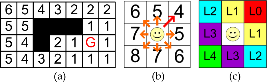
(a) navigation function. Black grids are occupied by obstacles, (b) NF model. The best direction denoted by the long red arrow, (c) NF-based pedestrian motion model. Five directional lots are grouped.

To illustrate the relationships among NF, DistMap and environments, 32 trajectories of pedestrians were collected and shown in Figure 4(a)-(b). Figure 4(c) denotes the histogram of lots with different distance to goals. It can be seen that pedestrians often follow the directions of lot0 and lot1 which are marked as blue lines and red lines. Only when the pedestrians approach the goal, the percentage of other directions will increase. The reason is that the goal is sometimes located in the corners or doorways, people usually “detour” the corners to prevent the potential collisions and violate the optimal directions suggested by NF. Besides, one might notice that only few paths are close to the wall. It is reasonable since people naturally tend to walk in a path that gives ample clearance from obstacles, rather than passing very close to them.

Figure 4.

(a) environment picture, (b) 32 trajectories collected by a laser range finder. lot0: blue line, lot1:red line, lot2:green dot, lot3: black dot, (c) statistical results of different lots.

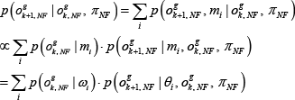
All the above evidence indicates that the use of two features, distance to goal and distance to obstacle, is able to construct a more generalized pedestrian model. Here, we draw the pedestrian motion model as p(o_k+1|o_k,G). o_k and o_k+1 indicate the states of the pedestrian in continuous space at time step k and k+1. G is the goal of the pedestrian. It covers the information for corresponding NF and DistMap. Since the pedestrian model is built on the grid space, the state of pedestrian is discretized and represented as ^{o
_k
^g} in this paper. Thus the pedestrian model in grid space can be rewritten as p(o^g_k+1 | o^g_k, G). We assume that the information can be factorized by NF and DistMap (denoted as π_NF and π_DistMap). The pedestrian model can be represented as Eq. (1)

\begin{array}{l} \begin{array}{l} p (O_{k + 1}^{g} | O_{k}^{g}, G) \\ = p (O_{k + 1, N F}^{g}, O_{k + 1, D i s t M a p}^{g} | O_{k, N F}^{g}, O_{k, D i s t M a p}^{g}, π_{N F}, π_{D i s t M a p}) \\ = p (O_{k + 1, D i s t M a p}^{g} | O_{k, D i s t M a p}^{g}, π_{D i s t M a p}) \cdot p (O_{k + 1, N F}^{g} | O_{k, N F}^{g}, π_{N F}) \end{array} \end{array}

(1)

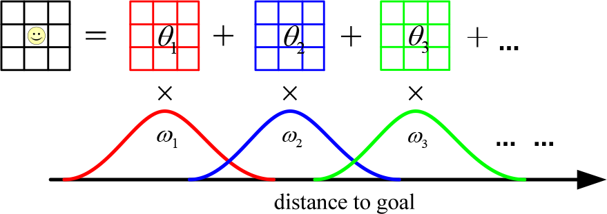
o^g_i,DistMap is the distance from o^g_i to the closest obstacles p(o^g_k+1,DistMap | o^g_{k, DistMap}, π_DistMap) and p(o^g_k+1,NF | o^g_k,NF, π_NF) are the motion models in DistMap and NF. In NF motion model, it further leads to a parameter m, called motion primitive. Each motion primitive m has its weighting factor i and transition probabilities of directional lots θ_i. According to total probability and Bayes rule, p(o^g_k+1,NF | o^g_k,NF, π_NF) can be further derived as

\begin{array}{l} p (o_{k + 1, N F}^{g} | o_{k, N F}^{g}, π_{N F}) = \sum_{i} p (o_{k + 1, N F}^{g}, m_{i} | o_{k, N F}^{g}, π_{N F}) \\ \propto \sum_{i} p (o_{k, N F}^{g} | m_{i}) \cdot p (o_{k + 1, N F}^{g} | m_{i}, o_{k, N F}^{g}, π_{N F}) \\ = \sum_{i} p (o_{k, N F}^{g} | ω_{i}) \cdot p (o_{k + 1, N F}^{g} | θ_{i}, o_{k, N F}^{g}, π_{N F}) \end{array}

(2)

Now p(o^g_k+1,NF | o^g_k,NF, π_NF) can be viewed as the linear combination with different motion primitives (Figure 6). The weighting factor i of each motion primitive is modeled as a Gaussian distribution. In other words, the motion model in NF can be viewed as a Gaussian Mixture Model.

2.3 Pedestrian Model Learning

According to Eq. (1), the pedestrian model is factorized into motion model in DistMap and NF. The learning methods will be discussed.

(a) Motion Model in DistMap

To estimate the parameters of the motion model in DistMap, the frequency of certain distance in DistMap is statistically analyzed. Here the probability from distance i to distance j is marked as p_ij and can be estimated by

p_{i j} = p (D_{j}^{​} | D_{​_{i}}^{​}, π_{D i s t M a p}) = \frac{t h e n u m b e r o f D_{i j}}{t h e n u m b e r o f D_{i}}

(3)

where D_i: distance i; D_ij: from distance i to distance j

(b) Motion Model in NF

We utilize EM (expectation-maximization) to estimate the parameters of the motion model in NF. The parameters include the probabilities of lots θ in each motion primitive and the corresponding weighting factor ω with a Gaussian distribution N(μ_i, ∑_i).

EM is an iteratively optimization algorithm which involves two steps, E-step and M-step. In E-step, the responsibilities γ_ni are evaluated by current parameters.

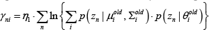
γ_{n i} = η_{1} \cdot \sum_{n} \ln {\sum_{i} p (z_{n} | μ_{i}^{o l d}, Σ_{i}^{o l d}) \cdot p (z_{n} | θ_{i}^{o l d})}

(4)

where η¹ is the normalized factor. γ_ni is the responsibility of data point z_n for motion primitive m_i. In M-step, the parameters are estimated with corresponding responsibilities γ_ni as

μ_{i}^{n e w} = η_{2} \sum_{n} γ_{n i} \cdot z_{n}

(5)

Σ_{i}^{n e w} = η_{2} \sum_{n} γ_{n i} \cdot (z_{n} - μ_{i}^{n e w}) \cdot (z_{n} - μ_{i}^{n e w})

(6)

θ_{i}^{n e w} (l o t_{j}) = η_{3} \cdot \sum_{n} p (z_{n} (l o t_{j}) | μ_{i}^{n e w}, Σ_{i}^{n e w})

(7)

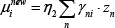
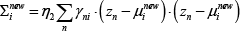
where η₂, η₃ are normalized factors. θ^new_i (lot_j) is the probability of lot_j in θ^new_i η x_n(lot_j) is the data point z_n with direction lot_j.

In order to learn the parameters of the pedestrian model, ninety nine trajectories are collected from three different but similar corridor environments, as shown in Figure 5 . 5103 data points are extracted from those trajectories. Now the motion model in NF can be viewed as the linear combination of motion primitives, as shown in Figure 6 . To choose the number of motion primitives K, the likelihoods of the pedestrian models with different K are compared and shown in Figure 7 . Cross validation is applied to prevent overfitting problem. Considering the compactness and modeling performance, K=5 is chosen in this paper. The estimated parameters are listed in Table 1.

Figure 5.

Ninety nine trajectories collected from different environments.

Figure 6.

the motion model in NF can be viewed as the linear combination of motion primitives.

Figure 7.

the fitness score with different number of motion primitives

Table 1.

Motion primitives. p(lot_i) indicates the probability of lot_i. Unit of μ: meter.

	μ	∑	p(lot0)	p(lot1)	p(lot2)	p(lot3)
m0	1.330	1.629	0.247	0.568	0.099	0.084
m1	2.871	2.078	0.276	0.532	0.139	0.051
m2	4.811	2.779	0.522	0.405	0.033	0.039
m3	6.926	6.486	0.414	0.565	0.008	0.012
m4	10.213	9.091	0.434	0.556	0.007	0.003

(c) Pedestrian Model Evaluation

To evaluate the pedestrian model for a new environment, thirty two trajectories are collected and classified into corresponding motion models, as given in Figure 8 . Each motion model is associated with a certain goal. Some pedestrians are required to walk in unusual ways, such as walking near the wall or moving circularly in the corridor. The score of each trajectory, which indicates the likelihood of a certain motion model, is displayed in Figure 8(e). Four unusual trajectories are successfully detected and the other trajectories are accurately classified.

Figure 8.

(a) environment picture, (b) 28 trajectories are successfully classified. Motion model of A: blue line. Motion model of B: red line. Motion model of C: green line, (c)(d) 4 unusual trajectories are detected, (e) trajectory score. The trajectories with low score are marked as unusual trajectories.

(d) Motion Prediction

Once the NF and the goals of pedestrians are given, pedestrian motion model can be utilized to predict the pedestrian motions. The prediction procedure can be modeled as p(o_k+N | o_k,G). According to total probability, we can further derive it as

\begin{array}{l} p (o_{k + N}^{g} | o_{k}^{g}, G) \\ = \sum_{o_{k + N - 1}^{g}} p (o_{k + N}^{g} | o_{k + N - 1}^{g}, G) \cdot p (o_{k + N - 1}^{g} | o_{k}^{g}, G) \\ = \prod_{i = k}^{k + N - 1} \sum_{o_{i}^{g}} p (o_{i + 1}^{g} | o_{i}^{g}, G) \end{array}

(8)

Here p(o^g_i+1 | o^g_j, G) is learned from Eq. (1). The motion prediction in multiple potential goals will be discussed in the next section.

3. Probabilistic Framework

In classical motion planning problem, it often assumes that the environment state is fully observable. However, in reality, it is not always the case. Sensor measurements and outcomes of actions usually accompany uncertainty. The real environment is a partially observable system. In this section, a Bayesian formulation is derived for state estimation and tracking. Furthermore, a probabilistic framework of prediction is also represented.

The localization and moving object tracking problem can be formulated as the posterior p(x_k, o_k | Z_k, U_k,M). x_k, o_k, and M are symbols for robot state, moving object state and environment map. Z_k and U_k are defined as the data set of consecutive observations and control actions.

To visualize the dependency structure, the complete localization and tracking problem is represented as DBNs (Dynamic Bayesian Networks), as shown in Figure 9. Using chain rule, the posterior can be individually factorized into localization and tracking problem (Eq. (11)) as

Z_{k} ≜ {z_{1}, z_{2}, \dots, z_{k}}

(9)

U_{k} ≜ {u_{1}, u_{2}, \dots, u_{k}}

(10)

p (x_{k}, o_{k} | Z_{k}, U_{k}, M) = \underset{L o k a l i z a t i o n}{\underset{︸}{p (x_{k} | Z_{k}, U_{k}, M)}} \cdot \underset{T r a c k i n g}{\underset{︸}{p (o_{k} | Z_{k})}}

(11)

Figure 9.

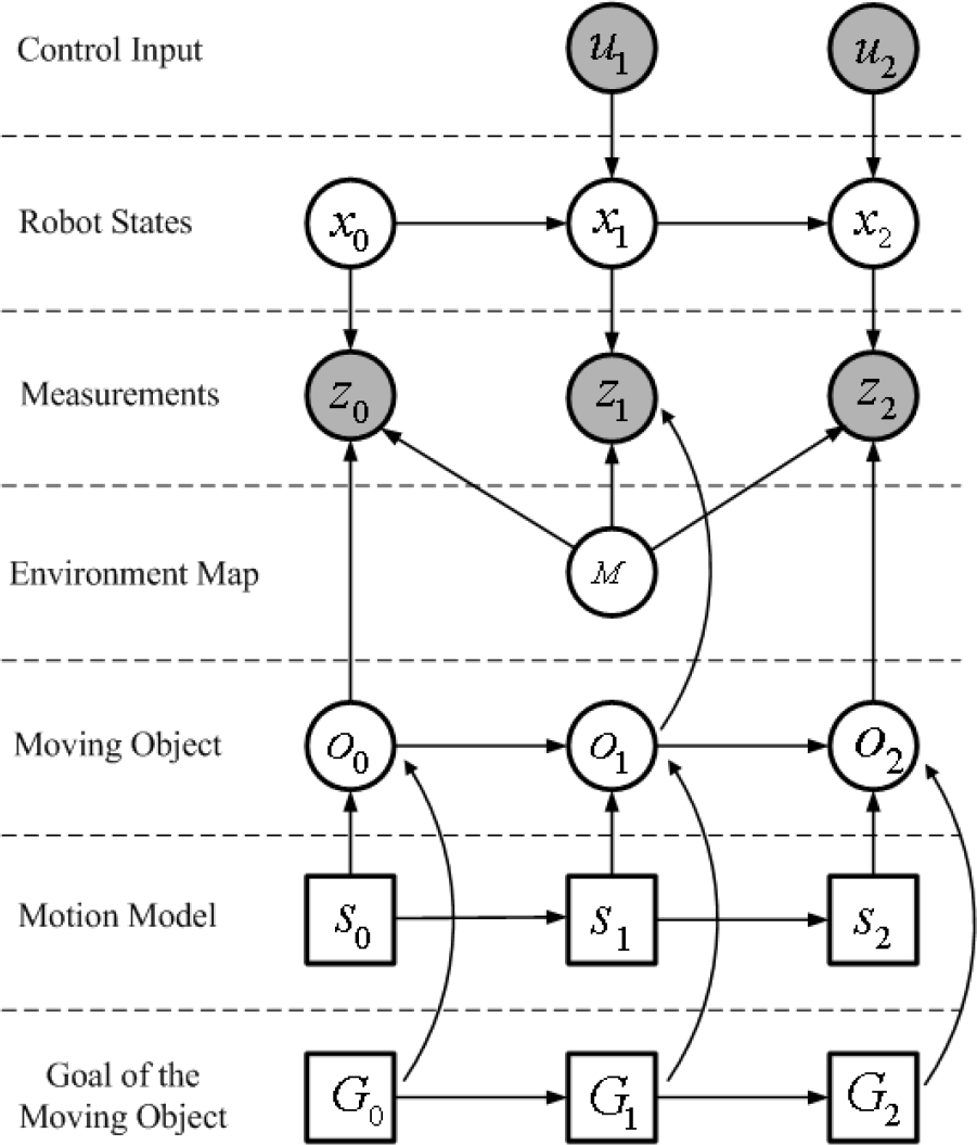
DBNs for localization and tracking problem

The localization is done by our previous works [7]. The detail is beyond the scope of this paper and will not be addressed here. Our focus will turn to the tracking formulation and further discuss the prediction framework.

3.1 Formulation of Tracking

The detection and tracking of moving object problem has been extensively studied for decades. To enhance tracking performance, it sometimes combines with prior motion models to predict the next states of moving objects. Considering the simplicity and efficiency, Kalman filter is commonly used in tracking problem. Recently, tracking over probability association is also the popular solution [3, 26].

We assume that the pedestrian motion is influenced by motion models and the intended goals. Accordingly, the prediction consists of short term and long term prediction. The short term prediction follows the motion model, such as constant velocity model and constant acceleration model etc., marked as s. In the long term prediction, the proposed pedestrian motion model is utilized. Moreover, in this paper, MHT (Multiple Hypothesis Tracking) is used to achieve robust data association.

Tracking problem can be treated as the posterior p(o_k | Z_k) estimation. According to the total probability and Bayesian formulation, the posterior is factorized into Eq. (12).

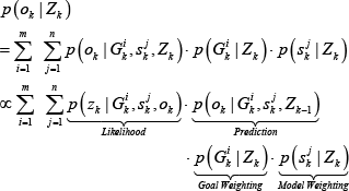
\begin{array}{l} p (o_{k}^{​} | Z_{k}^{​}) \\ = \sum_{i = 1}^{m} \sum_{j = 1}^{n} p (o_{k}^{​} | G_{k}^{i}, s_{k}^{j}, Z_{k}^{​}) \cdot p (G_{k}^{i} | Z_{k}^{​}) \cdot p (s_{k}^{i} | Z_{k}^{​}) \\ \propto \sum_{i = 1}^{m} \sum_{j = 1}^{n} \underset{L i k e l i h o o d}{\underset{︸}{p (z_{k}^{​} | G_{k}^{i}, s_{k}^{j}, o_{k}^{​})}} \cdot \underset{P r e d i c t i o n}{\underset{︸}{p (o_{k}^{​} | G_{k}^{i}, s_{k}^{j}, Z_{k - 1}^{​})}} \\ \cdot \underset{G o a l W e i g h t i n g}{\underset{︸}{p (G_{k}^{i} | Z_{k}^{​})}} \cdot \underset{M o d e l W e i g h t i n g}{\underset{︸}{p (s_{k}^{j} | Z_{k}^{​})}} \end{array}

(12)

p(z_k | Gⁱ_k, s^j_k, o_k) is the likelihood probability at time step k. The second term p(o_k| Gⁱ_k, s^j_k, Z_k-1) is the prediction process. Here, m and n indicate the number of goals and short term motion models. Motion model weighting p(s^j_k | Z_k) can also be factorized into Eq. (13).

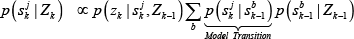
p (S_{k}^{j} | Z_{k}^{​}) \propto p (z_{k} | S_{k}^{j} Z_{k - 1}^{​}) \sum_{b} \underset{M o d e l T r a n s i t i o n}{\underset{︸}{p (S_{k}^{j} | S_{k - 1}^{b})}} p (S_{k - 1}^{b} | Z_{k - 1}^{​})

(13)

The third term p(Gⁱ_k | Z_k) of Eq. (12) represents the goal weighting. If we consider the uncertainty of sensor measurement and data association (tracking), the formula of goal weighting can be further divided into

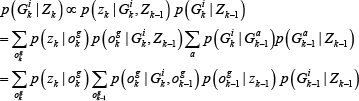
\begin{array}{l} p (G_{k}^{j} | Z_{k}^{​}) \propto p (z_{k} | G_{k}^{j}, Z_{k - 1}^{​}) p (G_{k}^{i} | Z_{k - 1}^{​}) \\ = \sum_{o_{k}^{g}} p (z_{k}^{​} | o_{k}^{g}) p (o_{k}^{g} | G_{k}^{i}, Z_{k - 1}^{​}) \sum_{a} p (G_{k}^{i} | G_{k - 1}^{a}) p (G_{k - 1}^{a} | Z_{k - 1}^{​}) \\ = \sum_{o_{k}^{g}} p (z_{k}^{​} | o_{k}^{g}) \sum_{o_{k - 1}^{g}} p (o_{k}^{g} | G_{k}^{i}, o_{k - 1}^{g}) p (o_{k - 1}^{g} | z_{k - 1}^{​}) p (G_{k - 1}^{i} | Z_{k - 1}^{​}) \end{array}

(14)

p(o^g_k | Gⁱ_k, o^g_k-1) is the proposed pedestrian prediction model. In this paper, we assume that the pedestrian does not change his goal. Thus, the probability p(Gⁱ_k | G^a_k-1) is equal to one if a is equal to i, and others are zero.

3.2 Formulation of Prediction

In prediction process, we split the problem into short term and long term prediction. Short term prediction forecasts the next status of the moving object which is directly influenced by motion models. Using the total probability, the short term prediction p(o_k+1 | o_k) can be rewritten as the combination of motion model p(o_k+1 | s^j_k, o_k) and model weighting p(s^j_k | o_k).

p (o_{k - 1}^{​} | o_{k}^{​}) = \sum_{j = 1}^{n} \underset{P r e d i c t i o n}{\underset{︸}{p (o_{k + 1}^{​} | s_{k}^{j}, o_{k})}} \underset{M o d e l W e i g h t i n g}{\underset{︸}{p (s_{k}^{j} | o_{k})}}

(15)

Notice that continuous state ok is used in short term prediction and EKF (Extended Kalman Filter) is utilized in this part. In long term prediction, the motion is directed by the intended goal. Considering the uncertainty of prediction, the motion in the N time step can be modeled as the combination of individual long term pedestrian models with different weights. Since long term prediction is based on grid space, prediction model p(o_k+N | o_k) is replaced by p(o^g_k+N | o^g_k). The formulation of long term prediction is derived as

\begin{array}{l} p (o_{k + N}^{g} | o_{k}^{g}) = \sum_{i}^{m} \underset{P r e d i c t i o n}{\underset{︸}{p (o_{k + N}^{g} | o_{k}^{j}, G_{k}^{i})}} \cdot p (G_{k}^{j} | o_{k}) \\ = \sum_{i}^{m} \underset{P r e d i c t i o n}{\underset{︸}{p (o_{k + N}^{g} | o_{k}^{j}, G_{k})}} \cdot \underset{G o a l W e i g h t i n g}{\underset{︸}{p (G_{k}^{j} | Z_{k})}} \end{array}

(16)

Since the term p(Gⁱ_k | o^g_k) inherently expresses goal weighting, p(Gⁱ_k | Z_k) is used in place of it and estimated by Eq. (14). The term p(o^g_k+N|o^g_k, Gⁱ_k) can be further estimated by Eq. (8). To demonstrate the prediction module, Figure 10 simulates the prediction results by observing sequential pedestrian motions.

Figure 10.

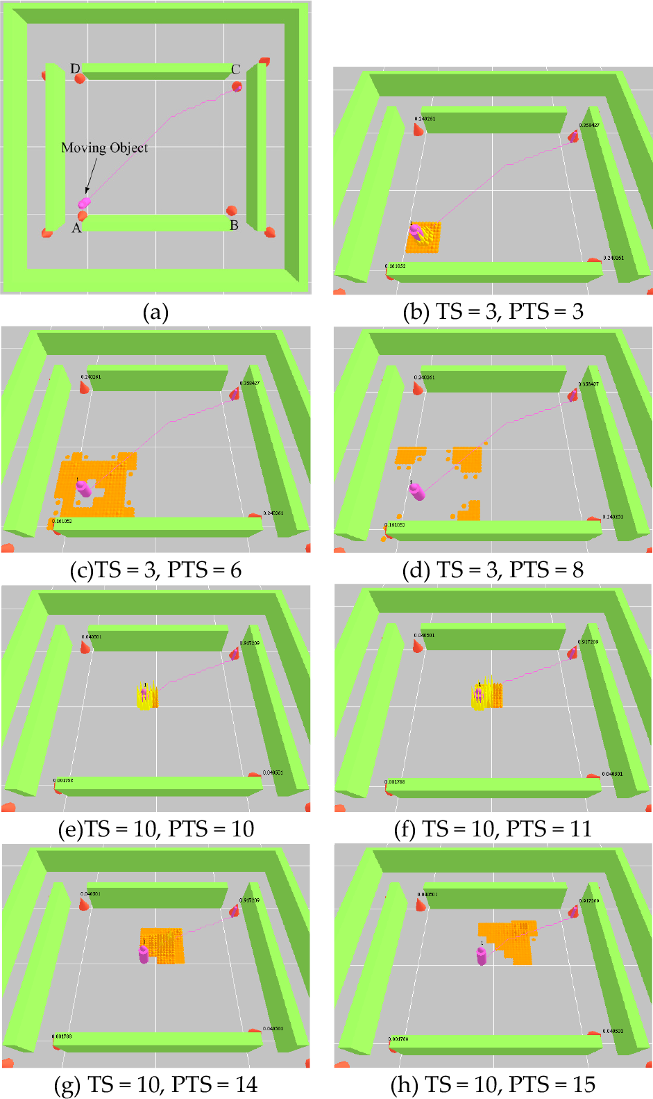
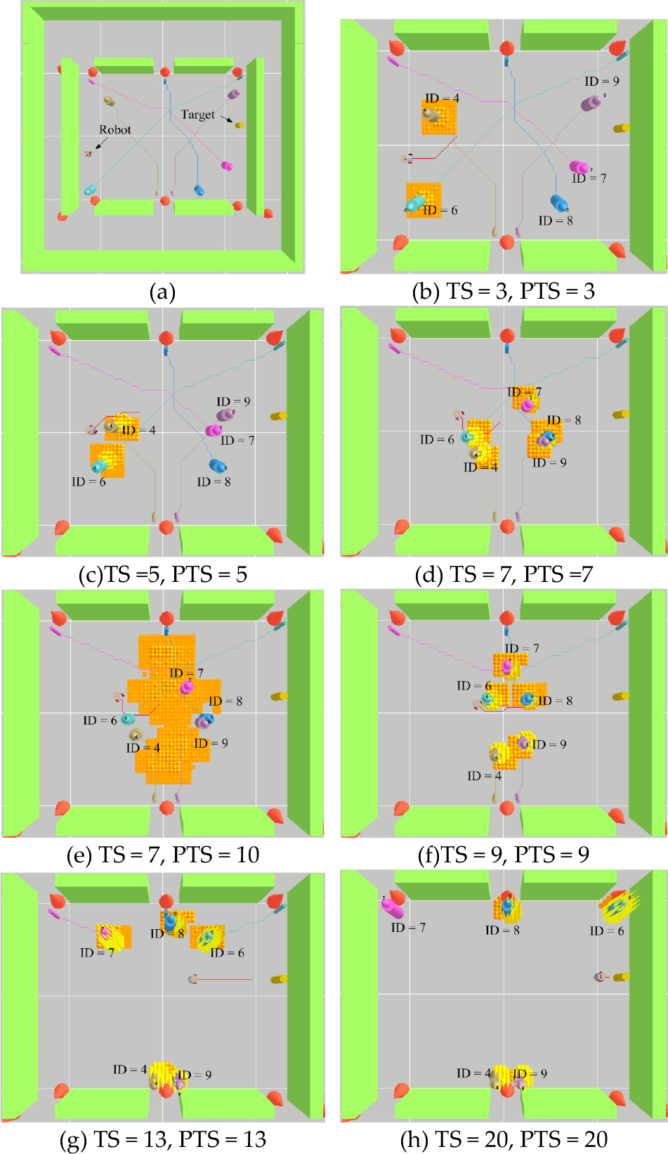
Motion prediction by the pedestrian model. TS and PTS indicate current time step and predicted time step

The simulation environment is displayed in Figure 10 (a). Four red cones marked as A to D are the potential goals of the pedestrian which are extracted from the GVG skeleton. The pedestrian moves from A to C. The simulated trajectory of the pedestrian is generated by A^* planner. Here TS and PTS of figure caption mean current time step and predicted time step. The height of the orange surface represents the occupied probability in predicted time step. The higher part of surface indicates higher occupied probability and its corresponding color will approach golden yellow. To simplify the description, we use the symbol p(A) to indicate the probability toward goal A.

The time axis of C-T Space in our planner is evaluated from current time step to the next ten seconds in every 0.5 second. Two time steps TS = 3 and TS = 10 are shown in Figure 10. In TS = 3, the estimated probability of potential goals from A to D is 0.16, 0.24, 0.35 and 0.24. Since the likelihood is almost equal, the predicted occupied areas will go toward four directions individually, as shown in Figure 10 (b)-(d). However, after a few seconds, the intention of the pedestrian is more obvious and p(C) increases rapidly. In TS = 10, the likelihoods of intended goals are 0.0017, 0.04, 0.917 and 0.04. The predicted occupied areas are merged into one large block toward goal C (Figure 10 (e)-(h)).

4. Predictive Anytime Planning

Real time motion planning is a very important and crucial constraint for mobile robots in dynamic environments. However, when the environment is complex, it may not be possible to obtain the optimal solution within the deliberation time. Anytime algorithms always keep a current best solution whatever the complete and optimal planning has been finished. Thus, the anytime framework is useful and appropriate in such complex planning problem. Due to these advantages, anytime planning currently becomes one of the most popular topics in robotics.

In this section, we combine A^* planner with prediction and tracking modules. Considering the time limitation, the planner follows the anytime framework. At the same time, the uncertainties of localization and measurement are represented as the cost of C-T Space. Finally, a predictive anytime A^* planner is developed to incrementally search the best trajectory in dynamic environments.

4.1 Configuration Time Space (C-T Space)

To efficiently and safely move in crowded dynamic environments, temporal information is useful for motion planning. It dramatically decreases the probability of collision by taking into account the motions of moving objects in time sequences. Accordingly, the proposed planning algorithm established on C-T Space can efficiently incorporate time sequence information.

However, because of the huge computation, it is impossible to real-time update entire C-T Space. In other words, it only updates the area close to the robot, called Active Region, and only the moving objects falling in the active region are concerned. To consider the uncertainty but still save the computation, the uncertainties of measurements and robot actions are represented as the cost in each grid of C-T Space. Different kinds of cost functions in the proposed planner will be discussed in the following.

(a) The Cost from Static Map

The cost from static map is introduced by the uncertainty of the robot pose. Currently, robot pose is estimated by localization module and represented as the Gaussian distribution. According to the uncertainty of robot pose, the static map can be treated as an occupancy grid map Occ_static. The static cost C_static is proportional to the occupancy probability of Occ_static.

C_{s t a t i c} \propto p (O c c_{s t a t i c} | x_{k}, M)

(17)

(b) The Cost from Dynamic Map

In a similar way, the moving objects in different time step t can be modeled as a dynamic map Occ_dynamic,t. The cost from the dynamic map C_dynamic,t is proportional to the occupancy probability of Occ_dynamic,t in each grid state.

C_{d y n a m i c, t} \propto p (O c c_{d y n a m i c, t} | o_{t}); t = k \dots k + N

(18)

(c) The Cost from Actions

Since the actions of the robot are not completely deterministic in the real world, the stochastic effect often leads to collision. Thus, in addition to static and dynamic cost, the uncertainty of robot action is also considered. Eq. (19) shows the formulation of one step cost C(x_k,u_k).

c (x_{k}, u_{k}) = C o s t (u_{k}) + \sum_{x_{k + 1}^{g}} V (x_{k + 1}^{g}) p (x_{k + 1}^{g} | x_{k}, u_{k})

(19)

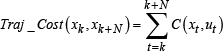
Here C_static(x) indicates the static cost of x and C_{dynamic, k+1}(x) expresses the dynamic cost of x at time step k+1. Finally, the total cost of a trajectory can be represented as the summation of all the step cost.

T a r j_C o s t (x_{k}, x_{K + N}) = \sum_{t = k}^{k + N} C (x_{t}, u_{t})

(20)

4.2 Predictive anytime A^* planner

To efficiently query a trajectory in C-T Space, an A^* based planner is adopted. Since our anytime planner only considers the local area close to the robot, it would be easily trapped in the “local minima”. To avoid this situation, a NF is utilized to guide the planner. In Figure 11 , we demonstrate the difference between Euclidean distance and NF in a spiral shape environment.

Figure 11.

spiral shape environment (a) environment map, (b) Euclidean distance easily causes local minima, (c) NF is the better distance description for navigation.

Moreover, NF is the key to make our planner follow the anytime framework. Using NF, the robot can query a suboptimal path very fast. NF is also a good indicator to measure the relative distance from current position to the goal and is utilized as the heuristic term in our A^* planner. In the beginning, an NF is only queried once from the goal to entire environment. Under anytime consideration, the current best trajectory is returned within the limited deliberation time. The criteria of trajectories are based on the total cost and heuristic term in the A^* planner. The current best trajectory will be the one that is the closest to the goal and the trajectory cost is below the threshold. The flowchart of our planner is shown in Figure 12 .

Figure 12.

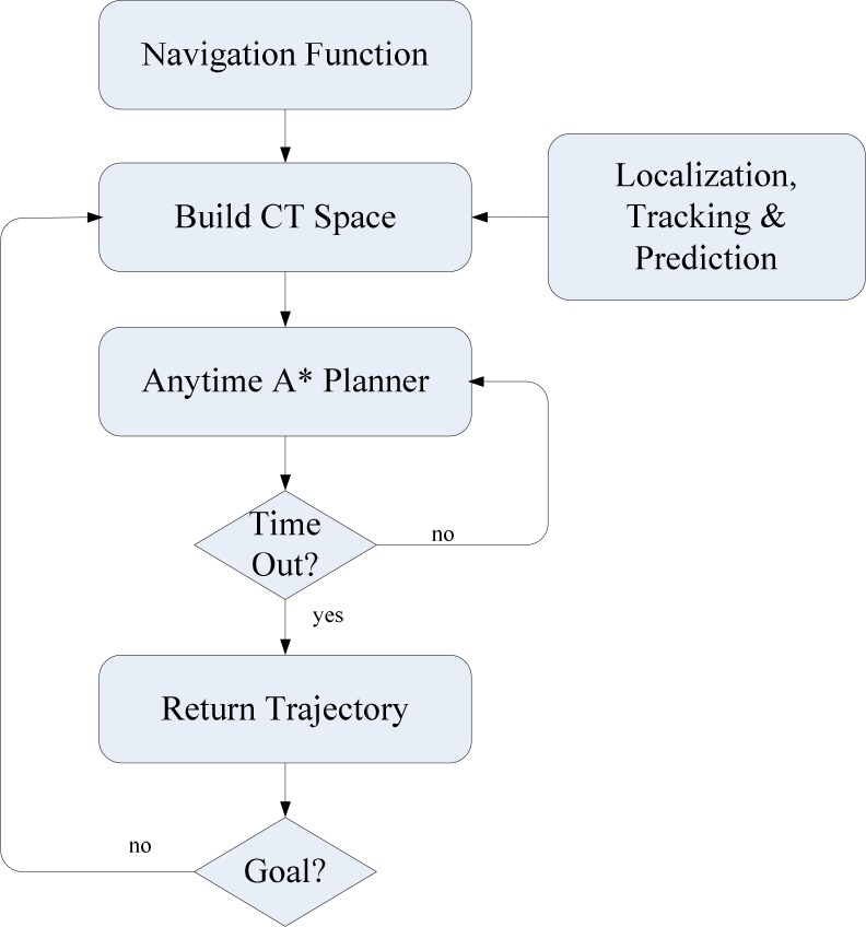
predictive anytime A^* planner

5. Simulations and Experiments

Simulations and experiments are shown in this section to verify the proposed idea. The simulation environment is contructed using C++ and OpenGL rendering engine. The hardware of the computer is Intel Core 2 Duo CPU and 2 GB RAM. In the experiments, environment map is built by the SLAM algorithms [7–8]. The deliberation time to query one trajectory is set to be 30ms. The robot, equipped with a laser range finder and two motor encoders, is shown in Figure 13 The demo video of simulations and experiments is available in the following internet address.

Figure 13.

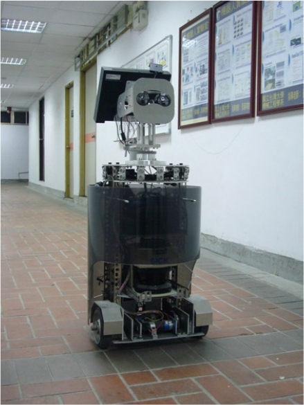
robot platform

http://www.youtube.com/watch?v=1Vmu9rI1Ah0

5.1 Simulation: Anytime Planning and Multiple Pedestrian Tracking

A crowded environment is simulated. Five pedestrians simultaneously move toward their goals. The simulated environment is displayed in Figure 14(a). There are six potential goals in this environment. In this simulation, the positions of pedestrian and robot are given but accompanied with Gaussian noise. Data association of moving objects is unknown. The robot is assigned to move from left side to right side. At the same time, it is required to track all the pedestrians. Deliberation time to query one trajectory is set to be 30ms in this simulation.

Figure 14.

Simulation II: crowded environment

Figure 14(b)-(h) show the simulation results in different time steps. Note that the robot chooses the trajectory at bottom side in TS = 7 (Figure 14(d)). The reason is that the bottom side area will get the lower collision cost in the next few seconds (Figure 14(e)). The simulation results demonstrate the robot can successfully pass through a crowded environment and the tracking results shown as tracking ID are corrected by comparing with ground truth.

5.2 Experiment I: Dynamic Obstacle Avoidance

In this experiment, the robot is required to perform navigation task and moving object avoidance. The map and estimated trajectories are shown in Figure 15. The details of anytime planning results are given in Figure 16 and Figure 17. The goals of the robot and the pedestrian are located in C and A.

Figure 15.

Exp.I - environment map.

Figure 16.

Exp.I- anytime planning and prediction

Figure 17.

Exp.I - Camera images in different time step

The scenario is described as follows. The robot reaches point 0 while the pedestrian is in the point1. However, by predicting the pedestrian motion in C-T Space, the robot realizes that the current steering direction will lead to collision. Thus, the anytime planner generates a more appropriate trajectory for collision avoidance (shown in Figure 16(a)). Figure 16(b)-(d) show the probability distribution of the predicted occupied area and corresponding predicted robot position. The camera images in Figure 17 demonstrate that the robot performs the real time obstacle avoidance after querying the trajectory. Figure 18 shows the estimated velocity of the pedestrian.

Figure 18.

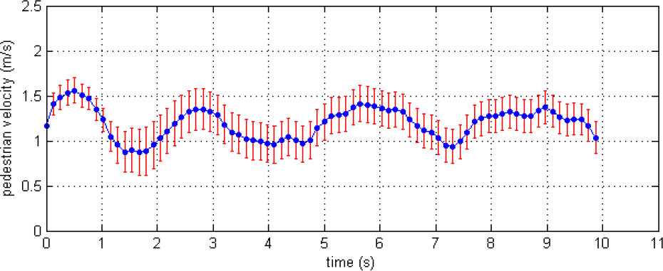
Exp.I - Estimated velocity of the pedestrian

In addition, the robot changes its steering direction even though the pedestrian is not really close to it yet. Thus, pedestrian is not blocked by the robot or compelled to slow down. In contrast to a reactive planner, the robot usually stops in the front of pedestrians and slowly moves along the shape of pedestrians for obstacle avoidance. The pedestrian needs to wait until the robot passes. Therefore, a predictive planner not only can decrease the probability of collision, but also efficiently shorten the navigation period

5.3 Experiment II: Compliant Motion

In experiment II, the environment consists of a narrow corridor and several rooms. The width of corridor is limited and is only capable of one pedestrian at one time. The environment map is shown in Figure 19. Four potential goals marked as A, B, C, and D are extracted. The goal of the pedestrian is located at D. The estimated trajectories of the robot and pedestrian are represented in Figure 20. The details are demonstrated in Figure 21. At first, since p(C) and p(D) are high, the robot comprehends that it may collide with the pedestrian. As a result, the planner generates a trajectory toward the waiting point and chooses to stay there until the pedestrian passes through the corridor. To emphasize the effect of prediction, we also compare it with a reactive planner. Five experiment trials under similar conditions are done for each planner. The statistical results of travel distance and period are shown in Figure 22 . Since the trajectory generated by the reactive planner easily blocks the pedestrian, the robot is often compelled to move back. As a result, the predictive planner gets shorter travel distance and period than the reactive planner does.

Figure 19.

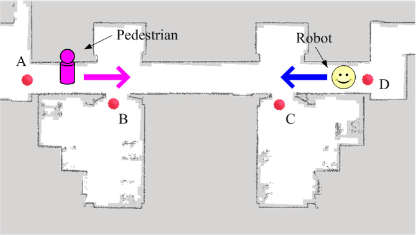
Exp.II - environment map.

Figure 20.

Exp.II - the trajectories of robot and pedestrian

Figure 21.

Exp.II (a) the robot observes the pedestrian and predicts potential locations of the pedestrian. The current time step is at 5 s and predicted time step is at 12 s. The corresponding camera image at time step 5 s is shown in right image. (b) the robot stays at the waiting point. (c) After the pedestrian passes, the robot keeps executing the navigation task

Figure 22.

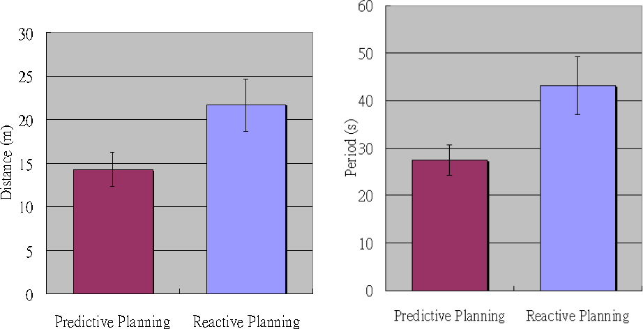
Predictive planning and reactive planning

6. Conclusions

In this paper, we proposed a predictive navigation planner for a mobile robot in populated environments. A generalized pedestrian model was represented and trained by analyzing the pedestrian trajectories. The pedestrian model can be applied to any similar environments without recollecting pedestrian trajectories. According to the pedestrian model, the robot is able to understand pedestrian intentions and further predict their motions. The unusual trajectories are also detected with this pedestrian model. By incorporating prediction and anytime framework in the planner, the robot can efficiently query trajectories in C-T Space. Moreover, in order to execute tasks in partially observable environments, a DBNs framework for localization, tracking and prediction is derived. Simulations and experiments show that the proposed planner efficiently tracks and predicts the possible occupied areas of moving objects in complex and dynamic environments. Finally, in the narrow corridor case, the robot is capable of performing the compliant motion to avoid the potential collision. The statistical results show that the proposed predictive planner gets better performance than a reactive one.

References

Aoyama

Ishikawa

Seki

Okamura

Ishimura

, and Satsumi

, “Development of mine detection robot system,” Int. J. of Advanced Robotic Systems, vol. 4, pp. 229–236, 2007.

Bennewitz

Burgard

Cielniak

, and Thrun

, “Learning Motion Patterns of People for Compliant Robot Motion,” Int. J. Robotics Research, vol. 24, pp. 31–48, 2005.

Blackman

S. S.

, “Multiple hypothesis tracking for multiple target tracking,” IEEE Aerospace and Electronic Systems Magazine, vol. 19, pp. 5–18, 2004.

Bohnert

Zukerman

Berkovsky

Baldwin

, and Sonenberg

, “Using interest and transition models to predict visitor locations in museums,” AI Communications, vol. 21, pp. 195–202, 2008.

Carreira

Canas

Silva

, and Cardeira

C. A. C. C.

, “i-Merc: A Mobile Robot to Deliver Meals inside Health Services,” Proc. IEEE Int. Conf. on Robotics, Automation and Mechatronics, Bangkok, Thailand, pp. 1–8, 2006.

Choset

and Burdick

, “Sensor based planning. I. The generalized Voronoi graph,” Proc. IEEE Int. Conf. on Robotics and Automation, Nagoya, Japan, vol. 2, pp. 1649–1655 1995.

Chung

S. Y.

and Huang

H. P.

, “Relative-Absolute information for simultaneous localization and mapping,” Proc. IEEE Int. Conf. on Robotics and Biomimetics, Sanya, China, pp. 1641–1646, 2007.

Chung

S. Y.

and Huang

H. P.

, “SLAMMOT-SP: Simultaneous SLAMMOT and Scene Prediction,” Advanced Robotics, vol. 24, pp. 979–1002, 2010.

Djekoune

A. O.

Achour

, and Toum

, “A sensor based navigation algorithm for a mobile robot using the DVFF approach,” Int. J. of Advanced Robotic Systems, vol. 6, pp. 97–108, 2009.

10.

Ellis

Sommerlade

, and Reid

, “Modelling Pedestrian Trajectories with Gaussian Processes,” 9th Int. Workshop on Visual Surveillance, Kyoto, Japan, 2009.

11.

Foka

and Trahanias

, “Real-time hierarchical POMDPs for autonomous robot navigation,” Robotics and Autonomous Systems, vol. 55, pp. 561–571, 2007.

12.

Foka

A. F.

and Trahanias

P. E.

, “Predictive autonomous robot navigation,” Proc. IEEE/RSJ Int. Conf. on Intelligent Robots and System, EPFL, Switzerland, vol. 1, pp. 490–495, 2002.

13.

Graf

Hans

, and Schraft

R. D.

, “Care-O-bot II - Development of a Next Generation Robotic Home Assistant,” Autonomous Robots, vol. 16, pp. 193–205, 2004.

14.

Hansen

E. A.

and Zhou

, “Anytime heuristic search,” J. Artificial Intelligence Research, vol. 28, pp. 267–297, 2007.

15.

Chia-Hung

H. Harry

and Liu

, “A Flexible Architecture for Navigation Control of a Mobile Robot,” IEEE Trans. on Systems, Man and Cybernetics, Part A: Systems and Humans, vol. 37, pp. 310–318, 2007.

16.

Izumi

Habib

M. K.

Watanabe

, and Sato

, “Behavior selection based navigation and obstacle avoidance approach using visual and ultrasonic sensory information for quadruped robots,” Int. J. of Advanced Robotic Systems, vol. 5, pp. 379–388, 2008.

17.

Kanda

Glas

D. F.

Shiomi

M. F.

, and Hagita

N. F.

, “Abstracting People's Trajectories for Social Robots to Proactively Approach Customers,” IEEE Trans. on Robotics, vol. 25, pp. 1382–1396, 2009.

18.

Koenig

and Likhachev

, “Fast replanning for navigation in unknown terrain,” IEEE Trans. on Robotics, vol. 21, pp. 354–363, 2005.

19.

Likhachev

Ferguson

Gordon

Stentz

, and Thrun

, “Anytime search in dynamic graphs,” Artificial Intelligence, vol. 172, pp. 1613–1643, 2008.

20.

Nakauchi

and Simmons

, “A social robot that stands in line,” Autonomous Robots, vol. 12, pp. 313–324, 2002.

21.

Pacchierotti

Christensen

H. I.

, and Jensfelt

, “Evaluation of Passing Distance for Social Robots,” Proc. The 15th IEEE Int. Sym. on Robot and Human Interactive Communication, Hatfield, UK, pp. 315–320, 2006.

22.

Pineau

Gordon

, and Thrun

, “Point-based value iteration: An anytime algorithm for POMDPs,” Proc. Int. Conf. on Artificial Intelligence, Acapulco, Mexico, pp. 1025–1032, 2003.

23.

Poncela

Urdiales

Perez

E. J.

, and Sandoval

, “A new efficiency-weighted strategy for continuous human/robot cooperation in navigation,” IEEE Trans. on Systems, Man, and Cybernetics Part A: Systems and Humans, vol. 39, pp. 486–500, 2009.

24.

Sakamoto

Honda

Inami

, and Igarashi

, “Sketch and Run: A Stroke-based Interface for Home Robots,” Proc. 27th Annual SIGCHI Conf. on Human Factors in Computing Systems, Boston, USA, pp. 197–200, 2009.

25.

Satake

Kanda

Glas

D. F.

Imai

Ishiguro

, and Hagita

, “How to approach humans?: strategies for social robots to initiate interaction” Proc. ACM/IEEE Int. Conf. on Human-Robot Interaction, La Jolla, CA, USA, pp. 109–116 2009.

26.

Schulz

Burgard

Fox

, and Cremers

A. B.

, “People Tracking with Mobile Robots Using Sample-Based Joint Probabilistic Data Association Filters,” Int. J. Robotics Research, vol. 22, pp. 99–116, 2003.

27.

Shiomi

Kanda

Ishiguro

, and Hagita

, “Interactive humanoid robots for a science museum,” IEEE Intelligent Systems, vol. 22, pp. 25–32, 2007.

28.

Sisbot

E. A.

Marin-Urias

L. F.

Alami

, and Simeon

, “A Human Aware Mobile Robot Motion Planner,” IEEE Trans. on Robotics, vol. 23, pp. 874–883, 2007.

29.

Stentz

, “The Focussed D Algorithm for Real-Time Replanning.,” Proc. Int. Conf. on Artificial Intelligence, Montreal, Quebec, Canada, pp. 1652–1659, 1995.

30.

Stutters

Honghai

Tiltman

, and Brown

D. J.

, “Navigation Technologies for Autonomous Underwater Vehicles,” IEEE Trans. on Systems, Man, and Cybernetics, Part C: Applications and Reviews, vol. 38, pp. 581–589, 2008.

31.

Thrun

, “Learning Metric-Topological Maps for Indoor Mobile Robot Navigation,” Artificial Intelligence, vol. 99, pp. 21–71, 1998.

32.

Thrun

Beetz

Bennewitz

Burgard

Cremers

A. B.

Dellaert

Fox

Hahnel

Rosenberg

Roy

Schulte

, and Schulz

, “Probabilistic algorithms and the interactive museum tour-guide robot Minerva,” Int. J. of Robotics Research, vol. 19, pp. 972–999, 2000.

33.

Wagner

A. R.

, “Creating and using matrix representations of social interaction,” Proc. 4th ACM/IEEE Int. Conf. on Human Robot Interaction, La Jolla, CA, USA, pp. 125–132, 2009.

34.

Yen

H. C.

Huang

H. P.

, and Chung

S. Y.

, “Goal-Directed Pedestrian Model for Long-Term Motion Prediction with Application to Robot Motion Planning,” Proc. IEEE Int. Conf. on Advanced Robotics and its Social Impacts, Taipei, Taiwan, pp. 1–6, 2008.

35.

Yoon

Roh

K. S.

, and Shim

, “Vision-based obstacle detection and avoidance: Application to robust indoor navigation of mobile robots,” Advanced Robotics, vol. 22, pp. 477–492, 2008.

36.

Zhang

Liu

, and Zong

, “Mechanical design and dynamcis of an autonomous climbing robot for elliptic half-shell cleaning,” Int. J. of Advanced Robotic Systems, vol. 4, pp. 437–446, 2007.

37.

Zhou

Tan

Cao

Wang

, and Wang

, “The design and implementation of a biomimetic robot fish,” Int. J. Advanced Robotic Systems, vol. 5, pp. 185–192, 2008.

38.

Zucker

Kuffner

, and Branicky

, “Multipartite RRTs for rapid replanning in dynamic environments,” Proc. IEEE Int. Conf. on Robotics and Automation, Rome, Italy, pp. 1603–1609, 2007.

Predictive Navigation by Understanding Human Motion Patterns

Abstract

Keywords

1. Introduction

2. Pedestrian Model Learning

2.1 Potential Goal Extraction

2.2 Generalized Pedestrian Motion Model

2.3 Pedestrian Model Learning

(a) Motion Model in DistMap

(b) Motion Model in NF

(c) Pedestrian Model Evaluation

(d) Motion Prediction

3. Probabilistic Framework

3.1 Formulation of Tracking

3.2 Formulation of Prediction

4. Predictive Anytime Planning

4.1 Configuration Time Space (C-T Space)

(a) The Cost from Static Map

(b) The Cost from Dynamic Map

(c) The Cost from Actions

4.2 Predictive anytime A* planner

5. Simulations and Experiments

5.1 Simulation: Anytime Planning and Multiple Pedestrian Tracking

5.2 Experiment I: Dynamic Obstacle Avoidance

5.3 Experiment II: Compliant Motion

6. Conclusions

References

4.2 Predictive anytime A^* planner