Sage Journals: Discover world-class research

Abstract

Currently, the main component of most U.S. consumers’ electricity bills is based on a constant price per kWh consumed. As intermittent renewable resources and flexible loads that can be shifted within days (such as electric vehicle charging) gain prominence in the electricity system, the efficiency gains to be realized from basing bills instead on wholesale spot prices increase. There is little political support for this change, however. We focus on second-best alternatives: time-of-use (TOU) rates and critical peak pricing (CPP). We introduce alternative assessment criteria that focus on intra-day load shifting. Using historical data, we find that TOU rates can reasonably replicate the intra-day load-shifting incentives provided under spot pricing. Thus, TOU rates, especially when complemented with CPP involving load control during infrequent scarcity price events, can be considerably more socially valuable than previously estimated.

Keywords

Electricity Retail Rates Electricity Markets Demand Response Renewables

1. Introduction

Currently, in the U.S., only a relatively small number of large commercial and industrial consumers are active in wholesale energy markets, typically through arrangements with wholesale intermediaries. These consumers can respond to variations in short-term prices by adjusting their consumption and have experience using hedging strategies to manage the risks of price variations on bill stability. For most end users, however, the interface between the supply and demand side is the retail rate offered by load-serving entities (LSE), either traditional distribution companies offering bundled delivery and energy services or competitive retailers offering unbundled energy services. Traditionally, electricity retail rates for residential and small commercial consumers have been mostly flat, i.e., a relatively small customer charge plus a price per kWh consumed. The per kWh rate is often constant for no less than a year and often much longer.¹ The rate reflects the recent historical or expected average cost of energy and delivery costs, which are mainly fixed in the short run.² Flat rates have often been criticized for their failure to reflect “peak load pricing” considerations either ex-ante or in real time, resulting in inefficient consumption and investment (Borenstein and Holland, 2005; Joskow and Wolfram, 2012).

Developments on both the supply and demand sides of wholesale markets have led to an increased importance of retail rate designs that better reflect variations in wholesale energy prices. On the supply side, the share of intermittent renewable generation in the power mix is rising in many countries. This change in the supply mix leads to more volatile power prices, more hours of very low prices, more hours of high prices and scarcity conditions, and thus more value that can be derived from demand-side flexibility in the short and long run (Vijay et al., 2017; Ekholm and Virasjoki, 2020; Mallapragada et al., 2021; Imelda et al., 2022). On the demand side, opportunities for end-users to better manage their load are expanding, enabled by digitalization and the adoption of electric vehicles, heat pumps, stationary batteries, and other controllable loads (BNEF, 2022; IEA, 2021). To some extent, these loads can be programmed in advance to react to time-varying prices observed via smart meters or load control arrangements with LSEs.

This paper focuses on how to better reflect the time-varying conditions in the wholesale electricity markets in residential and small commercial retail rates while balancing consumer preference for price predictability and bill stability. It has long been argued that it would be optimal to charge end-users wholesale spot prices for energy, often termed dynamic pricing or real-time pricing (RTP) (Schweppe et al., 1988).³ However, the adoption of retail rates that vary with spot wholesale prices has lagged far behind the deployment of smart meters with the necessary capabilities in the U.S.⁴ In practice, even though dynamic pricing is technically feasible, small consumers generally prefer predictability and bill stability. Frequently reacting to price information might be more costly than the potential benefits-rational inattention-and consumers are risk-averse as they want to avoid large, unexpected upswings in their bill. The occurrence of periods of sustained high prices, in particular, besides creating consumer acceptability issues, also leads to political turmoil, as evidenced by the Texas energy crisis in February 2021 (Littlechild and Kiesling, 2021) and the European energy crisis that has been ongoing since the summer of 2021 (Batlle et al., 2022a). These two barriers to the adoption of spot pricing are not unsurmountable; a lack of predictability can be mitigated by introducing a high degree of automation in electricity consumption, and bill stability can be guaranteed by complementing dynamic pricing with a hedge or insurance product. However, they are not expected to be reduced significantly in the next years, at least not for a large share of the population.

Trabish (2022) reports that there were over 150 rate design initiatives in 2021 addressing new forms of time-varying rates in the U.S., typically acting as a sort of intermediary between flat and hourly dynamic pricing. Many of these are pilot programs. We focus on two popular rate designs of this sort: time-of-use rates (TOU) and critical peak pricing (CPP). TOU rates are predefined, e.g., at least a year ahead, and calibrated on historical price data. Typically, the TOU rate coefficients differ by season, type of day (workdays or weekends), and/or time of the day (e.g., peak, shoulder, or off-peak). Under TOU rates, consumers are given predictable incentives to shift or reduce their demands and are protected from unexpected price shocks.⁵ Faruqui et al. (2020) report that nearly 400 TOU rates have been tested in pilots globally. Opt-in TOU rates are increasingly available, which may result in adverse selection issues (Qiu et al., 2017), but uptake is typically limited. More recently, several state regulators, notably those in California and Hawaii, have adopted default TOU rates from which consumers may opt out (Kavulla, 2023).

Different from TOU rates, CPP is designed to induce reductions in consumption, either through demand shifting or conservation during hours with the highest wholesale prices, often associated with the highest net demand days of the year.⁶ The system operator announces CPP events on a short notice, e.g., day-ahead—see e.g., Herter (2007). During a critical peak pricing event, a consumer enrolled in a CPP plan is then exposed to a significantly increased price for the duration of the event (typically not more than a few hours). An alternative or additional feature is for consumers to allow for remote load control during critical peak pricing events. In exchange for their consent, consumers receive a discount on their electricity bill. Consumers can typically override the load control but often at the expense of their bill discount or a penalty. The maximum number of peak events that the system operator can trigger per season or year is predefined. Examples are the Peak Day Pricing plan offered by PG&E (2022) in California and the load management pilot offered by Xcel Energy (2022) in Texas for commercial consumers.

We compute four criteria for assessing the performance of alternative retail rate designs compared to the status quo, flat rates, and the first-best benchmark, dynamic pricing. The four criteria can be divided into two groups: time series analysis and simulation models. For each group, we use one criterion that has been commonly applied in the existing literature (see Section 2 below) and we contrast the results with one novel criterion, which we argue is more appropriate in a context with increasing volumes of load that can be shifted with relative ease within a day. With regards to the time series analysis, in addition to the computation of the annual (standard) Pearson correlation between spot prices and the alternative rates, as relied upon in the previous literature, we introduce the use of the daily Spearman rank correlation between spot prices and the alternative rates to better reflect incentives to shift consumption between hours of the day. The Pearson correlations reflect absolute wholesale prices variations over time while the Spearman rank correlations reflect relative wholesale price variations between hours within a day. High Spearman rank correlations mean that TOU pricing gives load-shifting incentives that are directionally correct. The two simulation models permit a more detailed analysis of the replication of load-shifting incentives of TOU rates compared to dynamic pricing, assuming full consumer response. In addition to representing load with independent hourly demand functions, as in the prior literature, we model load shifting with a new cost-minimizing optimization model in which shiftable loads are characterized by the minimum anticipation and maximum delay in their electricity consumption relative to a baseline schedule and a constant cost per kWh shifted. We present illustrative cost calculations for different TOU rate designs, complemented or not by CPP. The TOU rates for a particular year are calibrated based on the preceding three years of wholesale prices. CPP is proxied by the replacement of the TOU rates by the observed wholesale price for a limited number of the highest priced hours per year.

We compute the criteria using data from three US power systems for a period between 2011-2020: the systems operated by the Electric Reliability Council of Texas (ERCOT), the California Independent System Operator (CAISO) and the Independent System Operator of New England (ISO-NE). ERCOT has a high wind penetration, with 23% of electricity produced by wind in 2020 (ERCOT, 2021). Wind plus solar PV accounted for about 25% of generation in 2020. CAISO has a high penetration of grid-based solar PV; 22% of electricity was generated by solar PV in 2020. Grid-based solar PV plus wind accounted for about 28% of the generation (California Energy Commission, 2022). ISO-NE is gas-dominated system without significant penetration of grid-based intermittent renewables; only about 5% of electricity generation came from wind and grid-based solar PV combined in 2020 (ISO-NE, 2022a). We can think of ISO-NE as a control representing the thermal-dominated systems upon which many of the previous papers relied.⁷

The remainder of the paper is organized in six sections. In Section 2, we discuss the existing literature and our contribution. In Section 3, we introduce the different criteria to evaluate retail rate design. In Section 4, we describe the data and the process to calibrate the TOU rates. In Section 5, we present the results. In Section 6, we provide a discussion. Finally, we present a conclusion and policy recommendations.

2. The Existing Literature and Our Contribution

First, we describe the existing relevant literature. Afterwards, we highlight our contribution.

2.1 Existing Literature on Alternative Time-varying Rate Designs

Time-varying electricity retail rates are not a recent idea. Hausman and Neufeld (1984) explain that electricity rates with varying price levels over the course of the day were already discussed around the turn of the last century when the electricity industry was still in its infancy. However, since then attempts to introduce them have largely been unsuccessful. A major breakthrough in the academic literature was the seminal work of Boiteux (1949) to whom the practical application of marginal cost pricing to electricity is ascribed. Boiteux elaborated upon the concept of peak-load pricing, which implies that an efficient schedule of prices consists of a tariff that is set equal to system marginal running cost when there is idle capacity (i.e., off-peak periods), and equal to long run marginal cost in peak periods. The peak-pricing concept was later further elaborated upon by Steiner (1957), Turvey (1968) and others. A discussion of the different contributions to the theory of marginal cost pricing applied to electricity is provided by Joskow (1976). Later, Schweppe et al. (1988) formulated the theory of dynamic pricing that respects the particular conditions of electric power transmission systems.

More recently, two literature streams on time-varying retail rates for electricity have been developing: the analysis of consumer response to time-varying retail rates and the analysis of the extent to which different approaches to time-varying retail rates can approximate the incentives provided under wholesale spot prices. Most of the research on time-varying retail rates has focused on how consumers respond to such rates. Faruqui and Sergici (2013) provide an extensive survey of global experience with time-varying rates, reviewing the results of 34 studies encompassing 163 experimental treatments in four continents and seven countries. They argue that there is a surprising amount of consistency in the results of all these studies, which shows that utilities and policymakers can be confident that time-varying prices, such as TOU rates, will yield significant peak-load reductions. Some studies, e.g., Liang et al. (2020), also specifically focused on how time-varying rates impact consumer decisions with regards to the adoption of energy efficient appliances and distributed energy resources such as solar PV.

Less research has investigated how well different time-varying rates replicate the incentives for load shifting that would occur under dynamic pricing, i.e., the quality of the approximation. We focus on that question. The few available studies of that question have concluded that TOU rates only capture a small fraction, often about one-fifth or less, of the welfare benefits from dynamic pricing (Borenstein, 2005; Holland and Mansur, 2006; Spees and Lave, 2008; Hogan, 2014; Jacobsen et al., 2020). These authors use three types of approaches: computation of correlations between spot prices and TOU rates, simulation models computing short-run welfare from TOU rates versus dynamic pricing, and simulation models computing long-run welfare effects of alternative rates (including capacity investment on the supply side). By coincidence, all of these papers use data from the Pennsylvania-New Jersey-Maryland (PJM) Interconnection, with the exception of Borenstein (2005), who builds his own simulation model. During the time periods covered in these studies, PJM was a predominantly thermal system with little wind and solar generation.

Hogan (2014) and Jacobsen et al. (2020) use the first approach, i.e., the computation of correlations between spot prices and TOU rates. They compute the R2 from a regression of observed wholesale prices on season, day of week, or within-day price periods (which vary according to the exact TOU rate design). The reasoning is that the expected deadweight loss from applying TOU rates is proportional to the residual variance of the deviations between the TOU rates and spot prices. Hogan (2014) considers the case in which each hour’s demand curve is linear with the same slope but a shifting intercept. He finds for 2013 data that only 23% of the benefit of going from flat rates to dynamic pricing is captured using TOU pricing. Jacobsen et al. (2020) formalize a more general analytical framework and use 2012 data to compute the in-sample yearly correlation for seven alternative TOU rates. The highest in-sample R2 value they find is 0.428 for their most complicated TOU rate (hour x day of week x month scheme). The same authors also confirm these results by a simulation. Holland and Mansur (2006) and Spees and Lave (2008) estimate the short-run welfare effects of TOU rates versus dynamic pricing using a simulation model. Holland and Mansur (2006) find a range of 15% to 30% of short-run welfare benefits for different TOU rates compared to dynamic pricing simulated for the period April 1998 to March 2000. Spees and Lave (2008), using 2006 data, find that peak capacity savings are seven times larger with dynamic pricing. Finally, Borenstein (2005) introduces a simulation model with three generation technologies to compute the long-run welfare gains of TOU rates versus dynamic pricing. He computes that, roughly speaking, TOU rates capture 20% of the efficiency gains.

2.2 Our Contribution

We modify two crucial assumptions in the literature just discussed: the characterization of demand-side flexibility and of the generation mix of the power system considered.

Regarding the characterization of demand-side flexibility, both the approach looking at the R2 between dynamic pricing and TOU rates and the different types of simulation models implicitly or explicitly consider independent hour-specific demand functions for electricity. Aside from criticalpeak periods, in which load may be mainly reduced, not shifted, we think that demand shifting is the more important short-run response. This trend has been recognized by practitioners (see e.g., CPUC (2022)) but mostly disregarded by the academic literature. Especially at the household level, a large fraction of demand flexibility is expected to come from frequent within-day “load shifting”, or “appliance scheduling” when considering the important and accelerating trend of electrification of HVAC and transport (Borlaug et al., 2020; Zhou et al., 2022). Some shifting can be programed in advance or just embodied in habits (e.g., “charge the EV at noon whenever possible”) to respond to predictable TOU rates. Frequent within-day load shifting has very different properties than electricity consumption represented by independent hour-specific demand functions. More precisely, when considering the case of within-day load shifting, relative price differences between hours, or groups of adjacent hours, are more important than absolute price differences between individual hours.

Regarding the characterization of the supply side, we note that essentially almost all the studies in the surveyed literature were performed before there was significant penetration of intermittent wind and solar generation. That is, they reflected wholesale price variations for primarily thermal systems. This does not reflect either the present or, more importantly, the future as electric power systems decarbonize. As wind and solar penetration increases, wholesale price distributions will change dramatically with many more zero or very low-price hours and many more high-price and scarcity hours (Mallapragada et al., 2021). These changing wholesale price distributions, along with the increasing penetration of within-day shiftable loads, are likely to change the net social benefits of incentivizing within-day load shifting.

Further, in the proposed framework for analysis, we also want to estimate the additional impact of complementing TOU rates with a CPP program. While frequent load shifting is becoming more important and should be considered when assessing alternative rate designs, a crucial driver of the value of flexibility in electricity consumption remains demand reductions during infrequent scarcity conditions. TOU rates are not dynamic enough to capture these infrequent scarcity events. As a result, any time-varying rate would benefit from the addition of a CPP program, especially a program entailing load control. Blonz (2022), applying a capacity expansion model calibrated on data from the North Californian PG&E service territory, estimates that a well-targeted peak pricing program could capture 83% of the savings relative to dynamic pricing.⁸ Mays and Klabjan (2017) emphasize the important role of CPP in reducing capacity costs.

3. Criteria to Evaluate Time-Varying Retail Rates

Section 3.1 describes the criteria based on the time series analysis. Section 3.2 introduces the simulation models with different representations of demand.

3.1 Time Series Analysis: Annual Pearson Correlation and Daily Spearman Rank Correlation

Hogan (2014) and Jacobsen et al. (2020) compute the R2 from a regression of observed hourly day-ahead spot prices on season, day of week, or within-day price periods (which vary according to the exact TOU rate design). Both calculate the in-sample R2 between a time series of TOU rates and day-ahead prices from PJM. In line with the existing literature, the first criterion that we compute is the annual Pearson correlation of spot prices and the TOU rates. The main difference being that we compute the out-of-sample correlation, rather than the in-sample R2. By out-of-sample we mean that the TOU rates are calibrated based on day-ahead hourly price data from the three preceding years, not from the observed year, corresponding roughly to current ratemaking practice. Section 4 provides more information.

As the annual Pearson correlation is strongly driven by scarcity price events, we also compute the annual Pearson correlation between the spot prices and the same TOU rate but with the ten highest observed priced hours in the spot market replacing the respective TOU rate during those hours. This rate design can be interpreted as TOU rates complemented with centralized load control under CPP. Figure 1 shows an annual time series of spot prices, i.e., the day-ahead prices for the CAISO SP15 Hub, a TOU rate calibrated based on historical prices, and CPP hours.

Figure 1

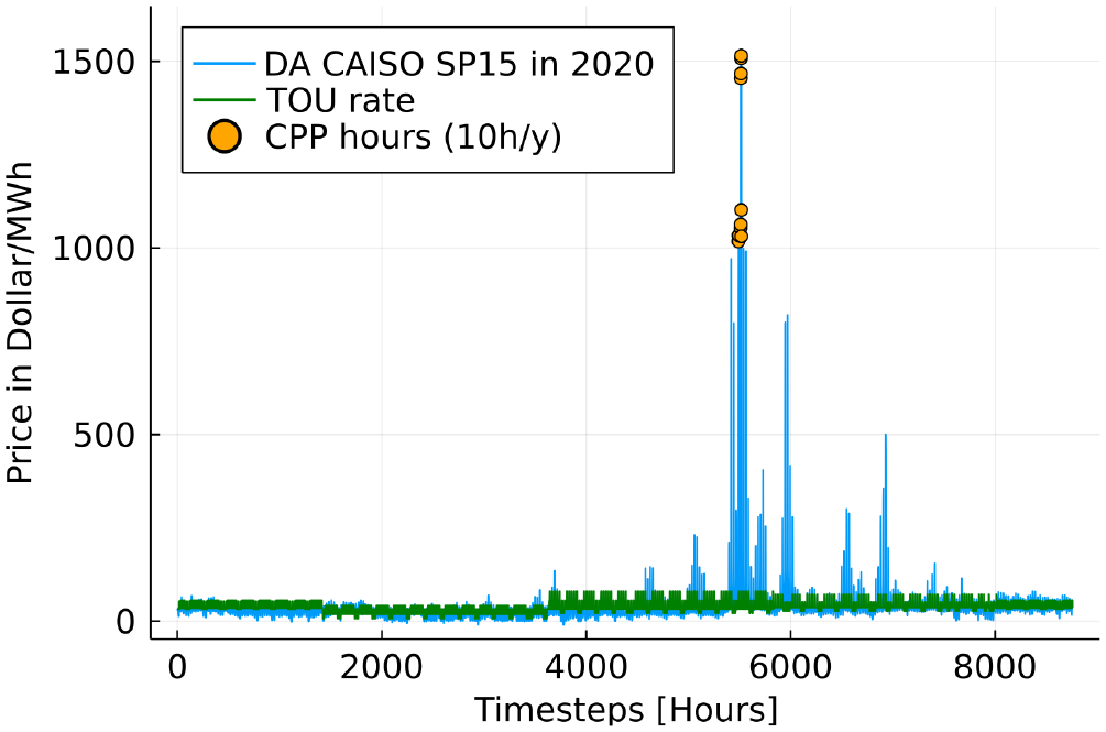
Day-ahead (DA) CAISO SP15 Hub prices in 2020, a calibrated TOU rate based on the preceding 3 years, and a CPP rate passing through the ten highest priced hours of the year.

For the example shown, the annual Pearson correlation is, respectively, 0.32 between spot prices and the TOU rate and 0.74 when adding the ten CPP hours to the TOU rate. Here, passing through the ten highest priced hours (0.1% of all hours, concentrated in two days) in the rate more than doubles the correlation.

Besides the annual Pearson correlation, we propose an alternative criterion to better reflect within-day load shifting incentives: the daily Spearman rank correlation. We use daily time series of hourly day-ahead prices as that is typically the time window during which shiftable appliances are scheduled. The rationale for considering rank correlations is that when scheduling an appliance, relative price differences at different times of day are more relevant than absolute price differences. The Spearman rank correlation measures how well TOU rates can capture relative within-day price differences and is less sensitive than the Pearson correlation to strong outliers-scarcity prices in the case of electricity markets. Figure 2 shows the spot price and TOU rate calibrated on historical prices for CAISO on January 6th of 2020 as an example.

Figure 2

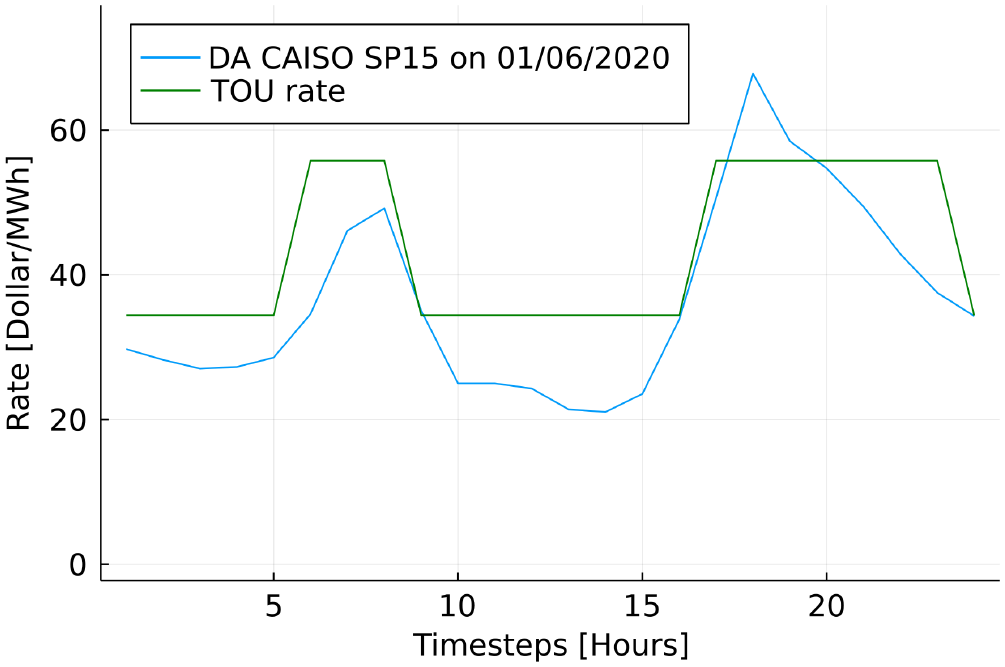
Day-ahead (DA) CAISO SP15 Hub prices for 01/06/’20 and a calibrated TOU rate based on the preceding 3 years (for details on the methodology to design the TOU rates, see Section 4)

We see that at least for that day, the TOU rate reasonably captures the relative price differences at different times of the day. Like the annual Pearson correlation, we also compute the daily Spearman correlations including the replacement of the TOU rate during the ten highest priced hours by the spot price in those hours. For the example shown in Figure 2, the daily Spearman correlation is 0.84. Adding CPP does not have an impact on the Spearman rank correlation for the day shown, as no high price event took place that day. The annual average of the daily Spearman correlations between the spot prices and the TOU rate with and without CPP for 2020 is 0.75.⁹ The impact of CPP is minimal because Spearman’s $ρ$ limits the impact of an outlier to the value of its rank.

The Spearman rank correlation is most directly relevant for loads that can be shifted easily within a day but not at all between days, while the Pearson correlation is most directly relevant for loads that can be reduced but not shifted. In fact, in addition to loads of these two polar types, some loads can only be shifted a few hours within days (cooking) with incurring disutility costs, and some can be shifted across days (clothes drying), again with disutility costs. The illustrative simulation model we now describe captures some of this diversity, but more research is clearly necessary to understand the quantitative importance of different varieties of load flexibility.

3.2 Simulation Models: Hourly Demand Functions and Load-shifting Optimization

In this section we first elaborate on the load-shifting optimization model and then we introduce the metric of interest that is computed based on the results of some illustrative simulations. In Appendix A, we briefly discuss the simulation approach based on hourly demand functions and provide a numerical example to explain the difference compared to the load scheduling optimization. We are critical of the simulation with hourly demand functions but use it to contrast the results of the load-shifting optimization. Different from Borenstein (2005), Holland and Mansur (2006), and Spees and Lave (2008), no equilibrium is calculated for either simulation model. The pricesensitive load is treated as a price taker. As long as the flexible load volumes are relatively small, this assumption is not expected to influence the results significantly. We come back to this simplification in the discussion (Section 6).

3.2.1 Formulation of the Load-shifting Optimization

The load-shifting optimization is inspired by the demand-flexibility module within the open-source capacity expansion model GenX (MIT Energy Initiative & Princeton University ZERO lab, 2022). Part of the total load is considered inflexible; the other part consists of several shiftable loads. In very simple terms, shiftable load is modelled as if that load is coupled with a battery that is constrained in how far in time it can move around load relative to a baseline consumption schedule (anticipate/delay) and that incurs a cost per MWh of displaced load. Below we explain in more detail the relevant equations. The parameterization of the load-shifting optimization model can be found in Appendix B. To be clear, this model has not been calibrated to real data, and our calculations should be viewed as illustrative.

The objective function (1) to be minimized is the cost of supplying the total load over T hours. T is the optimization horizon, which is 168 hours in our illustrative example.¹⁰ The first term represents the supply cost per hour with $p_{t}$ the time-varying retail rate and $L_{t}$ the final total load. The second term accounts for the cost of load shifting, with $Π_{t, f}$ the decrease in load of flexible load f in hour t relative to the baseline schedule and $v c_{f}$ the variable cost associated with shifting the flexible load f. This variable cost can be interpreted as the disutility cost of load shifting. For simplicity, the per kWh cost of shifting load does not depend on how far (within the load-specific constraints) the load is shifted, which is an important limitation as the size of the shift may affect costs in some real-world cases.

In our illustrative calculations there are $N = 10$ equal-sized flexible loads $(ρ_{f}^{\max} * δ_{f, t}) . ρ_{f}^{\max}$ is the maximum value of the flexible load over all time steps t, the sum of $ρ_{f}^{\max}$ over all flexible loads f adds up to 5 percent of total system load in our illustrative example. $δ_{f, t}$ determines the load shape. For example, imagine that flexible load f represents a fleet of EVs that have a total hourly charging capacity that adds up to $ρ_{f}^{\max}$ . In that case, the load will not be constant $(δ_{f, t} = 1$ ) but have a certain load shape over the course of the day. At any time t, the flexible demand that can be reduced or increased per hour relative to their baseline schedule $(ρ_{f}^{\max} * δ_{f, t})$ with a maximum time delay $(τ_{f}^{delay})$ and advancement $(τ_{f}^{advance})$ of the deferred or anticipated load, respectively.

\min . \sum_{t = 1}^{T} (p_{t} * L_{t} + \sum_{f = 1}^{N} v c_{f} * Π_{t, f})

(1)

s . t : L_{t} = \bar{L_{t, 0}} + \sum_{f = 1}^{N} Θ_{t, f} - \sum_{f = 1}^{N} Π_{t, f} \forall t

(2)

Γ_{t, f} = Γ_{t - 1, f} - Θ_{t, f} + Π_{t, f} \forall t \neq 1, f

(3)

Γ_{t, f} = Γ_{T, f} - Θ_{t, f} + Π_{t, f} t = 1, \forall f

(4)

Π_{t, f} \leq ρ_{f}^{\max} * δ_{f, t} \forall t, f

(5)

Θ_{t, f} \leq ρ_{t}^{\max} * δ_{f, t} \forall t, f

(6)

\sum_{e = t + 1}^{t + τ_{t + cty}^{tax}} Θ_{e, f} \geq Γ_{t, f} \forall t, f

(7)

\sum_{e = t + 1}^{t + τ_{f}^{astanee}} Π_{e, f} \geq - Γ_{t, f} \forall t, f

(8)

L_{t} \geq 0, Θ_{t, f} \geq 0, Π_{t, f} \geq 0, Γ_{t, f} free \forall t, f

(9)

Equation 2 describes the demand balance equation for the entire system in each hour t. The final load in any hour is equal the original load $(\bar{L_{t, 0}})$ , plus the sum of the changes in the $N$ flexible loads relative to their individual baseline schedules $(ρ_{f}^{\max} * δ_{f, t})$ . As above, $Π_{t, f}$ is the decrease in flexible load f in hour t relative to its baseline schedule, while $Θ_{t, f}$ is the increase in flexible load f in hour t relative to its baseline schedule.

Equations 3 -9 describe the constraints and variables of the flexible loads. Equations 3-4 keep track of the net loads shifted from each flexible load in each period $(Γ_{t, f}) \cdot$ ¹¹ Equations 5-6 ensure that the amount of demand that deviates from the baseline schedule does not exceed the maximum flexible demand that is available per hour. Equations 7-8 constrain the maximum hours of delay and anticipation of flexible loads, and (9) puts bounds on the variables.

3.2.2 The Relevant Metric: Realized Cost Reduction Potential [%]

We want to assess how well TOU(+CPP) rates replicate the incentives for load shifting that occur under dynamic pricing. In other words, we want to know whether TOU rates incentivize load to shift in the “right direction” (indicated by the observed hourly spot prices), especially when it matters most (i.e., during days when the differences between high and low hourly spot prices are the greatest). Therefore, we introduce a metric which we call the “realized cost reduction potential” (RCRP. The RCRP metric indicates how much of the reduction in average supply costs are obtained under an alternative time-varying rate (TOU or TOU+CPP) compared to the theoretical first best of load response to spot prices (Eq. 10). What we mean by the average supply cost under a certain rate design is the average spot price paid to serve the (partly) price-responsive load, after being exposed to an alternative time-varying rate. The more aligned the incentives provided by the alternative rate are with the spot price, the more beneficial load response under the alternative rate will be from a system point of view. In case the incentives for the load response under the alternative rate are perfectly aligned with the spot price, the average supply costs will be the same and the RCRP will be 100%. Note that RCRP can also be negative. This would be the case if TOU rates consistently incentivize load to shift from low to high observed spot prices.

RCRP = (FlatASC - AltASC) / (FlatASC - SpotASC)

(10)

With : FlatASC = \sum_{t = 1}^{T} (L_{t, 0} * {Spot}_{t}) / \sum_{t = 1}^{T} L_{t, 0}

(11)

\begin{matrix} SpotASC = \sum_{t = 1}^{T} (L_{t}^{Spot} * Spo t_{t} + β^{*} \sum_{f = 1}^{N} v c_{f} {* Π}_{t, f}^{Spot}) / \sum_{t = 1}^{T} L_{t}^{Spot} \end{matrix}

(12)

\begin{matrix} AltASC = \sum_{t = 1}^{T} (L_{t}^{TOU (+ CPP)} * Spo t_{t} + β^{*} \sum_{f = 1}^{N} v c_{f} {* Π}_{t, f}^{TOU (+ CPP)}) / \sum_{t = 1}^{T} L_{t}^{TOU (+ CPP)} \end{matrix}

(13)

To obtain the RCRP, we first calculate the average supply costs under the original inelastic load (FlatASC), which is equivalent to having a flat rate in place, as shown in Eq. 11. Next, we calculate the minimum average supply costs of the load (partially having a certain elasticity or a set of shiftable loads) under spot prices (SpotASC) as in Eq. 12, with $β$ being 0 in the case of the linear demand function and 1 in the case of the load-shifting optimization.¹² In the latter case, a variable cost for shifting load is accounted for. Importantly, the minimum average supply costs (SpotASC) assumes a constant optimization by consumers responding to daily updated hour-by-hour changes in spot prices, which is more complicated than standard TOU rates that vary depending on the time period within the day, day-type and season but are recurring and determined at least one year in advance. For that reason, the RCRP of a TOU rate might underestimate the performance of loadshifting responses under TOU relative to dynamic prices. Finally, in Eq. 13 the average supply cost under an alternative rate (TOU+(CPP)) is the load under the alternative rate multiplied by the spot price (AltASC).

4. TOU Rate Design Process

We compute four different TOU rate designs for the period 2014-2020 for each spot price series considered (CAISO SP15, ERCOT Houston Hub, and ISO-NE Boston Hub prices from 20112020). To limit complexity, and in line with observed practice, our TOU rates vary seasonally (four seasons), per day-type (two day-types) and within-day time blocks (depending on the TOU rate design). For all the TOU rate designs, the coefficients of the TOU rates, i.e., the magnitudes of the rates, are determined using regressions with the preceding three years of spot prices as dependent variables, i.e., a rolling 3 -year window of training data, with dummies per season (4), day-type (2) and the hours belonging to the different within-day TOU periods. Jacobsen et al. (2020) use the same regression approach to calibrate the TOU rates they study.¹³

The TOU coefficients are updated each year and scaled proportionally to make the loadweighted average price under any TOU rate equal to that under the observed hourly day-head spot prices.¹⁴ For the load data, we use hourly load data for 2014-2020 of the entire CAISO and ISO-NE system as no disaggregated load data for the specific hubs was available for the considered time period (S&P Global, 2022). For ERCOT, we used the more granular ERCOT Coast load data (ERCOT, 2022). The same load data are used in Section 5 in Figure 4 and for the computation of the results of the simulation models. Appendix C provides a complete overview explaining how the TOU rates are computed.

The TOU rate designs we use differ in how the hours in each day are divided into rate blocks:

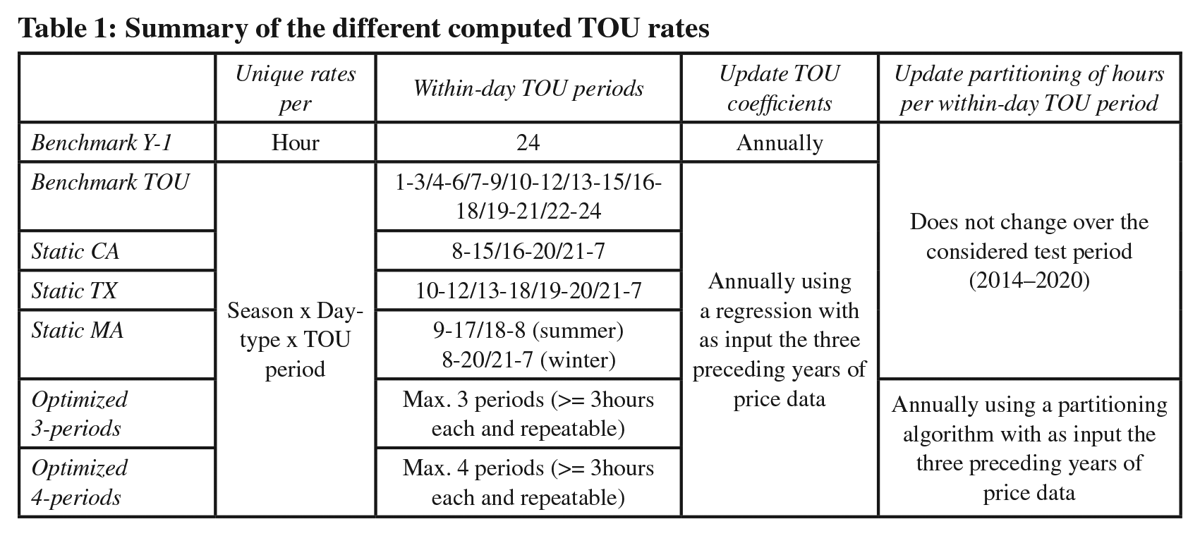
One benchmark TOU rate design with eight equally long within-day TOU periods of 3-hours each.

For each power system, one TOU rate design for which the partitioning of the different hours into TOU periods is inspired by existing TOU rates. The partitioning of the hours is kept constant over the years of the test period (2014-2020):

CA static: the TOU-D-4-9PM rate from Southern California Edison (SC&E, 2022) with three within-day periods: $8 am - 4 pm, 4 pm - 9 pm$ , and $9 pm - 8 am$ (only applied in weekdays and the same periods apply for all seasons)

TX static: an optional TOU rate plan in Texas (Shop Texas Electricity, 2021) with four within-day periods: $10 am - 1 pm, 1 pm - 7 pm, 7 pm - 9 pm$ , and 10pm-10am (only applied in weekdays and the same periods apply for all seasons)

MA static: a TOU rate offered for large commercial and industrial customers in the Boston area by Eversource (2022). There are two within-day periods during weekdays. In summer (June-September), there is a peak period from 9am-6pm and the remainder off-peak. For the rest of the year, the peak period is $8 am - 9 pm$ and the remaining hours are off-peak

Two TOU rate designs for which the partitioning of hours into TOU periods is calibrated based on the price patterns in the preceding three years and updated each year using a clustering algorithm based on Yang et al. (2019) and explained in Appendix C. We consider TOU designs with maximum three and maximum four periods within a day, labelled “Optimized 3-periods” and “Optimized 4-periods”.¹⁵ A period can be repeated within the same day (e.g., off-peak/shoulder/peak/shoulder with the same TOU rate in both shoulder periods for a day-type x season x year combination). We require from the algorithm that each within-day period needs to last at least three consecutive hours.

For the benchmark TOU design and the three TOU designs for which the period partitioning is based on existing TOU rates, we assume the within-day TOU periods to be the same for the four seasons and the two day-types. Also, we allow TOU coefficients to vary per within-day TOU time-block (thus not having a period being repeated within a day). This implies that for each year we obtain 64, 24, 32 and 16 unique TOU coefficients for the benchmark TOU, CA static, TX static, and MA static TOU designs, respectively.¹⁶ In that sense, these TOU designs that are inspired by existing TOU designs are slightly more advanced than those in practice. In practice, typically only two seasons (summer and the rest of the year) are considered, the different TOU periods are only introduced in weekdays, and it can be that periods are repeated within a day (e.g., off-peak during the night as well as around noon).¹⁷

Finally, we also introduce a benchmark Y-1 rate, which is the hourly day-ahead price of the preceding year during the same hour. This could be interpreted as the most extreme partitioning and implies 8760 rate coefficients. No data processing is needed for this benchmark.¹⁸ Table 1 provides a summary of the rate designs that we examine and the methods that we utilize.

Table 1

Summary of the different computed TOU rates

	Unique ratesper	Within-day TOU periods	Update TOUcoefficients	Update partitioning of hoursper within-day TOU period
Benchmark $Y - 1$	Hour	24	Annually	Does not change over the considered test period (2014-2020)
Benchmark TOU	Season x Day-type x TOU period	$1 - 3 / 4 - 6 / 7 - 9 / 10 - 12 / 13 - 15 / 16 -$ $18 / 19 - 21 / 22 - 24$	Annually using a regression with as input the three preceding years of price data
Static $CA$		$8 - 15 / 16 - 20 / 21 - 7$
Static $TX$		$10 - 12 / 13 - 18 / 19 - 20 / 21 - 7$
Static MA		9-17/18-8 (summer) 8-20/21-7 (winter)
Optimized 3-periods		Max. 3 periods $(> = 3$ hours each and repeatable)		Annually using a partitioning algorithm with as input the three preceding years of price data
Optimized 4-periods		Max. 4 periods $(> = 3$ hours each and repeatable)

5. Results

We first discuss the results of the time series analysis, then the results of the simulations.

5.1 Time Series Analysis: Annual Pearson Correlation and Daily Spearman Rank Correlation

Figure 3 shows the results for the out-of-sample annual Pearson correlation between the TOU rates without CPP (left panels) and with CPP (right panels) and the hourly day-ahead prices for the three power systems considered. We make two observations.

Figure 3

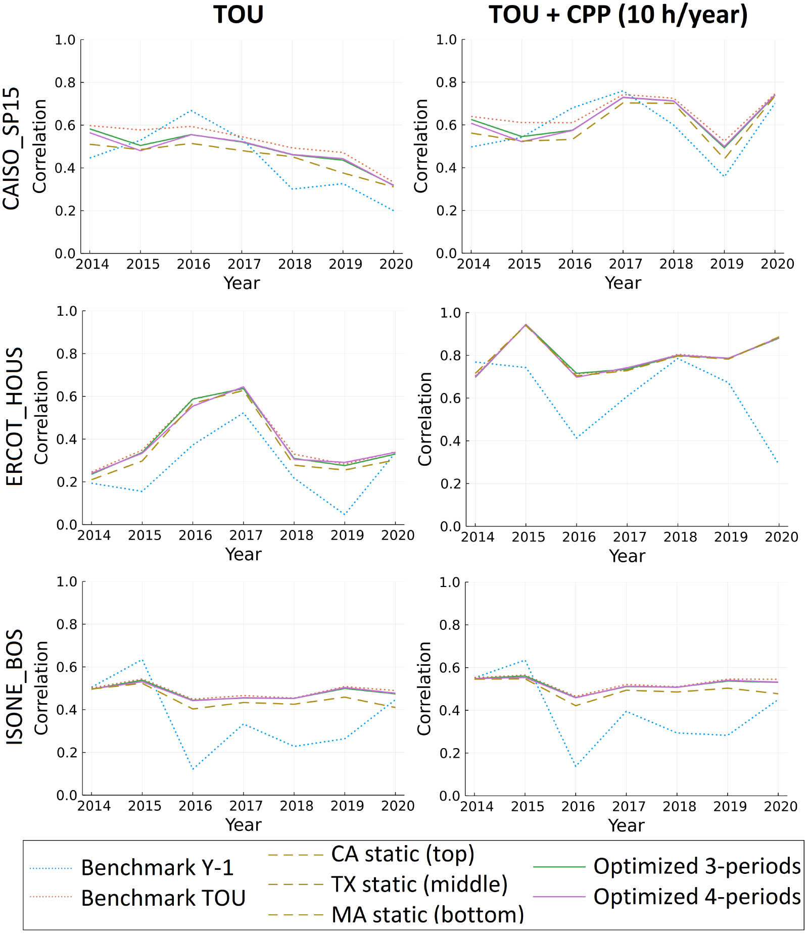
Annual Pearson correlations between the TOU rates without CPP (left panels) and with CPP (right panels) and the day-ahead prices for CAISO SP 15 (top), ERCOT Houston Hub (middle) and ISO-NE Boston Hub (bottom).

First, looking at the left panels, the Pearson correlations between TOU rates and the spot prices are rather low, in the range of $0.2 - 0.6$ . These results are in line with the existing literature (Hogan, 2014; Jacobsen et al., 2020), despite the large increase in the penetration of wind and solar in ERCOT and CAISO since 2014. We can see that the correlation depends on the power system, year, and, to a lesser extent, the TOU rate design.

Second, looking at the right panels, when replacing the TOU coefficients during the ten highest priced hours per year by the spot price during those hours, the out-of-sample Pearson correlation between TOU rates and the spot prices improves significantly for CAISO and, especially ERCOT, while the results for ISO-NE remain the same. Recall that ISO-NE is primarily a thermal system as of 2021. These results show that Pearson correlation results are to a very large extent driven by a few hours of very high prices, which are not captured by a TOU rate. This is confirmed when looking deeper at the day-ahead hourly price series of these power systems (shown in Appendix D); scarcity prices, both in frequency and magnitude, are most common in ERCOT, to a lesser extent in CAISO, and are mostly absent in ISO-NE.¹⁹ These results are a first indication of the usefulness of a CPP program targeting exactly these high price moments as a supplement to a stable TOU regime. The low correlations for Benchmark Y-1 are because it introduces very high prices during the wrong hours (the hours when very high prices occurred the year before).

Figure 4 shows the results for the out-of-sample average daily Spearman rank correlations between the TOU rates and the day-ahead prices (left panels). The results when complementing the TOU rates with CPP are almost identical to the ones shown and therefore not separately displayed. As stated before, in most cases scarcity price events happen during only a few days, thus only (mildly) impacting the daily rank correlations for those few days and not having an impact on the average over all the days of the year. Again, we make two observations.

Figure 4

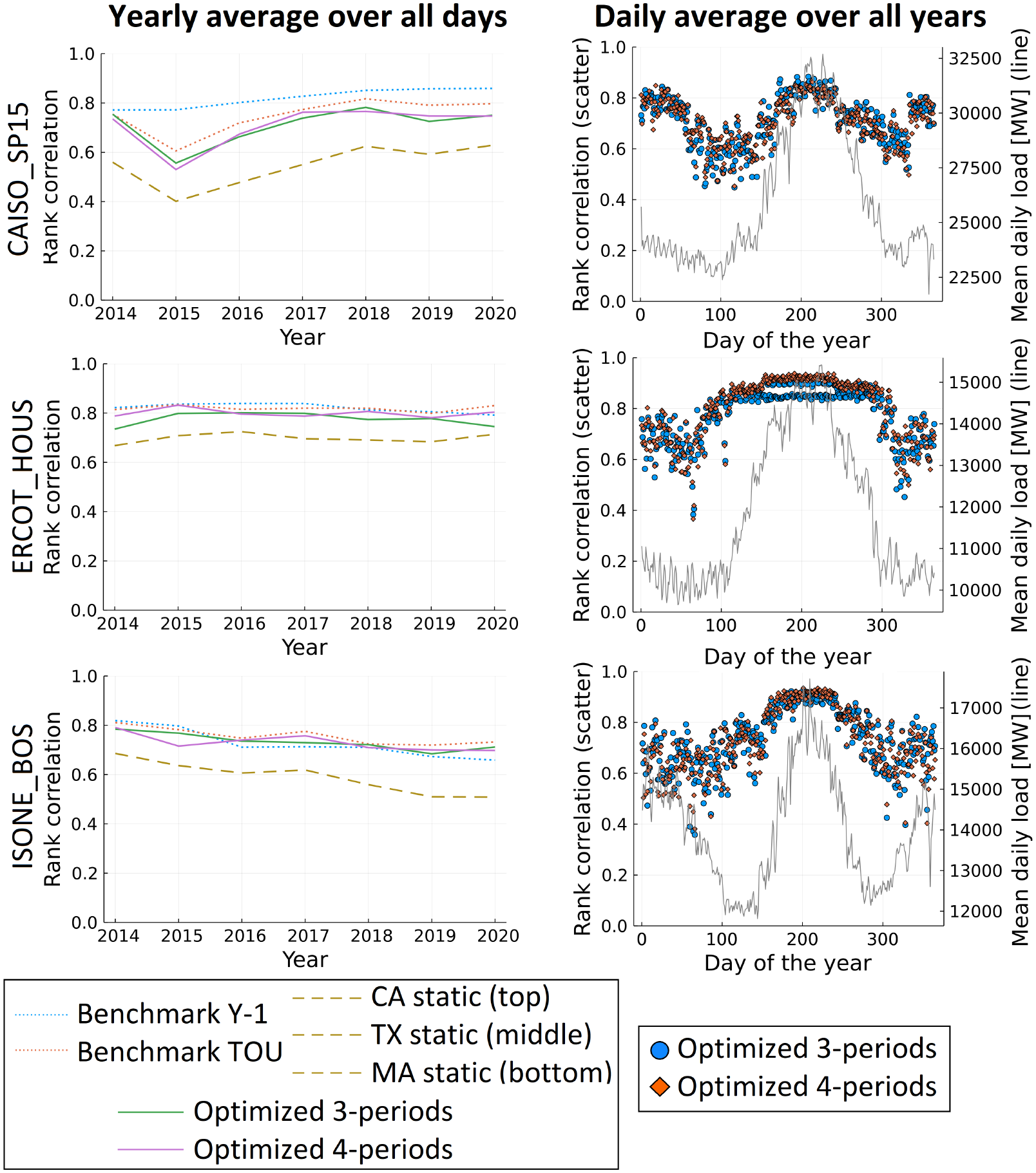
Yearly averaged daily Spearman rank correlations between the TOU rates and day-ahead prices (left panels) and the daily Spearman rank correlation between the TOU rates and spot prices when averaged per day in 2014-2020 (right panels) CAISO SP 15 (top), ERCOT Houston Hub (middle), and ISONE Boston Hub (bottom).

First, the average daily Spearman rank correlations are in almost all cases significantly higher than the annual Pearson correlations. The results illustrate that the computed TOU rates, while not able to capture sudden scarcity price events, are relatively good at anticipating the relative price differences within days. They give an indication that TOU rates can perform quite well in replicating the within-day load-shifting incentives provided by spot prices.

Second, the benchmark TOU rate design with many degrees of freedom and the TOU rate design with annually updated period partitioning ("Optimized 3/4-periods") perform significantly better than the static TOU designs with fewer, non-updated, within-day TOU periods. These results are explained by the fact that over time, as the supply and demand patterns change, with higher penetration of renewables with near-zero short-run marginal generating costs, the wholesale pricepatterns change.²⁰ Changes in price patterns require updating how within-day TOU periods are partitioned. If this is not done, as in the “static” TOU designs, the ability of TOU rates to anticipate relative within-day price differences is reduced. The alternative to regularly updating the partitioning of the hours in different within-day TOU periods is to allow for many within-day TOU periods, as in the benchmark TOU rate design. In that case, the TOU rate is very flexible and adjusts to changing price patterns merely by updating the (many) TOU coefficients on a yearly basis. But having many within-day TOU periods increases complexity. Having fewer TOU periods and gradually revising the exact partitioning of the hours belonging to the within-day TOU periods seems a more sensible approach.

In addition, we also show the daily Spearman rank correlation for each day of the year averaged over the seven years of the test period (2014-2020) for the two optimized TOU designs (right panels in Figure 4). On the $2^{nd} y$ -axis in the right panels in Figure 4 we show the load in the considered power system during that day of the year averaged over the same period. These figures show that the daily rank correlations have a strong seasonal pattern. The rank correlation is highest when the system load is highest. This indicates that when it matters most, the TOU rates are most likely to signal the correct relative price differences within each day.

5.2 Simulation Models: Hourly Demand Functions and Load-shifting Optimization

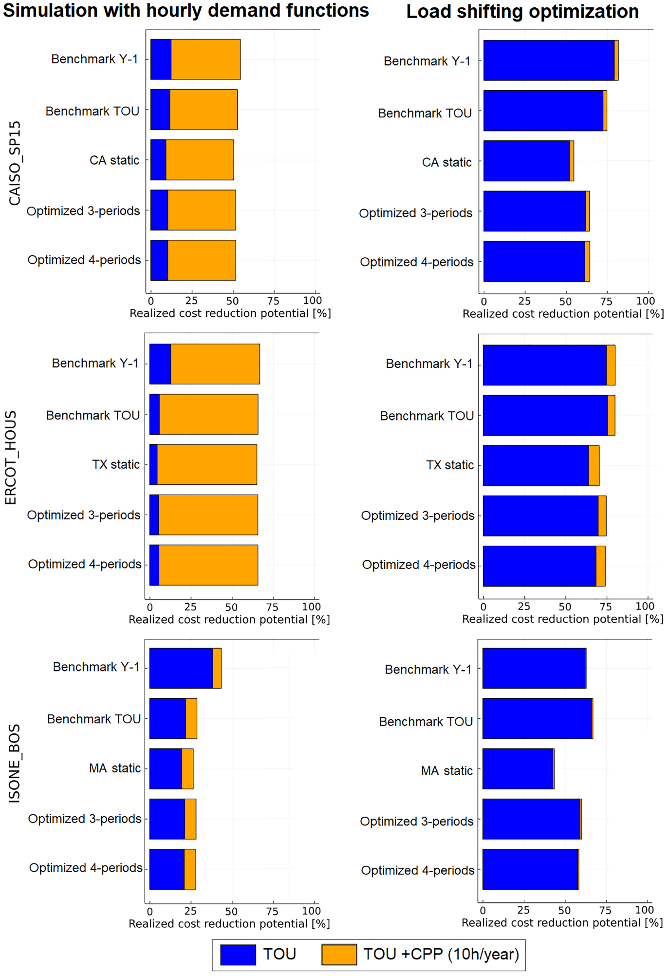
Figure 5 compares the results for the two simulation models for the different power systems. All results are relative to the first-best demand response under dynamic pricing considering a particular representation of demand, either hourly linear demand functions or, alternatively, a set of shiftable loads optimizing their schedule. For the hourly linear demand functions, we assume $50 %$ of (original) load to have a constant hourly elasticity of -0.1. The calibration of the loadshifting optimization can be found in Appendix B. We repeat that this model has not been calibrated to real data, and our calculations should be viewed as illustrative. We make three observations from Figure 5.

Figure 5

Left panels-Results for the realized cost reduction potential metric under linear hourly demand functions with a constant hourly elasticity of -0.1 for 50% of the load. Right panels-Results for the realized cost reduction potential metric under the load shifting optimization with 10 flexible loads with varying characteristics representing at maximum 5% of the peak load (Appendix B).

First, the results for both simulation models are very different. TOU rates perform significantly better under the load-shifting optimization model. An explanation is that under the hourly demand function (left panels), a significant share of the value of dynamic pricing lies in reducing demand during the few scarcity price hours. This is especially apparent from the results for ERCOT but also for CAISO. While TOU rates do not capture these scarcity price hours, CPP does, as illustrated for the same systems. This is less so the case for ISO-NE, as there are fewer scarcity events.

In the load-shifting optimization, the added value of CPP is significantly lower. The reason is that very high price events often happen during periods with already high prices (thus relatively high TOU rates). Contrary to the simulation with an hourly demand function, under the load-shifting optimization load is generally already scheduled away from these moments when such events are most likely to occur. This observation relates to Figure 4 (right panels), which shows that the relative price differences are easier to anticipate during the seasons in which load (and prices) are highest and scarcity events tend to occur, and thus demand flexibility is most valuable.²¹ This result reiterates the idea that for load shifting the relative price differences between hours matter a lot more than the absolute price differences between hours. On the other hand, as we discuss further below, in practice well-designed CPP regimes could likely induce sharper demand reductions than TOU rates by providing much stronger incentives or employing direct load control, in effect expanding the amount of flexible load. Thus Figure 5 likely understates the value of adding CPP to TOU pricing.

Second, the results for the ISO-NE power system, used as a sort of benchmark primarily thermal power system in this paper, are quite different from the results from CAISO and ERCOT, which are systems with significantly more intermittent renewables in the generation mix. This finding holds irrespectively of the way load response is characterized. The results for TOU rates under hourly demand functions for ISO-NE are in line with existing literature based primarily on thermal systems, i.e., TOU capturing about one fifth of the benefits of spot prices. Adding CPP to the TOU rates does not have a strong effect on the results for ISO-NE contrary to the other power systems. For the other power systems, the performance of TOU rates under hourly demand functions are even lower than in ISO-NE and are largely impacted by peak pricing events. Comparing the results of the load-shifting optimizations for all three power systems, better results are obtained for the systems with higher penetration of renewables, possibly due to more pronounced and relatively predictable multi-hourly price swings at times with very high or very low renewable output.

Third, when comparing the results for the TOU rate designs, in nearly all cases and independent of the representation of demand and the considered power system, the benchmark Y-1 performs best and the benchmark TOU second best. This means that prices lagged with one year are a relatively strong indicator of the relative price difference for the observed year, as also can be seen from the results for the rank correlations (Figure 4, left panels). The benchmark TOU gives many degrees of freedom and can also capture well the relative price differences. More importantly is that the more realistically implementable TOU designs with fewer periods (max. 3 or 4 per day) that are (slightly) revised from one year to another also perform relatively well (capturing $60 - 70 %$ of the theoretical maximum).

6. Discussion

This paper is a first attempt to analyze TOU(+CPP) rates in the context of easily shiftable within-day loads and power systems with increasing penetrations of intermittent renewables.

Considering the results from the time series analysis for CAISO SP15 and ERCOT Houston Hub, we confirm that the out-of-sample annual Pearson correlations between TOU rates and spot prices are low (averaging $0.3 - 0.5$ ) but show that these significantly improve when the spot price in a limited number of high-priced “scarcity” hours replaces the TOU rate in those hours (averaging 0.6-0.8). This reinforces the usefulness of CPP to deal with scarcity events (Blonz, 2022). These results are especially relevant for assessing the impacts of TOU/CPP rates on short-term load reductions. We find that out-of-sample daily Spearman rank correlations of TOU rates and spot prices are relatively high (averaging 0.7-0.8) and that rank correlations are especially high during summer when load is highest for all three systems (up to 0.9). This implies that, conditional upon power system characteristics and their specific design, TOU tariffs can provide a high proportion of socially efficient load-shifting incentives. Further, the simulation models confirm the intuition that the relative performance of TOU rates, complemented or not with a CPP program, compared to dynamic pricing is largely determined by how flexible load is characterized, i.e., responding to hour-to-hour differences in price levels or shifting load from high to low price periods (typically within a day).

Based on these results and considering that demand flexibility, especially at the residential and small commercial level, is expected to increasingly manifest itself in different forms of load shifting, we can say that TOU rates can better replicate incentives that would result from spot prices signals than previously assumed in the literature. This holds especially true for CAISO SP15 and ERCOT Houston Hub, systems with relatively high penetrations of wind and solar. The results for ISO-NE, acting as a control representing the thermal-dominated systems upon which many of the previous papers relied, indicate that these findings are to a certain extent conditional upon changesin the supply mix but that the introduced alternative assessment criteria play a bigger role. Overall, TOU rates, when having yearly updated coefficients and within-day periods based on historical data, perform well in indicating relative price differences within days, and, as such, provide relatively effective load-shifting incentives.

While TOU rates do not capture sudden scarcity price events, it is important to note that important peak pricing events often occur within periods of relatively high prices. As such, flexible load, reacting to relative price differences, already has an incentive to reduce load during those scarcity price events just by having TOU rates in place. In practice, of course, there is significant value in mobilizing additional demand reduction during those moments via well-designed CPP programs. In that regard, complementing TOU rates with a CPP program is valuable. The value of CPP can be seen to a certain extent in the results shown in Figure 5 (right panels) but would be even more pronounced if additional “emergency demand shifting/reduction potential” were added to the modelling. Methodologically, this is not complicated; the question is what the ratio is between “regular flexible intraday shiftable load” (e.g., charging an EV) versus “emergency demand shifting/reduction potential” (e.g., rather abruptly stopping an air conditioner for two hours when it is hot and accepting less comfort for a monetary reward). This ratio will depend on the power system and the CPP program.

With regards to the implementation of a CPP program, we recommend promoting load control programs where, e.g., at the reward of a discount on the bill, a third party (LSE or other) can regulate an appliance for a limited period. We prefer such an approach over actually passing through very high prices during scarcity price moments. The former approach is also how we model the CPP program: as if a third-party entity sees the very high spot price and schedules the load accordingly. The latter approach of passing through the very high spot prices is not in line with one of the main reasons for considering alternative rate designs, namely keeping the electricity bill predictable. Significantly increased rates to a level between the regular TOU rate and the actual spot price during scarcity events might be an approach in the middle. However, we tend to think that load control with an option to opt out (e.g., overriding load control and giving up the price discount) will perform better than having consumers react to an unexpected increased rate during scarcity events.

Two methodological limitations of the current analysis and two future sensitivity analyses seem particularly important.

Regarding the methodological aspects, first, a limitation of our simulation models is that we modelled flexible load as a price taker. With increasing load flexibility, shifts in demand will in turn impact wholesale spot prices. A more holistic welfare analysis would be required to capture this effect. Second, we did not include cross-elasticities in the simulation approach with hourly demand functions. Doing so could, to a certain extent, replicate load shifting. However, calibrating the cross-elasticities to replicate the outcome as under the load-shifting optimization is far from a trivial problem.

Regarding the sensitivity analysis, first, we considered several alternative TOU rate designs, but more analysis can be done regarding the simplicity versus efficiency trade-off for TOU rate designs. We need to investigate in more depth which parameters have the most significant impact on the performance of TOU rates relative to dynamic pricing. Second, and most important, it is unclear whether our findings will still hold in future heavily decarbonized power systems dominated by solar PV, wind, and different types of storage. It might be that the relative price differences within a day are a lot harder to anticipate than at present. In such a context, other, more complicated, retail rate plans may need to be developed. Examples of such ideas are having consumers hedge part of their load while real-time deviations from the contracted capacity are settled at spot prices (Chao, 2011; Wolak and Hardman, 2020) or the introduction of an insurance mechanism that accompanies the passed-through spot prices to consumers $\neg$ see e.g., Batlle et al. (2022a, 2022b). The cost of the insurance could be a function of the extent to which load control is granted by the consumer to the insurance provider. The more complex the rate design, however, the less certain one can be about the responses by small customers.

7. Conclusion and Policy Recommendations

Increasing volatility in wholesale prices due to high penetrations of intermittent renewables with near-zero short-run marginal generating costs on the supply side and expanding opportunities to shift loads on the demand side increases the efficiency gains that can be made by the introduction of time-varying retail rates. The theoretical first-best solution of passing through wholesale spot energy prices to consumers is not widely popular now, as consumers typically place a high value on predictability and bill stability, and we expect it to be even less popular in the future as spot prices become more volatile. We have introduced novel criteria to assess how well second-best alternatives, time-of-use (TOU) and critical peak pricing (CPP), can replicate the incentives to shift load that are provided via spot price signals. The proposed assessment criteria are tailored to a context with increasingly shiftable load, such as the charging of electric vehicles and cycling heat pumps. We have computed results using historical data from three diverse power systems: CAISO, ERCOT, and ISO-NE.

We conclude that well-designed TOU rates, especially when accompanied with a CPP program involving load control during infrequent scarcity price events, are more attractive from an efficiency perspective than the existing literature suggests. We recommend the acceleration of the adoption of TOU rates (e.g., rather than being opt-in, making TOU rates the default with the possibility to opt-out) accompanied by CPP as a valuable intermediate step towards improved retail electricity rates that balance efficiency considerations and consumer/political pressures for price predictability and bill stability. An important question, which we plan to investigate, is whether the results presented here still hold in systems with significantly higher penetration of intermittent renewables and storage. In any case, we urge more research to investigate retail rate plans potentially including hedging and/or insurance mechanisms.

Supplemental Material

sj-pdf-1-enj-10.5547_01956574.45.3.tsch – Supplemental material for Electricity Retail Rate Design in a Decarbonizing Economy: An Analysis of Time-of-use and Critical Peak Pricing

Supplemental material, sj-pdf-1-enj-10.5547_01956574.45.3.tsch for Electricity Retail Rate Design in a Decarbonizing Economy: An Analysis of Time-of-use and Critical Peak Pricing by Tim Schittekatte, Dharik Mallapragada, Paul L. Joskow and Richard Schmalensee in The Energy Journal

Footnotes

Appendix A: The Hourly Demand Function Simulations and a Numerical Example

Borenstein (2005), Holland and Mansur (2006), and Spees and Lave (2008) represent flexibility in the consumption of electricity via hourly linear demand functions. The discretized version of a linear demand function is provided by Eq. A.1. With $L_{t}$ being the total load afterexposure to a time-varying rate in hour $t, α_{t}$ being the fraction of the load that is considered flexible in hour $t, \bar{L_{t, 0}}$ being the total original (anchor) load in hour $t, ε_{t}$ the elasticity which can vary from one hour to another, $P_{t}$ the retail rate for the hour $t$ , and $\bar{P_{0}}$ the original flat rate for the year.

(A.1)

\begin{matrix} L_{t} = \bar{L_{t, 0}} + ε_{t} * \frac{α_{t} * \bar{L_{t, 0}}}{\bar{P_{0}}} * (P_{t} - \bar{P_{0}}) \end{matrix}

The original flat rate for the year is calculated as the load-weighted average price of the spot prices.²² In simple terms, the elastic portion of the load increases when prices are lower than the flat rate and vice-versa, and the magnitude of change is proportional to the difference between the flat rate and the time-varying rate.

The left panels in Figure A.1 show an example of the impact of, respectively, spot prices (top) and a TOU rate (bottom) on the aggregated load profile of CAISO of 01/06/’22 under the assumption of an hourly linear demand function. We assume $50 %$ of (original) load to have a constant hourly elasticity of -0.1. At least for the considered day, the load response is not very different under both rates. The right panels in Figure A.1 show an example of the impact of, respectively, spot prices (left) and a TOU rate (right) on the aggregated load profile of CAISO of 01/06/’22 under the assumption of a load-shifting optimization. Ten flexible loads with varying characteristics are modelled, in total representing at maximum $5 %$ of the maximum system load. The parameters are described in Appendix B.2.

When comparing the left and right panels of Figure A.1, we can note for example that the load response in the morning peak (7-10am) is higher for the load optimization relative to the linear demand function, especially under dynamic pricing. This is an illustration of the major difference between these approaches. The hourly demand function responds to absolute price differences compared to an anchor price (which is limited for the morning peak), while the load-shifting optimization is sensitive to relative price differences within the day (which are significant for the morning peak versus the adjacent hours in the night and around noon). Another manifestation of the difference between both approaches of modelling demand can be seen in the hours 10-12 and 14-17 under the TOU tariffs. For the simulation with hourly demand functions, there is nearly no change in the load compared to the baseline as the TOU price is very close to the anchor price. In contrast, for the load-shifting optimization, the load increases during those moments as, respectively, some load that was deferred during the morning peak is satisfied “in delay” and some load is satisfied “in advance” to allow for a load reduction during the evening peak.

Appendix B: Parameters for the Numerical Example of the Loadshifting Optimization

Table B.1 summarizes the key parameters used for the numerical example of the loadshifting optimization. This parameterization does not intend to replicate the characteristic of a specific real-world flexible load but serves an illustrative purpose. Each flexible load has the maximum size $(ρ_{f}^{\max})$ but a different load shape $(δ_{f, t})$ . The maximum total flexible load $(ρ_{f}^{\max})$ across all hours is $5 %$ of the highest demand in the specific power system observed during the test period (2014-2020). $δ_{f, t}$ is randomized in this illustrative example due to a lack of representative data. Further sensitivity analysis with a characterization of loads inspired by certain real-world loads is a possibility for future work. For example, $δ_{f, c}$ could in the future be calibrated to reflect temporal variations in, for example, the amount of EVs plugged-in or the heating load for a group of well-insulated houses. There might be a minor impact of the characterization of the flexible load on the exact results of the load-shifting optimization shown in Figure 5, but no qualitative differences are expected, as all results are computed relative to the load-shifting response under dynamic pricing for the same flexible loads. Please note that we include two flexible loads with very high variable cost for shifting, respectively 75 and $150 $ / MWh$ , for which there is a lot of flexibility in their scheduling. These loads are thought as being “emergency load-shifting options” and are only active under scarcity price events (via spot prices or CPP event).

Appendix C: Details on the TOU Rate Design Process

This appendix is split into two parts. First, we discuss the different steps of the TOU rate design process. Afterward, we provide more detailed information about the TOU partitioning algorithm.

Appendix D: Day-Ahead Price Series for the Power Systems

Please note that the y-axis has a different scale for each time series.

Appendix E: Illustrations of Changing Price Patterns from 2011-2020

Figure E.1 -3 show the average normalized price profiles for working days per season per considered power system for the period of 2011-2020. These figures give an intuition that the optimal within-day partitioning of hours into TOU periods evolves over the years. This particularly the case for the CAISO SP15 data.

The raw day-ahead price data is processed in four steps. First, the days are sorted per year, season, and day-type. Second, each day is normalized by dividing all prices per day by the maximum price of that day. Third, the average of the normalized prices for a particular hour in a particular year, season and day-type is calculated. Fourth, the average normalized price profile is plotted per year, season, and day-type. We work with prices that are normalized to avoid scarcity prices having an excessive impact on the “typical” price profiles per year, season, and day-type.

Acknowledgements

The authors want to acknowledge the MIT Energy Initiative’s Future Energy Systems Center for research support. We also thank our colleagues Carlos Batlle, John Parsons, Robert Stoner, Theodore Black, Michael Giovanniello, and Graham Turk for valuable discussions. Further, we thank participants of the FERC Technical Conference on Increasing Market and Planning Efficiency (June 2022), the $43^{rd}$ IAEE International Conference (July 2022), and the CEEPR & EPRG International European Energy Policy Conference (September 2022) for valuable feedback.

Notes

References

Batlle

Carlos

Schittekatte

Tim

Knittel

Christopher R.

(2022a). “Power Price Crisis in the EU: Unveiling Current Policy Responses and Proposing a Balanced Regulatory Remedy.” CEEPR WP 2022-004. https://doi.org/10.2139/ssrn.4044848.

Batlle

Carlos

Schittekatte

Tim

Knittel

Christopher R.

(2022b). “Power Price Crisis in the EU 2.0+: Desperate Times Call for Desperate Measures.”MITEI WP-2022-02. https://doi.org/10.2139/ssrn.4074014.

Blonz

Joshua A.

(2022). “Making the Best of the Second-Best: Welfare Consequences of Time-Varying Electricity Prices.”Journal of the Association of Environmental and Resource Economists Forthcoming. https://doi.org/10.1086/720566.

BNEF (2022). “Electric Vehicle Outlook 2022.”https://about.bnef.com/electric-vehicle-outlook/.

Boiteux

Marcel

(1949). “La Tarification Des Demandes En Pointe: Application de La Theorie de La Vente Au Cout Marginal.”Revue Générale de l’électricité 58:321-40.

Borenstein

Severin

(2005). “The Long-Run Efficiency of Real-Time Electricity Pricing.”The Energy Journal 26(3): 93-116. https://doi.org/10.5547/ISSN0195-6574-EJ-Vol26-No3-5.

Borenstein

Severin

Holland

Stephen

(2005). “On the Efficiency of Competitive Electricity Markets with Time-Invariant Retail Prices.”The RAND Journal of Economics 36(3): 469-93.

Borlaug

Brennan

Salisbury

Shawn

Gerdes

Mindy

Muratori

Matteo

(2020). “Levelized Cost of Charging Electric Vehicles in the United States.”Joule 4(7): 1470-85. https://doi.org/10.1016/j.joule.2020.05.013.

Busby

Joshua W.

Baker

Kyri

Bazilian

Morgan D.

Gilbert

Alex Q.

Grubert

Emily

Rai

Varun

Rhodes

Joshua D.

Shidore

Sarang

Smith

Caitlin A.

Michael E.

Webber

(2021). “Cascading Risks: Understanding the 2021 Winter Blackout in Texas.”Energy Research and Social Science 77: 102106. https://doi.org/10.1016/j.erss.2021.102106.

10.

California Energy Commission (2022). “California Electricity Data.”https://www.energy.ca.gov/data-reports/energyalmanac/california-electricity-data.

11.

Chao

Hung-po

(2011). “Demand Response in Wholesale Electricity Markets: The Choice of Customer Baseline.”Journal of Regulatory Economics 39(1): 68-88. https://doi.org/10.1007/s11149-010-9135-y.

12.

CPUC (2022). “Advanced Strategies for Demand Flexibility Management and DER Customer Compensation.”Energy Division White Paper and Staff Proposal.

13.

EIA (2022). “FAQ: How Many Smart Meters Are Installed in the United States, and Who Has Them?”https://www.eia.gov/tools/faqs/faq.php?id=108&t=3

14.

Ekholm

Tommi

Virasjoki

Vilma

(2020). “Pricing and Competition with 100% Variable Renewable Energy and Storage.”The Energy Journal 41: 215-31. https://doi.org/10.5547/01956574.42.S12.tekh.

15.

ERCOT (2021). “ERCOT State of the Grid 2020.”https://www.ercot.com/files/docs/2021/06/07/ERCOTSOG2020_Final.pdf.

16.

ERCOT (2022). “Hourly Load Data Archives.”2022. https://www.ercot.com/gridinfo/load/load_hist.

17.

Eversource (2022). “2022 Summary of Eastern Massachusetts Electric Rates of the Greater Boston Service Area.”2022. https://www.eversource.com/content/docs/default-source/rates-tariffs/ema-greater-boston-rates.pdf?sfvrsn=c27ef362_40.

18.

Faruqui

Ahmad

Sergici

Sanem

(2013). “Arcturus : International Evidence on Dynamic Pricing.”The Electricity Journal 26(7): 55-65. https://doi.org/10.1016/j.Tej.2013.07.007.

19.

Faruqui

Ahmad

Sergici

Sanem

Lam

Long

(2020). “Bridging the Chasm between Pilots and Full-Scale Deployment of Time-of-Use Rates.”The Electricity Journal 33(10): 106857. https://doi.org/10.1016/j.tej.2020.106857.

20.

Hausman

William J.

Neufeld

John L.

(1984). “Time-of-Day Pricing in the U.S. Electric Power Industry at the Turn of the Century.”The RAND Journal of Economics 15(1): 116-26. https://doi.org/10.2307/3003674.

21.

Herter

Karen

(2007). “Residential Implementation of Critical-Peak Pricing of Electricity.”Energy Policy 35: 2121-30. https://doi.org/10.1016/j.Enpol.2006.06.019.

22.

Hogan

William W.

(2014). “Time-of-Use Rates and Real-Time Prices.”1-8. http://www.hks.harvard.edu/fs/whogan/Hogan_TOU_RTP_Newark_082314.pdf.

23.

Holland

Stephen P.

Mansur

Erin T.

(2006). “The Short-Run Effects of Time-Varying Prices in Competitive Electricity Markets.”The Energy Journal 27(4): 127-55. https://doi.org/10.5547/ISSN0195-6574-EJ-Vol27-No4-6.

24.

IEA (2021). “Heat Pumps.”https://www.iea.org/reports/heat-pumps.

25.

ISO-NE (2022a). “Resource Mix.”2022. https://www.iso-ne.com/about/key-stats/resource-mix.

26.

ISO-NE (2022b). “Solar Power in New England: Concentration and Impact.”https://www.iso-ne.com/about/what-we-do/indepth/solar-power-in-new-england-locations-and-impact.

27.

Jacobsen

Mark R.

Knittel

Christopher R.

Sallee

James M.

Van Benthem

Arthur A.

(2020). “The Use of Regression Statistics to Analyze Imperfect Pricing Policies.”Journal of Political Economy 128(5): 1826-76. https://doi.org/10.1086/705553.

28.

Joskow

Paul L.

(1976). “Contributions To the Theory of Marginal Cost Pricing.”The Bell Journal of Economics 7(1): 197206. https://doi.org/10.2307/3003196.

29.

Joskow

Paul L.

Wolfram

Catherine D.

(2012). “Dynamic Pricing of Electricity.”American Economic Review 102(3): 381-85. https://doi.org/10.1257/aer.102.3.381.

30.

Kavulla

Travis

(2023). “Why Is the Smart Grid So Dumb? Missing Incentives in Regulatory Policy for an Active Demand Side in the Electricity Sector.”White Paper from the Energy Systems Integration Group. https://www.esig.energy/aligningretail-pricing-with-grid-needs.

31.

Liang

Jing

Liu

Pengfei

Qiu

Yueming

Wang

Yi David

Xing

(2020). “Time-of-Use Electricity Pricing and Residential Low-Carbon Energy Technology Adoption.”The Energy Journal 41(3). https://doi.org/10.5547/01956574.41.2.jlia.

32.

Littlechild

Stephen

Kiesling

Lynne

(2021). “Hayek and the Texas Blackout.”The Electricity Journal 34(6): 106969. https://doi.org/10.1016/j.tej.2021.106969.

33.

Mallapragada

Dharik S.

Junge

Christian

Wang

Cathy

Pfeifenberger

Hannes

Joskow

Paul L.

Schmalensee

Dick

(2021). “Electricity Pricing Problems in Future Renewables-Dominant Power Systems.” CEEPR WP 2021-017-R. November 2021 (Revised February 2022). https://doi.org/10.2139/ssrn.4037741.

34.

Mays

Jacob

Klabjan

Diego

(2017). “Optimization of Time-Varying Electricity Rates.”The Energy Journal 38(5): 67-91. https://doi.org/10.5547/01956574.38.5.jmay.

35.

MIT Energy Initiative, and Princeton University ZERO lab (2022). “GenX: A Configurable Power System Capacity Expansion Model for Studying Low-Carbon Energy Futures.”https://github.com/GenXProject/GenX.

36.

PG&E (2022). “Find out If Peak Day Pricing Is Right for Your Business.”https://www.pge.com/en_US/small-mediumbusiness/your-account/rates-and-rate-options/peak-day-pricing.page.

37.

Qiu

Yueming

Colson

Gregory

Wetzstein

Michael E.

(2017). “Risk Preference and Adverse Selection for Participation in Time-of-Use Electricity Pricing Programs.”Resource and Energy Economics 47: 126-42. https://doi.org/10.1016/jreseneeco.2016.12.003.

38.

S&P Global (2022). “Energy Dataset.”https://www.spglobal.com/en/.

39.

SC&E (2022). “TOU Rate Plans.”https://www.sce.com/residential/rates/Time-Of-Use-Residential-Rate-Plans.

40.

Schittekatte

Tim

Mallapragada

Dharik S.

Joskow

Paul L.

Schmalensee

Richard

(2023). “Reforming Retail Electricity Rates to Facilitate Economy-Wide Decarbonization.”Joule Forthcoming. https://doi.org/10.1016/j.joule.2023.03.012.

41.

Schweppe

Fred C.

Caramanis

Michael C.

Tabors

Richard D.

Bohn

Roger E.

(1988). Spot Pricing of Electricity. Kluwer Academic Publishers.

42.

Shop Texas Electricity (2021). “Off-Peak Electricity Rates: Are Your Electricity Rates Cheaper at Night?”https://blogshoptexaselectricity.com/off-peak-electricity-rates-are-your-electricity-rates-cheaper-at-night/.

43.

Spees

Kathleen

Lave

Lester

. 2008. “Impacts of Responsive Load in PJM : Load Shifting and Real-Time Pricing.”The Energy Journal 29 (2): 101-21. https://doi.org/10.5547/ISSN0195-6574-EJ-Vo129-No2-6.

44.

Spees

Kathleen

Newell

Samuel A.

Pfeifenberger

Johannes P.

(2013). “Capacity Markets-Lessons Learned from the First Decade.”Economics of Energy & Environmental Policy 2(2): 1-26. https://doi.org/10.5547/2160-5890.2.2.1.

45.

Steiner

Peter O.

(1957). “Peak Loads and Efficient Pricing.”The Quarterly Journal of Economics 71(4): 585-610. https://doi.org/10.2307/1885712.

46.

Trabish

H.K.

(2022). “Outlook: A New Recognition Is Coming of Rate Design’s Critical Role in the Energy Transition.” Published on Jan. 19, 2022, in Utility Dive. 2022. https://www.utilitydive.com/news/2022-outlook-a-new-recognition-iscoming-of-rate-designs-critical-role-in/611756/.

47.

Turvey

Ralph

(1968). Optimal Pricing and Investment in Electricity Supply. Cambridge: M.I.T. Pres.

48.

Vijay

Avinash

Fouquet

Nicolas

Staffell

Iain

Hawkes

Adam

(2017). “The Value of Electricity and Reserve Services in Low Carbon Electricity Systems.”Applied Energy 201: 111-23. https://doi.org/10.1016/j.Apenergy.2017.05.094.

49.

Wolak

Frank A.

Hardman

I.H.

(2020). “The Future of Electricity Retailing and How We Get There.”Lecture Notes in Energy 41. https://doi.org/10.1007/978-3-030-85005-0_7.

50.

Wolak

Frank A.

(2011). “Do Residential Customers Respond to Hourly Prices? Evidence from a Dynamic Pricing Experiment.”American Economic Review: Papers & Proceedings 101: 83-87. https://doi.org/10.1257/aer.101.3.83.

51.

Xcel Energy (2022). “Load Management Pilot Standard Offer Program.”https://tx.my.xcelenergy.com/s/business/rate-plans/load-management-pilot.

52.

Yang

Hejun

Wang

Lei

Zhang

Yeyu

Tai

Heng Ming

Yinghao

Zhou

Ming

(2019). “Reliability Evaluation of Power System Considering Time of Use Electricity Pricing.”IEEE Transactions on Power Systems 34(3): 1991-2002. https://doi.org/10.1109/TPWRS.2018.2879953.

53.

Zhou

Ella

Hale

Elaine

Present

Elaina

(2022). “Building Flexibility Revenue in Modeled Future Bulk Power Systems with Varying Levels of Renewable Energy.”Heliyon 8(7): e09865. https://doi.org/10.1016/j.heliyon.2022.e09865.

Supplementary Material

Please find the following supplemental material available below.

For Open Access articles published under a Creative Commons License, all supplemental material carries the same license as the article it is associated with.

For non-Open Access articles published, all supplemental material carries a non-exclusive license, and permission requests for re-use of supplemental material or any part of supplemental material shall be sent directly to the copyright owner as specified in the copyright notice associated with the article.

0.00 MB

0.07 MB