Sage Journals: Discover world-class research

Abstract

Evidence of an association between survival time and date of birth would suggest an etiologic role for a seasonally variable environmental exposure occurring within a narrow perinatal time period. Risk factors that may exhibit seasonal epidemicity include diet, infectious agents, allergens, and antihistamine use. Typically data has been analyzed by simply categorizing births into months or seasons of the year and performing multiple pairwise comparisons. This paper presents a statistically robust alternative, based upon a trigonometric Cox regression model, to analyze the cyclic nature of birth dates related to patient survival. Disease birth-date results are presented using a sinusoidal plot with peak date(s) of relative risk and a single P value that indicates whether an overall statistically significant seasonal association is present. Advantages of this derivative-free method include ease of use, increased power to detect statistically significant associations, and the ability to avoid arbitrary, subjective demarcation of seasons.

Keywords

sinusoidal Cox regression seasonality of birth

Introduction

The fetal origin hypothesis purports that early life environmental exposures may influence disease phenotype in adulthood.¹ Accordingly, individuals born during a specific season may experience unique exposures at a time when they are particularly sensitive to such exposures. A key premise of the theory is that certain exposures and experiences around the time of birth lead to adaptive phenotypes that better prepare the individual for events that may occur later in life. However, not all developmental adaptations have an apparent value in modern society, such as the disruptive response to a host of man-made teratogens.

Experts have hypothesized an etiologic link between season of birth and various childhood diseases, in particular cancer.^2–5 This is partly due to the temporal brevity between the perinatal window of susceptibility to environmental carcinogens and disease development. This narrow age-dependent period is characterized by rapid cell growth and division and an undeveloped immune system..^6,7 Various chemicals and oncogenic viruses have been shown in the laboratory to induce developmental cancers when specifically administered during perinatal life versus maturity.^{8 –10} Infectious agents, pesticides, anti-histamines, indoor environmental tobacco smoke, and vitamin D are a few environmental exposures that tend to follow a seasonal pattern and conceivably may play a role in disease risk or protection.¹¹

There also is evidence suggesting that prenatal and early childhood exposures may play a role in adult diseases. For example, exposure to airborne infections during infancy has been associated with increased mortality from similar infections in old age.¹² A birth cohort from 1634 through 1870 in the small village on Minorca Island, Spain was used to demonstrate decreased mortality among summer births, thus suggesting the importance of early seasonal exposures in disease development decades later.¹ Similarly, seasonal birth exposures have been implicated in some adult cancers.¹¹

Evidence of an association between season of birth and childhood disease would suggest that a seasonally variable environmental exposure may underlie the disease. The type, nature, timing, and severity of the exposure ultimately may be important determinants of whether a seasonal factor has long-term negative or positive consequences for disease development and patient survival.

To the best of our knowledge, no studies have examined day of birth as a seasonal determinant of survival time, when controlling for outcome related covariates. This paper presents a simple method to determine the statistical significance of a seasonal risk factor in a Cox regression model that allows for control of confounding variables.

Methodology

Cox regression, also known as the proportional hazards model, is a continuous time technique in which event rates vary instantaneously as a function of time.^13–15 A common use of Cox regression is to estimate the relative risk (RR) for a binary event such as death or cancer recurrence, taking into account the variable length of follow-up among participants in a study. That is, some participants may not have experienced the event by the end of the study. A key advantage of the Cox technique over single variable methods (eg, Kaplan-Meier) for analyzing time to event/survival data is the ability to account for confounding and effect modification of other variables in the model. Another important feature is that survival probabilities may be estimated even when some participants fail to complete the trial (ie, censored data). Importantly, ignoring censored data may lead to serious bias and the distortion of study results. A simple modification of the basic Cox model also allows for the inclusion of covariates that change over the course of the study (eg, participant gets married). Cox regression has been widely used in the fields of epidemiology and clinical research for the analysis of nested case-control, case-cohort, and cohort studies including clinical trials.¹⁶

Letting x₁, …, x_r denote a study participant's values for (r) predictor variables, the Cox model specifies that log (hazard rate) = $\hat{α} (t) + {\hat{β}}_{1} x_{1} + \dots + {\hat{β}}_{r} x_{r}$ where (t) represents time and $\hat{α}, {\hat{β}}_{1}, \dots, {\hat{β}}_{r}$ , are estimates of the intercept and model coefficients.¹⁷ Unlike traditional regression models where the intercept is constant, the $\hat{α} (t)$ (t) term in the Cox model is defined as the logarithm of an unspecified but positive baseline hazard function that depends on time. Setting all the x_i equal to zero in the Cox model yields the baseline hazard. The hazard rate [h(t)] is the instantaneous incidence for an event and is mathematically defined as $h (t) = \lim_{Δ t \to 0 +} {\Pr [t \leq T < t + | t \leq T] / Δ t}$ , where T denotes the event time.¹³ In other words, the hazard rate is the probability of an event occurring in a very short interval, divided by the length of the interval. A desirable property of Cox regression is that the event times are not required to be normally distributed, as is the case for many statistical procedures, because the baseline hazard function is estimated independently of any parametric assumptions.

The exponentiation of $\hat{β}$ corresponding to a dichotomous variable in the Cox model gives an estimate for the hazard ratio of the comparison and referent groups, holding all other variables in the model constant. In applied terms, the hazard ratio may be interpreted as the odds that an individual in the group with the higher hazard reaches the endpoint first. Accordingly, the probability of reaching the endpoint first equals HR/(1 + HR).¹⁸ However, the HR does not gauge “how much faster” an event occurs in a particular arm of the study. When x_i is continuously distributed, the HR represents the multiplicative factor for risk corresponding to a unit increase in that variable.¹⁷

A key assumption of Cox regression is that the hazard ratio is constant over time. This implies that the hazard for any study participant is a fixed proportion of the hazard for any other participant. Thus, the individual log hazards plotted over time should be parallel.¹⁹

Given the observed data for (n) individuals, an estimate of the vector of β coefficients, ie, $\hat{β} = ({\hat{β}}_{1}, \dots, {\hat{β}}_{r})$ , is obtained by maximizing the partial likelihood function $Σ_{i}^{n} [β^{'} x_{i} - \log {\underset{j \in R i}{Σ} \exp (β^{'} x_{j})}]$ , where x_i = (x_i1, …, x_ir) is a r-dimensional vector of covariates, t₁ < … <t_k denote the k ordered distinct event times, and the censored observations occupy the remaining n-k places in arbitrary order.²⁰ The k risk sets are defined such that j is an element of R_i, representing the participants at risk immediately prior to the ith event, if and only if t_j ≥ t_i. The unknown parameter estimates are determined iteratively by setting the first partial derivatives in the above equation equal to zero, computing the matrix of second partial derivatives, and applying the Newton-Raphson method. An estimate for the hazard rate is easily found to equal ${[(t_{i} - t_{i - 1}) (\underset{j \in R i}{Σ} \exp (β^{'} x_{j}))]}^{- 1}$ . Although the Cox model as specified does not allow for tied values, approximate partial likelihood functions have been developed to handle non-distinct event times and these approximations have been incorporated into commonly available computer software packages.¹⁹

A seasonal variable in the simplest case may be expressed as a binary term, eg, where birth occurred in summer compared with winter. However, more complex forms may be important to consider when modeling annual seasonality. A temporal variable such as date of birth (DOB, coded as an integer from 1 to 365) may be expressed as a trigonometric function..^21,22 In this example, let x₁ = cos[2•arccos(–1) ((DOB-ξ_max)/365)], where ξ_max is determined iteratively by finding the value from 1 to 365 that maximizes ${\hat{β}}_{1}$ . In the case of a leap year, the 29th day of February is recoded as calendar day 59 so that the respective year consists of 365 days.²³

The maximum 3-month seasonal period of risk for a time-to-event outcome is found by taking the 91.25 day wide interval centered on ξ_max Analogously, the minimum risk period is found by taking the symmetrically opposite 3-month interval centered on ξ_min (ie, the value from 1 to 365 that minimizes ${\hat{β}}_{1}$ in the equation for x₁). Dummy coding x₁ = 1 if DOB falls within the maximum window of risk and x₁ = 0 if DOB falls within the minimum window of risk and exponentiating ${\hat{β}}_{1}$ gives an estimate of the peak-to-trough HR, assuming 4 distinct seasons. Using standard statistical methods, a corresponding 95% confidence interval (CI) may be computed assuming asymptotic normality of log(HR).¹⁹

A P value for determining the statistical significance of the sinusoidal term may be determined by taking twice the logarithm of the ratio of the partial likelihood for the model with and without the variable. The resulting value is compared with a χ² statistic having 1 degree of freedom. The seasonal association is visualized by plotting harmonic displacement $({\hat{β}}_{1} x_{1})$ against DOB over the range 1 to 365.

The sinusoidal Cox model also may be used to model multiple cycles within a period of interest. For example, certain biologic phenomenon may occur in synchrony with a lunar cycle and have a peak incidence every 29.53 days. The model for a lunar cycle would be computed by substituting 29.53 for 365 in the denominator of the sinusoidal term. In another example, a scientist wishes to test the hypothesis that weather-related stress (eg, cold winters and hot summers) at the time of birth triggers epigenetic mechanisms which program immune response later in life. As above, 182.5 would be substituted for 365 in the denominator of x₁ in order to fit a bi-modal sinusoidal model to the data.

Example

Using anonymized DOB data for a rare neurogenic cancer (see Appendix), we conducted analyses using the method described above, and for comparison, the typical, more basic method to examine whether a seasonal pattern of birth significantly predicts time to death following diagnosis (note: this simplified example is presented for illustration purposes only and is not intended to represent a comprehensive epidemiologic analysis of the data). The identification of an underlying sinusoidal trend in births would be consistent with the hypothesis that a seasonally varying exposure around the time of birth influences the risk of dying from this cancer later in life.

Among patients alive at last follow-up, 17% were >60 years of age compared with 32% who died (Table 1). A discernable pattern for period of birth was not observed, although a higher percentage of living patients were born during the 1950s than deaths. Overall, the percentage of deaths was higher among patients born in winter and summer than those born during spring and fall, suggesting a possible seasonal of birth survival difference. However, individual follow-up times differed considerably.

Table 1.

Characteristics of patients by survival status (N = 958).

Characteristic	Alive n (%)	Dead n (%)
Age (years)
≤40	56 (23)	145 (20)
41–50	66 (27)	141 (20)
51–60	78 (32)	202 (28)
>60	42 (17)	228 (32)
Period of birth
1917–1929	1 (0)	38 (5)
1930–1939	19 (8)	107 (15)
1940–1949	52 (21)	207 (29)
1950–1959	83 (34)	178 (25)
1960–1969	46 (19)	114 (16)
1970–1979	29 (12)	55 (8)
1980–1989	12 (5)	17 (2)
Month of birth
January	15 (6)	62 (9)
February	14 (6)	50 (7)
March	25 (10)	52 (7)
April	23 (10)	58 (8)
May	24 (10)	48 (7)
June	15 (6)	70 (10)
July	16 (7)	84 (12)
August	24 (10)	60 (8)
September	24 (10)	55 (8)
October	28 (12)	58 (8)
November	21 (9)	54 (8)
December	13 (5)	65 (9)

A traditional Cox regression model was used to obtain HR's for month-to-month birth comparisons and to account for differences in patient follow-up times (Table 2). Similar to the above results comparing the percentage of deaths by month, a bimodal pattern was observed in the month-to-month birth HR's. However, all CI's overlapped unity after adjusting for multiplicity.²⁴

Table 2.

Month-to-month birth hazard ratios (HR) and 95% confidence intervals (CI) of dying following diagnosis.^*,§

HR	Jan^‡	Feb^‡	Mar^‡	Apr^‡	May^‡	Jun^‡	Jul^‡	Aug^‡	Sep^‡	Oct^‡	Nov^‡	Dec^‡
95% CI
Jan^†	1.0	0.89	0.66	0.66	0.72	0.87	1.3	0.76	0.83	0.75	0.71	0.97
	–	0.61–1.3	0.45–0.96	0.46–0.95	0.49–1.1	0.62–1.2	0.91–1.8	0.53–1.1	0.57–1.2	0.52–1.1	0.49–1.03	0.68–1.4
Feb^†	1.1	1.0	0.74	0.74	0.81	0.98	1.4	0.86	0.93	0.84	0.80	1.1
	0.77–1.6	–	0.50–1.1	0.51–1.1	0.54–1.2	0.68–1.4	1.01–2.0	0.59–1.3	0.63–1.4	0.57–1.2	0.54–1.2	0.75–1.6
Mar^†	1.5	1.4	1.0	1.0	1.1	1.3	1.9	1.2	1.3	1.1	1.1	1.5
	1.04–2.2	0.91–2.0	–	0.69–1.5	0.73–1.6	0.92–1.9	1.4–2.8	0.79–1.7	0.86–1.9	0.77–1.7	0.74–1.6	1.02–2.2
Apr^†	1.5	1.3	0.99	1.0	1.1	1.3	1.9	1.2	1.3	1.1	1.1	1.5
	1.1–2.2	0.92–2.0	0.68–1.4	–	0.74–1.6	0.93–1.9	1.4–2.7	0.80–1.7	0.87–1.8	0.78–1.6	0.75–1.6	1.03–2.1
May^†	1.4	1.2	0.91	0.92	1.0	1.2	1.8	1.1	1.2	1.0	0.99	1.4
	0.95–2.0	0.83–1.8	0.61–1.4	0.62–1.4	–	0.84–1.8	1.2–2.5	0.72–1.6	0.78–1.7	0.71–1.5	0.67–1.5	0.93–2.0
Jun^†	1.1	1.0	0.75	0.76	0.82	1.0	1.5	0.87	0.95	0.85	0.82	1.1
	0.81–1.6	0.71–1.5	0.52–1.1	0.53–1.1	0.57–1.2	-	1.1–2.0	0.62–1.2	0.66–1.4	0.60–1.2	0.57–1.2	0.79–1.6
Jul^†	0.79	0.70	0.52	0.52	0.56	0.69	1.0	0.60	0.65	0.59	0.56	0.76
	0.56–1.1	0.49–0.99	0.36–0.73	0.37–0.73	0.39–0.81	0.50–0.94	–	0.43–0.84	0.46–0.92	0.42–0.82	0.40–0.79	0.55–1.1
Aug^†	1.3	1.2	0.86	0.87	0.94	1.1	1.7	1.0	1.1	0.98	0.94	1.3
	0.92–1.9	0.80–1.7	0.59–1.3	0.60–1.2	0.64–1.4	0.81–1.6	1.2–2.3	–	0.75–1.6	0.68–1.4	0.65–1.4	0.89–1.8
Sep^†	1.2	1.1	0.79	0.80	0.87	1.1	1.5	0.92	1.0	0.90	0.86	1.2
	0.84–1.7	0.73–1.6	0.54–1.2	0.55–1.2	0.59–1.3	0.74–1.5	1.1–2.2	0.63–1.3	–	0.62–1.3	0.59–1.3	0.82–1.7
Oct^†	1.3	1.2	0.88	0.88	0.96	1.2	1.7	1.0	1.1	1.0	0.96	1.3
	0.94–1.9	0.81–1.7	0.60–1.3	0.61–1.3	0.66–1.4	0.83–1.7	1.2–2.4	0.71–1.5	0.77–1.6	-	0.66–1.4	0.91–1.9
Nov^†	1.4	1.2	0.92	0.93	1.0	1.2	1.8	1.1	1.2	1.0	1.0	1.4
	0.97–2.0	0.84–1.8	0.62–1.4	0.64–1.3	0.68–1.5	0.86–1.7	1.3–2.5	0.74–1.6	0.80–1.7	0.72–1.5	–	0.95–2.0
Dec^†	1.0	0.91	0.68	0.68	0.74	0.90	1.3	0.79	0.85	0.77	0.74	1.0
	0.73–1.5	0.63–1.3	0.46–0.98	0.47–0.97	0.51–1.1	0.64–1.3	0.94–1.8	0.55–1.1	0.59–1.2	0.54–1.1	0.51–1.1	–

Notes:

Hazard ratios and 95% CIs adjusted for period of birth and age;

95% CIs shown in table were not adjusted for multiplicity. All CIs overlapped unity after multiplicity correction;

†

Referent month;

‡

Comparison month.

Applying an unimodal sinusoidal Cox regression model to the data, peak seasonal risk for death was observed at calendar day 254 (mid-September), however the result was not statistically significant (Fig. 1). Furthermore, the 3-month peak-to-trough HR did not statistically differ from a null result (HR = 1.1, 95% CI = 0.89–1.4) (not shown in Fig. 1). However, when fitting a bimodal model to the data, statistically significant seasonal peaks for birth (likelihood ratio test, P = 5.6E-6) were observed at day 15 (mid-January) and day 196 (mid-July) (Fig. 2).

Figure 1.

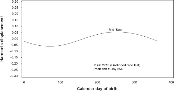
Calendar day of birth for peak risk of dying following diagnosis—unimodal fit (adjusted for period of birth and age).

Figure 2.

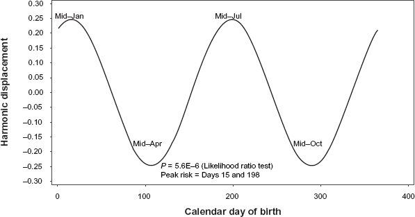
Calendar day for birth and peak risk of dying following diagnosis—bimodal fit (adjusted for period of birth and age).

Simulation Results

Using the SAS® programming language (version 9.2, Cary, NC), a simulation was performed to illustrate the relative efficiency of sinusoidal Cox regression compared with a traditional season-to-season Cox regression model. Sinusoidally varying observations, with the longest average survival times occurring among participants born during spring versus fall (ie, greatest risk of dying for fall births), were simulated as

\begin{matrix} survival_time = (10 + sqrt (50000) * abs \\ (rannor (501))) * ((0.33196 * \cos ((((floor (365 * \\ ranuni (714) + 1)) - 62) / 365) * 2 * arcos(- 1))) + 0.5; \end{matrix}

In the above code, rannor and ranuni are SAS® functions that generate values from a standard normal and uniform distribution, respectively. The numbers within the parenthesis for the functions denote random number generator seed values. The floor function returns the largest integer that is less than or equal to the argument and gives the day of birth.

A sinusoidal Cox regression model, as presented in this paper, was used to test the seasonality hypothesis that fall births were more likely to die sooner from disease than spring births. A season-to-season analysis involved comparing survival times among fall and spring (referent group) births by dummy coding season of birth (ie, fall = 1, spring = 0) as the independent variable in a Cox regression model.

The sinusoidal Cox regression model was observed to be relatively more efficient than the traditional season-to-season method at detecting a statistically significant season-of-birth effect, and efficiency improved as the number (n) of simulated survival time observations increased (Table 3). For example, for n = 35, the sinusoidal Cox model detected a significant season-of-birth effect on disease survival (P = 0.01491), whereas the season-to-season analysis failed to achieve a statistically significant result (P = 0.23593). A Kaplan-Meier plot (n = 200) contrasting survival curves for fall and spring births is shown in Fig. 3.

Table 3.

Comparison of sinusoidal and season-to-season Cox regression models.

Number of simulated survival time observations	Sinusoidal Cox regression model P value^†	Season-to-season Cox regression model (fall vs. spring) P value^†
35	0.01491	0.23593
45	0.00710	0.11987
50	0.00175	0.02745
100	1.05E-5	0.01103
150	5.21E-11	0.00021
200	1.57E-13	7.35E-6

Note:

†

Likelihood ratio test.

Figure 3.

Kaplan-Meier plot comparing survival times for fall and spring births (n = 200 simulated observations).

Discussion

We have presented a simple, iterative Cox regression-based method to analyze censored time-to-event outcome data with seasonal predictor variables. The method is a simple extension of earlier trigonometric models yet is easier to apply and interpret.^2529–30 A parallel sinusoidal logistic regression model has been presented in the literature for analyzing non-censored binary event data.²³

A useful feature of sinusoidal Cox regression is its ability to optimally fit a sinusoidal curve to the underlying data by plotting harmonic displacement against calendar time. Whereas no single method provides a universal approach to analyze harmonic data, the current method accommodates varying lengths of months, different populations at risk, simultaneous adjustment for multiple confounders, and it is reasonably robust when used for small samples. The accompanying statistical test will have greater family-wise power to detect a sinusoidal pattern than performing multiple pairwise seasonal or monthly comparisons.

Similar to a dose response relationship based upon a best-fitting monotonic model and a priori biologic mechanism of action, multiplicity correction is not necessary for the optimal peak sinusoidal Cox regression model. Additionally, the model takes into account consecutively high/low time periods (eg, order of events), and the definition of season does not depend on an arbitrary start and end date but rather is determined by the model algorithm.

Several potential limitations should be noted when interpreting the results of a sinusoidal Cox regression analysis. A discrepancy between values expected under the model and the actual data may result in biased parameter estimates. Accordingly, the data should be tested for goodness-of-fit using standard statistics methods for Cox regression.¹⁹ Ambiguous results may occur in the case of competing out-of-phase cycles resulting in a cancelling of effects (eg, opposing seasonally effects by hemisphere of birth). When appropriate, stratification or the use of a multimodal model may help mitigate this problem. Additionally, the sinusoidal Cox regression model as specified will not distinguish between major and minor peaks since the magnitude of harmonic displacement will be equal for all peaks.

A statistically insignificant seasonal risk factor in the model does not necessarily rule out an underlying seasonal effect. For example, the factor may a have lopsided shape that may be difficult to statistically detect using a sinusoidal Cox model. Conversely, the seasonal association of a specific risk factor with disease does not necessarily imply causality. As with any statistical model, the results of sinusoidal Cox regression should be carefully interpreted in light of underlying limitations and biologic plausibility. Furthermore, the lack of a well defined hypothesis in advance of analysis and selection bias may lead to spurious results. Selection bias generally is difficult to correct after the data have been collected. A type of selection bias based on differential survival of certain individuals in the population at risk is a particular concern in season-of-birth studies. For example, susceptible individuals with a weak immune system may die soon after birth and distort the population base of adult survival studies.

The example presented in this paper is limited in scope. Future studies would be needed to determine whether a bimodal peak of seasonal risk is unique to this data set. New studies also would benefit by adjusting for potential confounders such as tumor grade, gender, diet, and body weight, and stratifying analyses by hemisphere or latitude of birth. The sinusoidal Cox regression model will provide a flexible tool for conducting such analyses.

In summary, seasonal environmental exposures occurring within a brief “critical window” during prenatal development or early infancy have been hypothesized to influence susceptibility to disease and survival later in life..^31,32 Studies of season of birth and survival time have been difficult to interpret due to limitations of the statistical to methods used to analyze the data. In this paper, we have presented a sinusoidal Cox regression method that is derivative-free, easy to use, and it does not require the arbitrary demarcation of seasons characterizing other techniques. Furthermore, the sinusoidal Cox regression model yields a single P value, unlike traditional methods for analyzing seasonal data which require multiple pairwise comparisons. The sinusoidal model also is statistical more powerful in detecting season-of-birth trends in the data.

Disclosure

This manuscript has been read and approved by the author. This paper is unique and is not under consideration by any other publication and has not been published elsewhere. The author and peer reviewers of this paper report no conflicts of interest. The author confirms that they have permission to reproduce any copyrighted material.

Footnotes

Acknowledgements

The author thanks Dr. Katherine T. Jones for valuable comments during the writing of this manuscript and her knowledge and insight are greatly appreciated. The contents of this publication are solely the responsibility of the author and do not necessarily represent the views of any institution or funding agency.

Data File

STM	CDB	P	A	C	STM	CDB	P	A	C	STM	CDB	P	A	C	STM	CDB	P	A	C	STM
48	185	2	4	1	5	270	2	4	1	24	27	1	4	1	26	327	1	4	1	44
52	254	2	4	1	19	167	2	4	1	42	328	2	4	1	65	123	1	4	1	18
36	172	2	4	1	55	320	2	4	1	44	328	2	4	1	27	329	1	4	1	16
43	196	2	4	1	17	168	1	4	1	50	179	2	4	1	18	144	1	4	1	10
49	240	2	4	1	30	207	2	4	1	18	149	2	4	0	187	246	1	4	0	17
61	302	2	4	1	23	198	2	4	1	6	301	1	4	1	31	63	1	4	1	51
152	127	2	4	0	13	356	2	4	1	13	310	2	4	1	13	173	1	4	1	101
81	316	2	4	1	109	50	2	4	1	47	337	1	4	1	1	66	1	4	1	22
42	316	2	4	0	165	194	2	4	1	39	90	2	4	1	51	195	1	4	1	22
508	56	2	4	0	0	196	2	4	1	14	266	1	4	1	122	130	1	4	1	13
66	94	2	4	0	184	12	2	4	1	16	34	2	4	1	1	290	1	4	1	6
135	258	2	4	1	14	66	2	4	0	1	29	2	4	1	38	324	1	4	1	35
6	232	2	4	1	48	86	2	4	1	9	318	2	4	0	20	21	4	2	0	198
45	100	2	4	1	101	265	1	4	1	63	250	1	4	1	10	193	4	3	1	18
49	167	3	3	0	19	231	2	3	0	1008

Abbreviations: CDB, calendar day of the year birth date; P, period of birth (1 = 1917–29, 2 = 1930–39, 3 = 1940–49, 4 = 1950–59, 5 = 1960–69, 6 = 1970–79, 7 = 1980–89) A, age category (1 = ≤40 yrs., 2 = 41–50 yrs., 3 = 51–60 yrs., 4 = >60 yrs.); C, Censor variable (1 = dead, 0 = Alive); STM, survival time in weeks.

References

Muñoz-Tuduri

, Garcia-Moro

Season of birth affects short- and long-term survival.

Am J Anthropol. 2008; 135: 462–8.

Yamakawa

, Fukui

, Kinoshita

, Ohgami

, Kitamura

Seasonal variation in incidence of cerebellar medulloblastoma by month of birth.

Fukuoka Igaku Zasshi (Hukuoka Acta Medica). 1979; 70: 295–300.

Ederer

, Miller

, Scotto

, Bailer

Birth-month and infant cancer mortality.

Lancet. 1965; 7404: 185–6.

Meltzer

, Annegers

, Spitz

Month-of-birth and incidence of acute lymphoblastic leukemia in children.

Leuk Lymphoma. 1996; 23: 85–92.

Halperin

, Miranda

, Watson

, George

, Stanberry

Medulloblastoma and birth date: evaluating three US data sets.

Arch Environ Health. 2004; 59: 26–30.

Rice

, Ward

Age dependence of susceptibility to carcinogenesis in the nervous system.

Ann NY Acad Sci. 1982; 381: 274–89.

Alexandrov

, Aiello

, Rossi

Modifying factors in prenatal carcinogenesis.

In Vivo. 1990; 4: 327–36.

Druckrey

, Ivankovic

Teratogenic and carcinogenic effects in the offspring after single injection of ethylnitrosourea to pregnant rats.

Nature. 1966; 210: 1378–9.

Wechsler

, Kleihues

, Matsumoto

. Pathology of experimental neurogenic tumors chemically induced during prenatal and postnatal life. Ann NY Acad Sci. 1969; 159: 360–408.

10.

Sanders

Experimental carcinogenesis: induction of multiple tumors by viruses.

Cancer. 1977; 40: 1841–4.

11.

Efird

Season of birth and risk for adult onset glioma.

Int J Environ Res Public Health. 2010; 7: 1913–36.

12.

Bengtsson

, Lindström

Airborne infectious diseases during infancy and mortality in later life in southern Sweden, 1766–1894.

Int J Epidemiol. 2003; 32: 286–94.

13.

Cox

Regression models and life-tables (with discussion).

J R Stat Soc Ser B Stat (Methodological). 1972; 34: 187–220.

14.

Clark

, Bradburn

, Love

, Altman

Survival analysis part I: basic concepts and first analyses.

Br J Cancer. 2003; 89: 232–8.

15.

Bradburn

, Clark

, Love

, Altman

Survival analysis part II: multivariate data analysis—an introduction to concepts and methods.

Br J Cancer. 2003; 89: 431–6.

16.

Kelsey

, Whittemore

, Evans

, Thompson

Methods in Observational Epidemiology. New York: Oxford University Press, 1996: 1–412.

17.

Friedman

Primer of Epidemiology. New York: McGraw-Hill, 1994: 1–366.

18.

Spruance

, Reid

, Grace

, Samore

Hazard ratio in clinical trials.

Antimicrob Agents Chemother. 2004; 48: 2787–92.

19.

Allison

Survival Analysis Using the SAS System: A Practical Guide. Cary: SAS Institute, 1995: 1–292.

20.

Link

Confidence intervals for the survival function using Cox's proportional-hazard model with covariates.

Biometrics. 1984; 40: 601–10.

21.

Beckett

Personal communication (Harvard University). 1987.

22.

Chodick

, Shalev

, Goren

, Inskip

Seasonality in birth weight in Israel: new evidence suggests several global patterns and different etiologies.

Ann Epidemiol. 2007; 17: 440–6.

23.

Efird

, Searles Nielsen

A method to model season of birth as a surrogate environmental risk factor for disease.

Int J Environ Res Public Health. 2008; 5: 49–53.

24.

Efird

, Searles Nielsen

A method to compute multiplicity corrected confidence intervals for odds ratios and other relative effect estimates.

Int J Environ Res Public Health. 2008; 5: 394–8.

25.

Stutvoet

Seasonal birth frequencies in parameters.

Acta Genet Stat Med. 1951; 2: 177–92.

26.

Edwards

The recognition and estimation of cyclic trends.

Ann Hum Genet Lond. 1961; 25: 83–7.

27.

Thomas

, Wallis

Seasonal variation in regression analysis.

J R Statist Soc A. 1971; 134: 57–72.

28.

Roger

A significant test for cyclic trends in incidence data.

Biometrika. 1977; 64: 152–5.

29.

Stolwijk

, Straatman

, Zielhuis

Studying seasonality by using sine and cosine functions in regression analysis.

J Epidemiol Community Health. 1999; 53: 235–8.

30.

Haus

, Touitou

Chronobiology in laboratory medicine. In: Touitou

, Haus

, editors. Biological Rhythms in Clinical and Laboratory Medicine. Berlin and Heidelberg: Springer, 2001: 693–5.

31.

Ben-Shloma

, Kuh

Model advocates that an exposure in a critical period results in permanent and irreversible damage or disease.

Int J Epidemiol. 2002; 31: 285–93.

32.

Gillman

Epidemiological challenges in studying the fetal origins of adult chronic disease.

Int J Epidemiol. 2002; 31: 294–9.

Sinusoidal Cox Regression—A Rare Cancer Example

Abstract

Keywords

Introduction

Methodology

Example

Simulation Results

Discussion

Disclosure

Footnotes

Acknowledgements

Data File

References