Sage Journals: Discover world-class research

Abstract

Motivation

Existing methods for estimating copy number variations in array comparative genomic hybridization (aCGH) data are limited to estimations of the gain/loss of chromosome regions for single sample analysis. We propose the linear-median method for estimating shared copy numbers in DNA sequences across multiple samples, demonstrate its operating characteristics through simulations and applications to real cancer data, and compare it to two existing methods.

Results

Our proposed linear-median method has the power to estimate common changes that appear at isolated single probe positions or very short regions. Such changes are hard to detect by current methods. This new method shows a higher rate of true positives and a lower rate of false positives. The linear-median method is non-parametric and hence is more robust in estimating copy number. Additionally the linear-median method is easily computable for practical aCGH data sets compared to other copy number estimation methods.

Keywords

array CGH copy number alterations common copy number alterations regions

1. Introduction

During cell division, a cell replicates its genome by synthesizing a new copy of each chromosome, using the original DNA as a template. The expected copy number of 2, may be less/greater than 2 when alterations occur during the replication process. Research has suggested that such abnormalities in the number of DNA copies in a cell are associated with the development and progression of disease, including cancer.¹ Laboratory research to estimate the altered copy numbers in a DNA sequence often uses aCGH. The technology used to produce aCGH data, however, may result in data that contain uncontrollable noise.² The use of appropriate statistical methods to normalize the data and produce meaningful estimates of copy number variation in a DNA sequence is integral to this research. Developing improved statistical methods for this application is the focus of this paper.

Different statistical methods have been suggested for use with aCGH data to estimate copy numbers in DNA sequences. Methods to analyze copy numbers in terms of identifying the locations of gains or losses of chromosome regions have been developed. Assuming that there is a connection between copy number changes in a cancer cell and the development/progression of the cancer, there must exist some common change regions in DNA sequences collected from different patients with the same cancer diagnosis. Techniques for analyzing shared copy number regions have been developed..^3,4 For detecting copy number regions in a single sample, Olshen et al⁵ and Venkatraman et al⁶ had developed a widely used method, the faster circular binary segmentation (CBS) method. In this paper, we propose a new method, the linear-median method, for estimating shared copy number alterations in DNA sequences collected from the same type of cancer cells. The linear-median method is able to optimally use the information available across independent DNA sequences.

This paper is organized as follows. In Section 2.1, we discuss current existing statistical models used to assess aCGH data and describe a new model for analyzing multiple independent aCGH data sets. We introduce the linear-median method in Section 2.2. In Section 3.1, we present three simulation studies. We study how much extra information on copy number aberration can be obtained by using the linear-median method compared to the comparative genomic hybridization minimal common region (cghMCR) method and the CBS algorithm. We present an application of the linear-median method to real data in Section 3.2. Supporting figures and tables are available online as Supplementary Material.

2. Methods

2.1 Modeling DNA copy number alterations in aCGH data

aCGH employs the comparative hybridization of genomic DNA that is differentially labeled according to its source in a cancer cell versus a normal cell. The ratio of the hybridization intensities along the chromosomes provides a measure of the relative copy number of sequences in the genomes that hybridize to each location on the chromosomes. Estimating copy numbers and identifying the locations of gains and losses in a DNA sequence are two main challenges in the analysis of aCGH data. We label the normal genomic sequences as “reference” sample and the genomic sequences from cancer cells as the “test” sample. Let T_p denote the “test” copy number at probe position p and R_p denote the “reference” copy number at probe position p.

We briefly describe two current methods for modeling aCGH data. Let us denote by Y_p the aCGH data (the logarithm intensity ratio) observed at probe position p.

Model 1: $Y_{p} = \log_{2} (T_{p} / R_{p}) + ε_{p},$

Y_{p} = \log_{2} (T_{p} / R_{p}) + ε_{p},

(1)

where ∊_p are i.i.d. with normal distribution N(0, $N (0, σ_{ε}^{2})$ ). This Gaussian model forms the basis of many models for aCGH data.^4,6–8

Model 2:

Y_{p} = \log_{2} (\frac{T_{p} + ε_{p}}{R_{p} + η_{p}}),

(2)

where ∊_p and η_p are i.i.d with a normal distribution N(0,σ²)..^9,10

In practice, R_p is assumed to be 2. Given the logarithm intensity ratio observations, {Y_p}, we want to estimate the true copy number at position p or to estimate if the copy number at p is greater/less than 2.

Models 1 and 2 assume very different probability structures to describe the system. The variance of the log intensity ratios given by Model 1 is a constant, whereas the variance of the log intensity ratios given by Model 2 is a function of T_p.

We consider which of the two models is a more appropriate model for the analysis of aCGH data. Although Model 1 looks simpler, it is not an appropriate model for aCGH data. The main reason for this is that aCGH data provide the ratio of the copy number variations, not the ratio of the copy numbers. Furthermore, empirical studies show that the standard error of the logarithm of the intensity ratios increases as the copy number increases. Additionally, the distribution of the logarithm of intensity ratios is skewed.⁹ Thus, the distribution of ∊_p should not be assumed to be normal if Model 1 is adopted.

Compared to Model 1, Model 2 is a more appropriate model for aCGH data, as it takes into account the ratio of the copy number variations. However, this model can be improved further. The normality assumptions on the distributions of ∊_p and η_p can imply that negative values of ∊_p and η_p will lead to log₂ (T_p + ∊/2 + η) being ill-defined. Theoretically, this will cause problems for statistical inference methods based on such an assumption.

In Model 2, the errors ∊_p and η_p play the role of measurement errors. Given the fact that the aCGH technique is maturing, it might be reasonable to suggest that both ∊_p and η_p follow a uniform distribution U(–a, a), where a can assume any value between 0 and 2, depending on the nature of the underlying aCGH technique. If a takes a value close to 2, this may mean that the underlying aCGH technique is not very accurate, possibly leading to a very large variation in the observations of the intensity ratios. If a takes a value close to 0, we may assume that the underlying aCGH technique is very accurate and that there is less variation in the observations of the intensity ratios. For explicit technical considerations see wikipedia.² For our purpose, we restrict a to be less than 2. We apply this restriction to real data analysis in Section 3.2. The output of the real data analysis shows the restriction is acceptable.

Therefore, we consider a third model:

Model 3:

X_{p} = \frac{T_{p} + ε_{p}}{R_{p} + η_{p}},

(3)

where ∊_p and η_p are independent and have uniform distribution U(–a, a) with constant a ∈ (0, 2), and X_p is the observed intensity ratio at probe position p.

To allow the model to be more flexible, we can assume that the uniform distributions for ∊_p and η_p are not necessarily the same.

Model 3 is used to model one aCGH profile from one sample/patient. However, if there is a group of independent samples of aCGH data (eg, multiple patients) and their data share copy number change regions, we can extend Model 3 to such data.

Consider the following scenario. A group of n patients suffer from a common cancer. For each patient a sample of aCGH data is collected from a cancer cell. Let X_i,p be the observed intensity ratio for the ith sample at probe position p. We use t_p to denote the theoretical true value of the shared copy number at probe position p for the “test” and let T_i,p be the true copy number for the ith patient at probe position p. T_i,p is not necessarily equal to t_p because, for different patients, the copy number at position p might be affected by different uncontrollable random factors. We use T_p to denote the observed copy number for “test” at position p. T_p is a random variable and T_i,p is a sample from T_p. Let R_i,p be the true copy number for the ith “reference” at the position p. In this paper, we always assign R_i,p = 2 because the true copy number for the reference (normal) genome is 2 (For the purpose of this study we ignore some special cases).

For multiple independent aCGH data, the extended model can be considered as

Model 4:

\begin{array}{l} X_{i, p} = \frac{T_{i, p} + ε_{i, p}}{R_{i, p} + η_{i, p}}, \\ 1 \leq p \leq M, i = 1, 2, \dots, n, \end{array}

(4)

where M is the total number of probe positions; n is the number of independent samples in the group; ∊_i,p and η_i,p are mutually independent random variables; T_i,p has distribution P(T_i,p = t_p) = π and P(T_i,p = 2) = 1–π, if t_p ≠ 2, ie, if at probe position p the shared true copy number is not 2, then the copy number given by the ith sample at the probe position will follow a Bernoulli distribution with mean π; ∊_i,p and η_i,p will have uniform distributions U(–a,a), as defined in Model 3. (Different uniform distributions are allowed for ∊_i,p and η_i,p; however, such applications are beyond the scope of this paper.)

Model 4 provides a flexible way to model multiple independent aCGH data in terms of the following arguments:

The probability distributions of ∊_i,p and η_i,p are allowed to be different. This means that the probability distribution of the measurement errors for the “test” and “reference” are allowed to be different.

ii.

The true shared copy number at position p is no longer a constant. T_p is a random variable. This means that the copy number (if it were observable) at position p could be different from patient to patient.

Hereafter, we consider multiple independent aCGH data and assume Model 4 as the basis for developing a method to estimate the shared copy numbers t_p, p = 1, …, M.

2.2 The linear-median method

Currently, all raw data used for copy number analysis are presented in the format of a log₂ intensity of the ratios of the test to the reference. From the current literature, we know that a linear format refers to using the intensity of the ratios of the test to the reference, and a nonlinear format refers to using a log₂ intensity of the ratios of the test to the reference, as the log₂(ratio) is not linearly related to the copy number. The variance of a linear format tends to be larger than the variance of a nonlinear format when the relative copy number is far away from 1.¹¹ This may explain why the nonlinear format is widely used.

It is expected that the log₂ of the true relative copy number, ie, log₂(t_p/R_p), can be well estimated using the observations of the log₂ intensity of the ratios of the test to the reference, ie, log₂ [(T_i,p + ∊_i,p)/(R_i,p + η_i,p)], through the sample mean. Unfortunately, this is generally not true. A simple reason for this is that, in general,

\begin{array}{l} E [\log_{2} (\frac{T_{p} + ε_{p}}{R_{p} + η_{p}})] \neq \log_{2} (\frac{E [T_{p} + ε_{p}]}{E [R_{p} + η_{p}]}) \\ = \log_{2} (\frac{E [T_{p}]}{R_{p}}) . \end{array}

Further, the probability distribution of log₂[(T + ∊_p)/(R_p + η_p)] is not symmetric. Therefore, the sample mean of log₂ [(T_i,p + ∊_i,p)/(R_i,p + η_i,p)] might be biased from E [log₂ ((T_p +∊_p)/(R_p + η_p))] for smaller samples. Figure 1 shows a histogram of simulated data drawn from the population log₂ [(1 + ∊)/(2 + η)], with ∊ and η i.i.d. uniformly distributed U(–1.8, 1.8) (the function will not be defined if 1 + ∊ ≤ 0).

Figure 1.

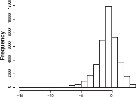
Histogram of log₂[(1 + ∊)/(2 + η)].

For the estimating procedure we propose, we will use linear format data rather than nonlinear format data to estimate the shared copy number at probe position p, 0 ≤ p ≤ M.

As defined in Model 4, X_i,p is a random variable of the intensity of the ratios of the test to the reference given by the ith sample at probe position p, 1 ≤ p ≤ M, and satisfies the model

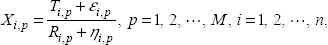
X_{i, p} = \frac{T_{i, p} + ε_{i, p}}{R_{i, p} + η_{i p}}, p = 1, 2, \dots, M, i = 1, 2, \dots, n,

where i denotes the ith sample/patient; ∊_i,p and η_i,p are i.i.d. with uniform distribution U(–a, a); T_i,p and R_i,p are the test intensity and reference intensity, respectively, for probe p for the ith sample.

As stated in Section 2.2, we always assign R_i,p = 2, which is the information given by the “reference” genome. The true shared copy number t_p at position p needs to be estimated. The estimate of t_p is denoted by ${\hat{t}}_{p}, 1 \leq p \leq M$ , 1 ≤ p ≤ M.

Let x_i,p be the observed values of X_i,p, i = 1, 2, …, n, p = 1, …, M. Herein, we assume that parameter a is unknown but has a value within (0, 2) and that parameter π (defined in Model 4) is known or can be estimated from empirical knowledge.

The estimation of t_p, p = 1, …, M, consists of three steps:

Step 1 Calculate the median of {x_i,p} _{i = 1,2, …,n} for each p, denoted by M_p.

Step 2 Calculate 2(M_p–1 + π)/π for each p.

Step 3 Determine the estimate of t_p, p = 1, …, M,

\begin{matrix} \begin{array}{l} {\hat{t}}_{p} = [2 (M_{p} - 1 + π) / π], if 2 (M_{p} - 1 + π) / π \\ \leq [2 (M_{p} - 1 + π) / π] + 0.5; \end{array} \\ \begin{array}{l} {\hat{t}}_{p} = [2 (M_{p} - 1 + π) / π] + 1, if 2 (M_{p} - 1 + π) / π \\ > [2 (M_{p} - 1 + π) / π] + 0.5; \end{array} \end{matrix}

where [c] denotes the integer part of the real number c.

We call this 3-step method the “linear-median method”. “Linear” indicates that the data (the intensity of the ratios of the test to the reference) are in a linear format. “Median” indicates that the median of the data is employed by this method.

Next, we explain theoretically why copy numbers can be accurately estimated by this 3-step method.

Let X_p be the intensity of the ratios of the test to the reference at probe position p,

X_{p} = \frac{T_{p} + ε_{p}}{2 + η_{p}},

where ∊_p and η_p are i.i.d. with uniform distribution U[–a, a); and T_p is a random variable independent of ∊_p and η_p, and has distribution P(T_p = t_p) = π and P(T_p = 2) = 1 – π, if the shared copy number t_p ≠ 2. As explained in Section 2.1, we assume 0 < a < 2.

Following the definition of X_p and assuming the independence of T_p + ∊_p and η_p, we have

\begin{matrix} E (X_{p}) = E (\frac{T_{p} + ε_{p}}{2 + η_{p}}) \\ = E (T_{p} + ε_{p}) E (\frac{1}{2 + η_{p}}) \\ = (t_{p} π + 2 (1 - π)) E (\frac{1}{2 + η}) \\ = \frac{t_{p} π + 2 (1 - π)}{2 a} \log (\frac{2 + a}{2 - a}) . \end{matrix}

Thus

t p = (\frac{2 a}{\log (\frac{2 + a}{2 - a})} E (X_{p}) - 2 (1 - π)) / π .

(5)

Equation (5) gives the exact relationship between t_p and E(X). For each probe position p, if the mean of the intensity of the ratios of the test to the reference is known, and the system parameters a and π are known, the shared copy number at the probe position can be correctly identified.

However, E(X_p) is unknown in practice and the probability distribution of X_p is not usually symmetric. It is inappropriate to estimate E(X_p) by using the sample mean ${\bar{X}}_{p}$ when the sample size is not appropriately large. Therefore, it is difficult to evaluate t_p directly from (5) in practice.

To overcome this difficulty, we suggest the following way to evaluate t_p:

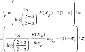
\begin{array}{l} t_{p} = (\frac{2 a}{\log (\frac{2 + a}{2 - a})} E (X_{p}) - 2 (1 - π)) / π \\ = (\frac{2 a}{\log (\frac{2 + a}{2 - a})} \frac{E (X_{p})}{m_{X_{p}}} m_{X_{p}} - 2 (1 - π)) / π, \end{array}

where $m_{X_{p}}$ is the median of X_p. It is technically possible to directly evaluate the ratio

\frac{a E (X_{p})}{\log (\frac{2 + a}{2 - a}) m_{X_{p}}}

(6)

and prove that the ratio is close to 1, for any a ∈ (0, 2) and any π ∈ (0, 1).

We use the Monte Carlo method to indirectly show that the value of (6) is close to 1 for a = 0.1, 0.2, …, 1.9 and π = 0.1, 0.2, …, 1. (see Appendix A and Supplementary Tables 1 and 2 in the online materials for details). Therefore,

t_{p} \approx \frac{2 (m_{X_{p}} - (1 - π))}{π} .

Table 1.

The sample mean and sample standard error of the estimated error rate {d(k)} given by different combinations of a and n, where a is the parameter of the uniform distribution U[–a, a] and n is the number of the independent sequences in the realizations.

a	n
	25	50	75
0.5	0.00267 (0.00505932)	0.00021 (0.00143456)	0.00003 (0.00054717)
0.8	0.03080 (0.01634096)	0.00578 (0.00725564)	0.00566 (0.01330000)
1	0.06900 (0.02388243)	0.01822 (0.01335702)	0.00771 (0.00880531)
1.5	0.19759 (0.03871163)	0.08208 (0.02652880)	0.04332 (0.02063500)
1.9	0.30161 (0.04409140)	0.15426 (0.03687835)	0.09367 (0.02802528)

Table 2.

Number of genes identified by the linear-median method (LM) and the cghMCR method in the regions of shared copy number aberrations with the status of copy number loss, neutrality or gain. NR/U is not cancer-related or unknown function phenotype, CR is cancer-related phenotype (except for lung cancer), and LCR is lung cancer-related phenotype.

	NR/U		CR		LCR		Total
	LM	cgh MCR	LM	cgh MCR	LM	cgh MCR	LM	cgh MCR
Losses	670	346	89	33	9	4	768	383
Neutral	342	758	35	103	3	9	380	870
Gains	100	8	13	1	1	0	114	9
	1112		137		13

3. Implementation and results

3.1 Simulation studies

The linear-median method is designed for estimating shared copy number aberrations and mainly focuses on the information across the sample for each probe position. Therefore, this method ignores the dependency within each individual sample. Our focus is two-fold: i) to determine the extent of information of shared copy number aberrations that can be detected, regardless of the impact of dependency, and ii) to assess the differences in detection outcomes obtained from the linear-median method versus other methods.

In a recent review of methods for detecting “recurrent” copy number alterations, Rueda and Diaz-Uriarte evaluated the CGHregions method, Master HMMs, cghMCR, GISTIC, MSA, RAE, and others.¹² In this subsection, we compare the linear-median method to the cghMCR method and the CBS method.

We present three simulation studies to highlight the performance of our proposed linear-median method.

Example 1: A sequence of integers serves as a sequence of the true shared copy number t_p, p = 1, 2, …, 100, obtained from the experimental sample, ie, the “test”. To simplify, we assume π = 1. Thus, for example, t₁ = 2 means that the true shared copy number shown by the “test” at probe position 1 is 2; t₁₁ = 3 means that the true gain in the shared copy number by the “test” at probe position 11 is 3.

2	2	2	2	2	2	2	2	2	2	3	3	3	3	3	3	3	3	3	3
2	3	3	3	3	3	3	3	3	3	2	2	2	2	2	2	2	2	2	2
1	1	1	1	1	2	2	2	2	2	3	3	3	3	3	4	4	4	4	4
5	5	5	5	5	2	2	2	2	2	2	2	2	2	2	3	3	3	3	3
1	1	1	1	1	3	3	3	3	3	2	2	2	2	2	2	2	2	2	2

We simulated a group of independent realizations {X_i,p} from model (t_p + ∊_i,p)/(2 + η_i,p), p = 1, 2, …, 100 and i = 1,2, …, n, where ∊_i,p and η_i,p are i.i.d. with uniform distribution U[–a, a].

Subsequently, we generated 1000 replicates. For the kth replicate, k = 1,2, …, 1000, let d(k) be the percentage of $t_{p} - {\hat{t}}_{p} \neq 0$ out of the 100 probe positions; d(k) is used to measure the error rate in the estimation of t_p. The mean and standard error of {d(k)} are presented in Table 1.

Table 1 shows that the error rate increases with a. This is obvious because a larger value of a is equivalent to a larger measurement error in the data. However, the error rate will be reduced when the number of independent samples in the group increases. In general, the mean error rate calculated for the linear-median method is reasonably low: the mean error rate was less than 10%, as expected, for all three cases of varying a.

Although the underlying model involves the parameter a, Example 1 shows, in general, that the impact of the value of a on the estimation of the copy number is not significant in terms of the mean of d(k), except for a very large value of a(>1). (Further demonstrations are presented in the Supplementary Material.) In summary, the value of a ∈ (0, 2) has minimal effect on the estimation of the shared copy number when the sample size is reasonable large. As a result, the linear-median method can be employed without knowing the value of a, as long as a ∈ (0, 2).

Example 2: In Table 1 of their review of 15 estimation methods, Rueda and Diaz-Uriarte indicate that only the cghMCR method both uses an input of the log2 ratio and produces estimations of the differences in the states of two successive probes.¹²

The cghMCR method is designed to identify the minimal common copy number alteration regions among a group of independent samples; thus it is analogous to the linear-median method and is an appropriate method to compare to the linear-median method. Using segmented data (ie, smoothed data), the cghMCR algorithm first identifies altered segments within each subject (those above the 97th or below the 3rd percentile of the data) and then joins adjacent segments separated by a user-defined parameter. The R package for the cghMCR method is available at the following URL: http://www.bioconductor.org/packages/2.6/bioc/html/cghMCR.html. See the work of Aguirre et al for explicit details and a complete review of the cghMCR method.³

We use simulated data to compare the performance of the linear-median method to that of the cghMCR method. The data were simulated by assuming non dependency between the intensity ratios across probe positions, which is a very simple situation.

Consider a sequence of true shared copy number {t_p} plotted in Figure 2.

Figure 2.

Plot of the sequence of the true copy numbers.

The sequence t_p consists of four abnormal shared copy number regions, corresponding to copy numbers 1, 3, 4 and 5. Some of the abnormal shared copy regions are very short, involving only 1 or 4 probe positions. Using this example, we compare the linear-median method to the cghMCR method in terms of each methods’ capability of correctly assessing the information of gains/losses in shared copy numbers.

We simulated data from the following model

X_{i, p} = {\begin{matrix} \frac{2 + ε_{i, p}}{2 + η_{i, p}}, & 1 \leq p \leq 10, \\ \frac{B {(1, π)}_{i, p} + 2 (B {(1, π)}_{i, p} - 1) + ε_{i, p}}{2 + η_{i, p}}, & 11 \leq p \leq 50, \\ \frac{2 + ε_{i, p}}{2 + η_{i, p}}, & 51 \leq p \leq 98, \\ \frac{4 B {(1, π)}_{i, p} + 2 (B {(1, π)}_{i, p} - 1) + ε_{i, p}}{2 + η_{i, p}}, & 99 \leq p \leq 102, \\ \frac{2 + ε_{i, p}}{2 + η_{i, p}}, & 103 \leq p \leq 109, \\ \frac{5 B {(1, π)}_{i, p} + 2 (B {(1, π)}_{i, p} - 1) + ε_{i, p}}{2 + η_{i, p}}, & p = 110, \\ \frac{2 + ε_{i, p}}{2 + η_{i, p}}, & 111 \leq p \leq 150, \\ \frac{3 B {(1, π)}_{i, p} + 2 (B {(1, π)}_{i, p} - 1) + ε_{i, p}}{2 + η_{i, p}}, & 151 \leq p \leq 200, \\ \frac{2 + ε_{i, p}}{2 + η_{i, p}}, & 201 \leq p \leq 250, \end{matrix}

(7)

i = 1, 2, …, n, where ∊_i,p, and η_i,p are i.i.d. with uniform distribution U(–a, a). Let B(1, π) be a random variable with a Bernoulli distribution such that E[B(1, π)] = π. We considered 3 × 5 × 3 different combinations for (a, π, n), where a = 0.5, 1, 1.5, π = 0.2, 0.4, 0.6, 0.8, 1 and n = 20, 50, 100.

We applied the linear-median method and the cghMCR method to each group of independent samples with size n for different pairs of parameters (a, π), respectively. Then, for each triplet (a, π, n), we calculated the true positive (TP) rates and the false positive (FP) rates produced by each model. TP rate = P(the method shows “copy number changed” | copy number is changed). FP rate = P(the method shows “copy number changed” | copy number is not changed). The linear-median method is able to provide an estimate of the shared copy number at each probe position. Therefore, when we say that a correct detection of the shared copy number was produced by the linear-median method at position p, it means that ${\hat{t}}_{p} = t_{p}$ . In contrast, the cghMCR method provides information on only the shared copy number gain/loss at each probe position. It does not provide information on how many copy numbers were gained/lost. Therefore, when we say that a correct detection was produced by the cghMCR method at position p, it means only that a gain/loss was correctly identified at position p.

Finally, we carried out 250 replicates for the case where n = 20; 100 replicates for the case where n = 50, and 50 replicates for the case where n = 100. The resulting TP and FP rates, means, and standard errors obtained from both methods are shown in Supplementary Tables 3–5.

Table 3.

List of lung cancer-related genes for each phenotypic group identified by the linear-median method (LM) and the cghMCR method.

	LM	cghMCR
Loss	PSIP1, CDKN2A TUSC1, IGFBPL1 TLE1, FRMD3 DAPK1, MIRLET7A1 PTPN3	PSIP1, CDKN2A TUSC1, IGFBPL1
Neutral	PHF19, DAB2IP RPL12	PHF19, DAB2IP RPL12, TLE1 FRMD3, DAPK1 MIRLET7A1, PTPN3 GAS1
Gain	GAS1

In terms of the TP rates, the linear-median method worked reasonably well in each case and performed vastly better than the cghMCR method, which showed poor performance, especially when a was larger and π was smaller. In this particular example of a true shared copy number sequence, the cghMCR method tended to give a lower FP value, ie, it did not call as many gains/losses, and hence was very conservative. Compared to the cghMCR method, the linear-median method gave a lower FP value when a was not close to 2 or π was greater than 0.5. In summary, two advantages of using the linear-median method include:

The ability to estimate the actual shared copy number at each position p. The estimation accuracy of the linear-median method is very high, as reflected by the values of the TP and FP rates.

Better power in identifying shorter alternating regions. For example, considering the data simulated from (7) with a = 1.5, π = 1 and n = 20, we can compare the means of the estimated copy numbers given by both methods. Since a = 1.5, the variance for U(–a, a) is relatively large and the simulated data involve a lot of random noise. By choosing π = 1, there is no variation on the true copy numbers shared across the independent samples. Technically, one expects that the linear-median method and the cghMCR method will perform at the same level. However, it turns out that the linear-median method dominates the cghMCR method. 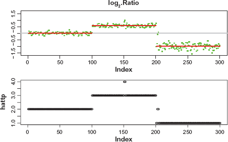At almost every probe position, the sample mean and median of the estimated shared copy number given by the linear-median method was the same as the true shared copy number. In contrast, the cghMCR method did not accurately identify the gain/loss regions (see Supplementary Figures 1–3).

Figure 3.

Application of the CBS method to the sequence of the median of the logarithm of the ratios (top panel). The red bars show the values of the estimation of log₂(t_p/2). Application of the linear-median method to the data in Example 3 (bottom panel), showing the estimates of t_p at each probe position.

This simulation example (Example 2) illustrates that the cghMCR method performs very poorly in high-noise scenarios, for example, a = 1.5, and the cghMCR method is not robust for large values of a. We believe this is due to the fact that the cghMCR method performs segmentation and calling functions independently of one other; whereas the linear-median method borrows strength from all the samples.

Example 3: In this example we consider data X_i,p, simulated from the following model:

X_{i, p} = \frac{t_{p} + ε_{i, p}}{2 + η_{i, p}} = {\begin{matrix} \frac{2 + ε_{i, p}}{2 + η_{i, p}} & 1 \leq p \leq 100, & l = 100 \\ \frac{3 + ε_{i, p}}{2 + η_{i, p}} & 101 \leq p \leq 150, & l = 50 \\ \frac{4 + ε_{i, p}}{2 + η_{i, p}} & 151 \leq p \leq 152, & l = 2 \\ \frac{3 + ε_{i, p}}{2 + η_{i, p}} & 153 \leq p \leq 200, & l = 48 \\ \frac{1 + ε_{i, p}}{2 + η_{i, p}} & 201 \leq p \leq 202, & l = 2 \\ \frac{2 + ε_{i, p}}{2 + η_{i, p}} & 203 \leq p \leq 204, & l = 2 \\ \frac{1 + ε_{i, p}}{2 + η_{i, p}} & 205 \leq p \leq 300, & l = 96 \end{matrix}

where ∊_i,p, and η_i,p, are i.i.d uniformly distributed in [–1, 1], i = 1, 2, … 60. In this example we continue to assume π = 1. The abnormal copy number regions are [101, 150] for t_p = 3; [151, 152] for t_p = 4; [153, 200] for t_p = 3; [201, 202] and [205, 300] for t_p = 1. Segments of [101, 150], [153, 200] and [205, 300] are relatively longer. Segments of [151, 152] and [201, 202] are relatively shorter.

In this example, we compare the linear-median method to the circular binary segmentation (CBS) method, which was developed by Olshen et al.⁶ An R package description for the CBS method is available at the following URL: http://bioconductor.org/packages/2.6/bioc/manuals/DNAcopy/man/DNAcopy.pdf. The CBS method is employed to find segments along the chromosome that share constant DNA copy numbers. Technically, it is inappropriate to directly compare the analytical results obtained by these two methods because the CBS method is designed for application to a single sample of data, whereas the linear-median method is applicable to a group of independent samples.

To apply the CBS algorithm to observations {x_i,p}, i = 1, …, 60, p = 1, …, 300, we make the following adjustment. We calculate log₂(x_i,p) for all i and p, since the CBS method is designed for data in a nonlinear format. Then, for each fixed p, we calculate the median of {log₂(x_i,p)}, forming a new sequence. Finally, we apply the CBS method to this sequence. We justify this comparison with the following argument: If there are common copy number alteration regions among the group of independent samples, the new sequence must contain the information on shared common regions. We consider the new sequence as if it were a single sample of data from a “patient”. Thus, if the information of a shared common region is strong enough, the CBS method should be able to detect the region based on the data of the new sequence. We used the default parameters in our application of the R package to the simulation data in this example.

Figure 3 shows the plot of the medians of {log₂(x_i,p)} and the estimate of log₂(t_p/2) (in red), obtained by the CBS method (top panel), and the plot of the estimation of t_p obtained by the linear-median method (bottom panel). We see that the linear-median method is able to detect all the changes in the copy number.

Comparing the plots in Figures 3, both approaches, the linear-median method and the CBS method, were able to detect all the longer regions of alternations. However, all the shorter regions of alterations, [151, 152], [201, 202] and [203, 204], were missed by the CBS method. This indicates that the linear-median method has more power than the CBS method to detect shorter segments of alterations or narrow gaps between segments.

3.2 Application to real data

We applied the linear-median method to a subset of aCGH data from 39 well-studied lung cancer cell lines.

The data, originally published by Coe et al¹³ and Garnis et al¹⁴ are available for downloading from http://sigma.bccrc.ca/. For this study, we used data from only the subgroup with the largest sample size, that of non-small cell adenocarcinoma (NA), which included 18 samples.

As both the linear-median method and the cghMCR method are designed for application to multiple aCGH data, the sample size is a critical issue. Data with more independent samples are able to provide more information on the commonalities across all samples.

Accurately identifying the locations of copy number aberrations has many important medical applications. As far as we know, the cghMCR method is one of the methods used to estimate the shared copy number for multiple aCGH data. Many other methods give an estimation of only the probability of gain/loss at each probe position..^4,13

Information on the exact shared copy number(s) at each probe position is not available for the data we have analyzed (the NA data). Therefore, based on only the analytic outputs of the linear-median method and the cghMCR method, it is difficult for us to claim which method is better in terms of the accuracy of estimating the true copy numbers. As a result, we compared the similarities between the analytic outputs of the two methods and determined which method provides more information on the changes in the copy numbers in the NA data. As a reference for this comparison, we used the probability of gain/loss at each probe position that was reported by Shah et al.⁴

The total number of probe positions in the NA data (chromosome 9) is 1249. Recalling Model 4 in Section 2.1, in order to estimate the shared copy numbers in a “test” DNA sequence, we need to know the parameter π. This type of information is also required for the cghMCR method. The value of π might be estimated based on the researcher's empirical knowledge. For the NA data, empirical knowledge on the value of π is not available. Therefore, we applied the cghMCR method and the linear-median method to the data for different values of π, 0.2, 0.4, 0.6, 0.8 and 1. Then we compared the results from both methods and also compared those results to findings reported by Shah et al.⁴ We expected to find little difference in the results obtained from the three methods. Shah et al found a loss of the shared copy number in a significant portion of the NA data (see Figure 7 in their paper).⁴ However, for π = 0.4, 0.6, 0.8 or 1, both the cghMCR method and the linear-median method provided high proportions of neutral states, ie, where the shared copy number equals 2. Therefore, it is reasonable to use π = 0.2 when analyzing the NA data. We limit our report of the analytic results to the case where π = 0.2.

Combining all the results given by the linear-median method and the cghMCR method for π = 0.2, 0.4, 0.6, 0.8 and 1, we were able to identify a common trend in the outputs of the two methods for all probe positions as the value π moves from 1 to 0.2 (data not shown). For the NA data, both the linear-median method and the cghMCR method give neutral states to all probe positions when π is assigned as 1, with the exception of a few probe positions identified as gain/loss by the linear-median method. In our empirical study of the NA data, if a probe position a is more likely to lose copy number(s), then the shared copy number estimation given by both methods will decrease as π moves from 1 to 0.2; if a probe position a is more likely to gain copy number(s), then the shared copy number estimation given by both methods will increase as π moves from 1 to 0.2. One important phenomenon we observed from the outputs of the two methods is that once a probe position has been identified as having a shared copy number change when π = π₀, the observation remains the same for any π > π₀. Comparing the results of the two methods, we found that the estimation of the shared copy number at each probe position given by the cghMCR method is reluctant to change as the value of π decreases. In contrast, the linear-median method can show changes in the estimated shared copy number as π decreases. This may reflect the later detection of an aberration by the cghMCR method compared to the linear-median method when the true shared copy number at a probe position is gained/lost, and as the value of π decreases. Based on our analysis of the NA data, the linear-median method was able to report the estimated shared copy number at each probe position; whereas the cghMCR method reported only the state of the shared copy number, ie, wether there was a gain, loss or no change (neutral state), in the shared copy number. To simplify the comparison between the results given by the two methods, we report only the gain, loss, or neutral states of the shared copy number for the linear-median method. A plot of the states for both methods is given in Figure 4. In the plot, we use “1”, “0” and “–1” to indicate a shared copy number gain, neutrality, or loss, respectively. We summarize the results as follows.

Figure 4.

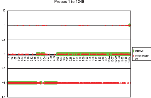
The output of the linear-median adjusted method is shown in red and that of the cghMCR method is in green.

From probe positions 1 to 500 and 1235 to 1249, both the cghMCR method and the linear-median method provide similar results, except for some isolated prob positions. This is what we expect to find because our simulation studies demonstrated that the linear-median method can identify those isolated regions.

From probe positions 501 to 1234, the results obtained from the linear-median method and the cghMCR method are quite different. The cghMCR method claims that all the probe positions are neutral, in contrast to the findings of the linear-median method, which identifies gains/losses at these probe positions. One possible explanation for the large difference between the two sets of results in this prob region is that the π used in the estimation for this region may be too high. A lower value of π should be used to accurately estimate copy numbers in this interval. These results suggest that the parameter π might vary over sequences of NA data. If this is true, then, detecting the change in π will be an interesting challenge for future studies.

Information on the true shared copy numbers for the NA data is not available; hence, we cannot be certain which method would best estimate the shared copy number variations in these data. However, through our comparison of the two methods and taking into account the results given by Shah et al⁴ we can claim that the linear-median method has some capability to reasonably estimate shared copy numbers in DNA sequences. As shown in our simulation studies, the linear-median method can easily identify isolated probe positions with shared copy number changes or short shared alternating segments. These changes are often missed by the cghMCR approach.

The 1249 probe sets we studied target the shared copy number status of 1262 genes present in the chromosome 9.

In order to classify these genes as one of three general categories, we performed a search of the OMIM database (http://www.ncbi.nlm.nih.gov/omim). The three categories we used were “not related to/unknown cancer phenotype (NR/U)”, “cancer-related phenotype, except for lung cancer (CR)”, and “lung cancer-related phenotype (LCR)”. The results are presented in Tables 2 and 3. Identifying altered regions where important cancer-related genes are located aids the biological interpretation of our findings and works as an empirical form of validation. Detailed locations of the genes categorized as NR/U, CR and LCR are presented in Supplementary Appendix B. From Tables 2 and 3 we can see that the linear-median method is able to report more CR and LCR with copy number losses/gains than the cghMCR method.

We were able to find additional information of interest from the output of the linear-median method. Focusing on the probe positions at which the estimated shared copy number given by the linear-median method was <1 or >3 when π = 0.2, we identified 145 such probe positions out of 1249 (see Figure 5). Among those 145 probe positions, 22 probe positions showed an estimated copy number ≥4 or ≤–1. These results provided a more serious warning of copy number aberrations — a warning that was not obtained from the cghMCR method.

Figure 5.

The plot of the estimated copy numbers (<1 or >3) given by the linear-median method for π = 0.2.

4. Conclusion

We developed a new model for aCGH data analysis, the linear-median method, which estimates shared copy numbers in DNA sequences. Using simulated data, we found the linear-median method to be more powerful than the cghMCR method in terms of achieving a higher rate of true positives and a lower rate of false positives. In addition to estimating the common gain/loss of chromosome regions, the linear-median method estimates the number of DNA copies. In other words, analytic results produced by the linear-median method allow us to extract additional information on the tested DNA sequences. In particular, the linear-median method has the power to estimate common changes that appear at isolated single probe positions or very short regions. The only drawback of the linear-median method is that it ignores the dependency information in samples. However, based on our application of the proposed method to real data, we find that most information on shared copy number aberrations can be captured by the linear-median method using only the information across independent samples.

Disclosure

This manuscript has been read and approved by all authors. This paper is unique and is not under consideration by any other publication and has not been published elsewhere. The authors and peer reviewers of this paper report no conflicts of interest. The authors confirm that they have permission to reproduce any copyrighted material.

Footnotes

Acknowledgement

V. Baladandayuthapani was partially supported by US National Science Foundation grant IIS 0914861. K.-A. Do was partially supported by the University of Texas SPORE grants in Prostate Cancer P50 CA140388, Breast Cancer P50 CA116199, Brain Cancer P50 CA127001, and the Cancer Center Support Grant P30 CA016672. We would also like to acknowledge LeeAnn Chastain (UTMDACC) for her editorial contributions to the manuscript.

Supplementary Material Appendix A

Use Monte Carlo method to indirectly show that the value of aE(X_p)/{log[(2+a)/(2–a)]m_Xp} is close to 1 for a = 0.1, 0.2,…, 1.9 and π = 0.1, 0.2, …, 1.

The simulation is conducted as follows. For each triplet (a, π, t_p), 5000 independent samples are simulated from model

where random variables T_p, ∊ and η are independent; T_p has a distribution such that P(T_p = t_p) = π and P(T_p = 2) = 1 – π; ∊ and η have uniform distribution U(–a, a), a = 0.1, 0.2, 0.3, …, 1.9 and π = 0.1, …, 1 with increments of 0.1 respectively; t_p = 1, 2, …, 9 with increments of 1. The mean and median of X_p(a, π) are estimated by its sample mean ${\bar{X}}_{p} (a, π)$ (a, π) and sample median median(X_p)(a, π) respectively. Then aE(X_p(a,π))/{log[(2+a)/(2–a)] m_Xp(a,π)} is estimated and evaluated by

For each π and t_p fixed, the sample mean m(π, t_p) and sample variance s²(π, t_p) of

are calculated by the following formulae:

and reported in Tables 1 and 2, which follow, where s²(π) is given within the parentheses.

The Monte Carlo simulation results clearly show that all the sample means m(π, t_p) are close to 1 and the sample variance s²(π, t_p) are close to 0. Therefore, it is reasonable to accept that aE(X_p(a,π))/{log[(2+a)/(2–a)] m_Xp(a,π)}, for any a ∈ (0, 2), π ∈ (0, 1) and t_p ∈ {1, …, 9}.

Appendix B

The locations of the genes of NR/U, CR and LCR in non-small cell adenocarci-noma (NA) and related references.

R code for the linear-median function

Table S5.

The true positive (TP) rates and false positive (FP) rates for the linear-median method and the cghMCR method, where n = 100.

n = 100	L-M	cgh MCR	L-M	cgh MCR	L-M	cgh MCR
π	α = 0.5		α = 1		α = 1.5
0.2
TP	0.6771 (0.0539)	0.0048 (0.0203)	0.7438 (0.0505)	0 (0)	0.7335 (0.0461)	0 (0)
FP	0.0561 (0.0187)	0 (0)	0.3266 (0.0412)	0 (0)	0.5146 (0.0381)	0 (0)
0.4
TP	0.9566 (0.0233)	0.6650 (0.1317)	0.9299 (0.02653)	0.0004 (0.0030)	0.8718 (0.0341)	0 (0)
FP	0.0003 (0.0013)	0.0455 (0.0270)	0.0578 (0.0196)	0 (0)	0.2012 (0.0340)	0 (0)
0.6
TP	0.9998 (0.0015)	0.9033 (0.0108)	0.9920 (0.01010)	02804 (0.0706)	0.9556 (0.0239)	0 (0)
FP	0 (0)	0 (0)	0.0065 (0.0075)	0 (0)	0.0621 (0.0224)	0 (0)
0.8
TP	1 (0)	0.8956 (0.0087)	0.9998 (0.0015)	0.3345 (0.0193)	0.9922 (0.0099)	0 (0)
FP	0 (0)	0 (0)	0.0003 (0.0013)	0 (0)	0.0167 (0.0125)	0 (0)
1
TP	1 (0)	0.8971 (0.0177)	0.9998 (0.0015)	0.2263 (0.1156)	0.9983 (0.0044)	0 (0)
FP	0 (0)	0 (0)	0.0003 (0.0013)	0 (0)	0.0043 (0.0056)	0 (0)

References

Cappuzzo

, Hirsch

F.R.

, Rossi

. Epidermal growth factor receptor gene and protein and gefitinib sensitivity in non-small-cell lung cancer. J Nat Cancer Inst. 2005; 97: 643–55.

http://en.wikipedia.org/wiki/Array_comparative_genomic_hybridization

Aguirre

A.J.

, Brennan

, Bailey

. High-resolution characterization of the pancreatic adenocarcinoma genome. Proc Nat Acad Sci U S A. 2004; 101: 9067–72.

Shah

S.P.

, Xuan

, deLeeuw

R.J.

. Integrating copy number polymorphisms into array CGH analysis using a robust HMM. Bioinformatics. 2006; 22: e431–9.

Venkatraman

E.S.

, Olshen

A.B.

A faster circular binary segmentation algorithm for the analysis of array CGH data.

Bioinformatics. 2007; 23: 657–63.

Olshen

A.B.

, Venkatraman

E.S.

, Lucito

, Wigler

Circular binary Segmentation for the analysis of array-based DNA copy number data.

Bio Statistics. 2004; 5: 557–72.

Molinaro

A.M.

, van der Laan

M.J.

, Moore

D.H.

Comparative Genomic Hybridization Array Analysis. U.C. Berkeley Division of Bio-statistics Working Paper Series. Working Paper Series. Working Paper 106. http://www.bepress.com/ucbbiostat/paper106. 2002.

Guha

, Li

, Neuberg

Bayesian hidden Markov modeling of array CGH data.

J Am Stat Assoc. 2008; 103: 485–97.

Pinkel

, Albertson

D.G.

Comparative genomic hybridization.

Ann Rev Genom Hum Genet. 2005; 6: 331–54.

10.

Pinkel

, Albertson

D.G.

Array comparative genemic hybrization and its application in cancer.

Nat Genet. 2005; 37 Suppl: S11–7.

11.

Pinkel

, Davis

, Albertson

Detection of gene dosage abnormalities using comparative genomic hybridization. http://cancer.ucsf.edu/array/nccls_pinkel.pdf. 2005.

12.

Rueda

O.M.

, Diaz-Uriarte

Finding recurrent copy number alteration regions: a review of methods.

Current Bioinformatics. 2010; 5: 1–17.

13.

Coe

B.P.

, Lockwood

W.W.

, Girard

. Differential disruption of cell cycle pathways in small cell and non-small cell lung cancer. Br J Cancer. 2006; 94: 1927–35.

14.

Garnis

, Lockwood

W.W.

, Vucic

. High resolution analysis of non-small cell lung cancer cell lines by whole genome tiling path array CGH. Int J Cancer. 2006; 118: 1556–64.

15.

Kamb

, Gruis

N.A.

, Weaver-Feldhaus

. A cell cycle regulator potentially involved in genesis of many tumor types. Science. 1994; 264: 436–40.

16.

Singh

D.P.

, Kimura

, Chylack

L.T.

Jr , Shinohara

Lens epithelium-derived growth factor (LEDGF/p75) and p52 are derived from a single gene by alternative splicing.

Gene. 2000; 242: 265–73.

17.

Shan

, Parker

, Wiest

J.S.

Identifying novel homozygous deletions by microsatellite analysis and characterization of tumor suppressor candidate 1 gene, TUSC1, on chromosome 9p in human lung cancer.

Oncogene. 2004; 23: 6612–20.

18.

Cai

, Chen

H.T.

, Boyle

, Rupp

, Funk

W.D.

, Dedera

D.A.

Identification of a novel insulin-like growth factor binding protein gene homologue with tumor suppressor like properties.

Biochem Biophys Res Commun. 2005; 331: 261–6.

19.

Allen

, van Tuyl

, Iyengar

. Grg1 acts as a lung-specific oncogene in a transgenic mouse model. Cancer Res. 2006; 66: 1294–301

20.

Haase

, Meister

, Muley

. FRMD3, a novel putative tumour suppressor in NSCLC. Oncogene. 2007; 26: 4464–8.

21.

Inbal

, Cohen

, Polak-Charcon

. DAP kinase links the control of apoptosis to metastasis. Nature. 1997; 390: 180–4.

22.

Johnson

S.M.

, Grosshans

, Shingara

, Byrom

, Jarvis

, Cheng

. RAS Is Regulated by the let-7 MicroRNA Family. Cell. 2005; 120: 635C647.

23.

Gobeil

, Zhu

, Doillon

C.J.

, Green1

M.R.

A genome-wide shRNA screen identifies GAS1 as a novel melanoma metastasis suppressor gene.

Genes Dev. 2008; 22: 2932–40.

24.

Wang

, Shen

, Parsons

D.W.

. Mutational analysis of the tyrosine phosphatome in colorectal cancers. Science. 2004; 304: 1164–6.

25.

Yano

, Toyooka

, Tsukuda

. Aberrant promoter methylation of human DAB2 interactive protein (hDAB2IP) gene in lung cancers. Int J Cancer. 2005; 113: 59–66

26.

Cuccurese

, Russo

, Pietropaolo

Alternative splicing and nonsense-mediated mRNA decay regulate mammalian ribosomal gene expression.

Nucleic Acids Research. 2005; 33: 5965–77.

2	2	2	2	2	2	2	2	2	2	3	3	3	3	3	3	3	3	3	3
2	3	3	3	3	3	3	3	3	3	2	2	2	2	2	2	2	2	2	2
1	1	1	1	1	2	2	2	2	2	3	3	3	3	3	4	4	4	4	4
5	5	5	5	5	2	2	2	2	2	2	2	2	2	2	3	3	3	3	3
1	1	1	1	1	3	3	3	3	3	2	2	2	2	2	2	2	2	2	2

2	2	2	2	2	2	2	2	2	2	3	3	3	3	3	3	3	3	3	3
2	3	3	3	3	3	3	3	3	3	2	2	2	2	2	2	2	2	2	2
1	1	1	1	1	2	2	2	2	2	3	3	3	3	3	4	4	4	4	4
5	5	5	5	5	2	2	2	2	2	2	2	2	2	2	3	3	3	3	3
1	1	1	1	1	3	3	3	3	3	2	2	2	2	2	2	2	2	2	2

Estimating Shared Copy Number Aberrations for Array CGH Data: The Linear-Median Method

Abstract

Motivation

Results

Keywords

1. Introduction

2. Methods

2.1 Modeling DNA copy number alterations in aCGH data

3.1 Simulation studies

Disclosure

Footnotes

Acknowledgement

Supplementary Material Appendix A

Appendix B

R code for the linear-median function

References

2	2	2	2	2	2	2	2	2	2	3	3	3	3	3	3	3	3	3	3
2	3	3	3	3	3	3	3	3	3	2	2	2	2	2	2	2	2	2	2
1	1	1	1	1	2	2	2	2	2	3	3	3	3	3	4	4	4	4	4
5	5	5	5	5	2	2	2	2	2	2	2	2	2	2	3	3	3	3	3
1	1	1	1	1	3	3	3	3	3	2	2	2	2	2	2	2	2	2	2