High-Dimensional Statistical Learning: Roots,Justifications,and Potential Machineries

Abstract

High-dimensional data generally refer to data in which the number of variables is larger than the sample size. Analyzing such datasets poses great challenges for classical statistical learning because the finite-sample performance of methods developed within classical statistical learning does not live up to classical asymptotic premises in which the sample size unboundedly grows for a fixed dimensionality of observations. Much work has been done in developing mathematical-statistical techniques for analyzing high-dimensional data. Despite remarkable progress in this field, many practitioners still utilize classical methods for analyzing such datasets. This state of affairs can be attributed, in part, to a lack of knowledge and, in part, to the ready-to-use computational and statistical software packages that are well developed for classical techniques. Moreover, many scientists working in a specific field of high-dimensional statistical learning are either not aware of other existing machineries in the field or are not willing to try them out. The primary goal in this work is to bring together various machineries of high-dimensional analysis, give an overview of the important results, and present the operating conditions upon which they are grounded. When appropriate, readers are referred to relevant review articles for more information on a specific subject.

Introduction

Classical statistical techniques have been fashioned for situations in which the number of data points is much larger than the number of variables. ¹ This is in large part due to the classical notion of statistical consistency, which guarantees the performance of a statistical technique in situations where the number of measurements unboundedly increases (n ↠ ∞) for a fixed dimensionality p of observations.^2–5

However, even though many modern datasets are characterized by a number of variables far exceeding the sample size, many practitioners still utilize classical learning methods to extract information out of such datasets. This state of affairs can be attributed, in part, to a lack of knowledge and, in part, to the ready-to-use computational and statistical software packages that are well developed for classical techniques. Nonetheless, one may argue that the so-called curse of dimensionality phenomenon in statistical learning can serve as a justification for utilizing classical techniques, and no need exists to incorporate many variables in a model. This phenomenon states that, when one attempts to improve performance by increasing the number of variables for a given number of data points, the performance improves up to a certain point, after which it starts deteriorating. ⁶ This phenomenon seems a justification for reducing the number of variables (dimensionality reduction) to a small number, perhaps much less than the sample size. In this reduced feature space, we are then “safe” to apply classical schemes because now the sample size is potentially much larger than the number of variables. The effect of the curse of dimensionality and its implications will be described in more detail later.

Using classification as an archetype, the dimensionality reduction generally follows a common methodology: 1) use a classification rule, including a feature selection, to design a classifier, and 2) use an error estimation rule to estimate the error of the designed classifier. The performance of many widely used classifiers is guaranteed in situations where n » p. They are designed to converge (in probability) to the Bayes classifier (optimal classifier) if n ↠ ∞ and p is fixed. Likewise, the performance of many error estimation rules lives up to similar asymptotic premises. Therefore, the feature selection strategy serves as an interface in order to scale the complexity of data to one that can be studied through classical methods. Fortunately, two mathematical-statistical machineries exist that are specifically designed to serve in high-dimensional settings: 1) shrinkage, and 2) the Girko G-analysis. These frameworks can serve as potential machineries in order to develop mathematical models suitable for analysis in situations where in the dimensionality of observations is comparable or potentially larger than the sample size. While the shrinkage estimation is grounded on the sparsity principle, G-analysis, in its simplest form, is based on double asymptotics n ↠ ∞, p ↠ ∞, p/n ↠ c, 0 < c < ∞, as well as on some conditions on the existence of moments of random variables involved. ⁷ However, G-analysis makes no assumption on the sparsity of the parameters to be estimated. Note that having the last two conditions, that is, p ↠ ∞ and p/n ↠ c, implies first n ↠ ∞.

The sparsity principle imposes an assumption on the nature of the probabilistic structure of observations; it assumes that only a small number of predictors contribute to the response. ⁸ In other words, while the curse of dimensionality restricts the number of variables feeding a model (by a subset selection strategy), the sparsity principle, on the other hand, does not restrict the number of variables. Instead, a model is potentially trained on all variables, and it has a good performance if the parameter space is sparse. While the effect of parameter sparsity on the behavior of shrinkage estimation has been studied to some extent, the effect of the curse of dimensionality on G-analysis has been generally left unexplored. Understating the effect of the peaking phenomenon or the curse of dimensionality is important because, if it can be avoided, then we can see the G-analysis as a potential machinery to follow in situations where the parameter sparsity is not well justified. It might be argued that there is nothing wrong with the classical methodologies (which work well when n ↠ ∞ and p is fixed) because (in the context of classification) ultimately it is the error of the designed classifier that matters, and, if classical methodology does not work, then the price paid will be poor performance. This is a legitimate argument as long as the cost is negligible. Unfortunately, this is not always the case, as the next paragraph illustrates.

Let us consider genomic datasets as a prototypical example of a modern, high-dimensional, small-sample dataset. In 2005, Michiels et al. ⁹ challenged the validity and repeatability of several microarray-based research studies. They reported that a reanalysis of data from the seven largest published microarray-based studies, which attempted to predict the prognosis of cancer patients, revealed that five of those seven did not really classify patients better than a random assignment. There were other studies aimed at reproducing the published results of such prognosis studies, but they too generally failed. ^10–12 The consequence of the failures in many genomic research studies has been brought into sharp focus by Dr. J. Woodcock, Director of the Center for Drug Evaluation and Research (CDER) at the U.S. Food and Drug Administration. She stated, “We may be out of the general skepticism phase, but we are in the long slog phase”. ¹³ In listing barriers to “coming up with the right diagnostics,” she estimated that 75% of published biomarker applications are not replicable: “This poses a huge challenge for industry in biomarker identification and diagnostics development”. ¹³ From a technical point of view, the irreproducibility crisis of the results that we are facing today^14,15 can be attributed in large part to the nature or misuse of our classical statistical techniques.^16,17 This state of affairs could have been preventable years ago if we took the following lines noted by Ronald A. Fisher, one of the first biologist-geneticist-statisticians, more seriously. In 1925, he said^18,19:

Little experience is sufficient to show that the traditional machinery of statistical processes is wholly unsuited to the needs of practical research. Not only does it take a cannon to shoot a sparrow, but it misses the sparrow! The elaborate mechanism built on the theory of infinitely large samples is not accurate enough for simple laboratory data. Only by systematically tackling small sample problems on their metrics does it seem possible to apply accurate tests to practical data.

Sparsity and Shrinkage Estimation

Let x be a realization of a random vector of p dimension that is normally distributed with unknown mean θ and identity covariance matrix, ie, x ~ N(θ, I _p ). Our goal is to estimate the vector θ One may consider x as being the sample mean constructed from n observations, in which case the covariance matrix is I_p/n; however, as in many other studies,^20–22 we consider the more convenient canonical form that is obtained after proper scale transformations, which results in the identity covariance matrix I _p .

In a seminal work, ²⁰ Stein astonished the statistical community by showing that, if we consider the total squares of the errors as the loss function and p ≥ 3, then there exists a class of estimators of θ that uniformly has a smaller risk than that of the regular maximum likelihood estimator. In other words, the “usual estimator” θ _ML (x) = x is inadmissible for p ≥ 3. Later, James and Stein gave an explicit form of an estimator that uniformly dominates δ _ML (x), ²³ ie, uniformly has a smaller risk than δ _ML (x); for an estimator δ, the risk R(θ,δ) is the expectation of the loss function over the sample space, given by

$$R\left(\theta ,\delta \right)=E\left({\Vert \theta -\delta \Vert }^2\right),$$

(1)

where |y| ² = y ^T y is the ℓ₂ norm.

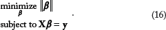
This achievement led to a large body of work on many aspects of the problem, proposing estimators for situations in which the covariance matrix of the normal population is known or unknown, extending this estimation procedure to non-normal populations, the Bayesian justification of the James–Stein estimator, and various attempts to improve upon the James–Stein estimator. Here, it is not possible to summarize the large amount of work done in this direction. We describe some of the key developments in the field, but for more information the readers are referred to other works.^24–28 The James–Stein estimator is given by ²³

$${\delta }_{Js}=\left(1-\frac{p-2}{{\Vert x\Vert }^2}\right)x.$$

(2)

It turns out that δ _JS is itself inadmissible and has a peculiar behavior for small values of |x|. In particular, the shrinkage factor $\left(1-\frac{p-2}{{\Vert x\Vert }^2}\right)$ becomes negative, in which case the sign of each component of the vector x changes. Baranchik proposed an improved estimator that dominates x.^21,29,30 This estimator is obtained by taking the “positive part” of the James–Stein estimator as

$${\delta }_{JS}^{+}={\left(1-\frac{p-2}{{\Vert x\Vert }^2}\right)}^{+}x,$$

(3)

where for a real number k, k⁺ = max(0,k). The estimator ${\delta }_{JS}^{+}$ has also an undesirable property that, when ${\Vert x\Vert }^2\le \frac{p-2}{n}$ , each element of the vector θ is estimated by zero. From the well-known results on smoothness of admissible estimators, ³¹ it follows that ${\delta }_{JS}^{+}$ itself is inadmissible. Baranchik ³⁰ widened the class of Stein's estimator by showing that any estimator of the form

$${\delta }_B=\left(1-\frac{\varphi \left(x\right)}{{\Vert x\Vert }^2}\right)x,$$

(4)

where φ(.) is (i) monotone, nondecreasing, and (ii) $0\le \varphi (\cdot )\le \frac{2\left(p-2\right)}{\left(n+2\right)}$ , dominates the usual estimator. Note that δ _JS is a special case of δ _B for φ(.) any constant satisfying (ii). Several other estimators have been proposed,^32,33 but Kubokawa's estimator ³⁴ is an estimator that dominates δ _JS and is admissible. A compelling intuition behind the James–Stein estimator and all previous extensions is as follows: Suppose an estimation of θ is desired and, rather than using the usual estimator x, we use an estimator ${\delta }_{\alpha }\triangleq \alpha x$ , where α is determined by minimizing the risk function. The risk of this estimator is given by

$$R\left(\theta ,{\delta }_{\alpha }\right)=E\left({\Vert \theta -{\delta }_{\alpha }\Vert }^2\right)={\Vert \left(1-\alpha \right)\theta \Vert }^2+p{\alpha }^2.$$

(5)

One can verify that the optimal choice of α that minimizes R(θ,δ_α) is given by

$${\alpha }_{opt}=1-\frac{p}{{\Vert \theta \Vert }^2+p},$$

(6)

which results in the minimum risk (the Bayes risk), given by

$$R\left(\theta ,{\delta }_{{\alpha }_{opt}}\right)=\frac{p{\Vert \theta \Vert }^2}{{\Vert \theta \Vert }^2+p}.$$

(7)

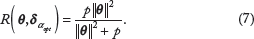
However, note that with the choice of α in (6), αx is not an estimator anymore because it depends on the unknown $\Vert \theta \Vert$ . However, since $E\left[{\Vert x\Vert }^2\right]={\Vert \theta \Vert }^2+p$ one can estimate ${\Vert \theta \Vert }^2+p$ in the denominator of (6) by ${\Vert x\Vert }^2$ and obtain the estimator $\left(1-p/{\Vert x\Vert }^2\right)x$ , which is in the form of the James–Stein estimator. An even better estimator is obtained if we replace p by p–2, which results in δ_JS.^23,24 Since the risk of the “usual estimator” δ _ML (x) is R(θ, δ _ML ) = p, we have

$$R\left(\theta ,{\delta }_{ML}\right)-R\left(\theta ,{\delta }_{{\alpha }_{opt}}\right)=\frac{p{\Vert \theta \Vert }^2}{{\Vert \theta \Vert }^2+p}.$$

(8)

It is evident that, when $\Vert \theta \Vert$ is large (compared to p), then $R\left(\theta ,{\delta }_{{\alpha }_{opt}}\right)\approx R\left(\theta ,{\delta }_{ML}\right)$ and we do not gain much by shrinking. However, for small values of $\Vert \theta \Vert ,R\left(\theta ,{\delta }_{{\alpha }_{opt}}\right)\approx 1<<p=R\left(\theta ,{\delta }_{ML}\right)$ . This shows that for a model (here the mean of a multivariate Gaussian distribution) that is sparse (contains many zero elements), the larger the dimension, the more we gain by shrinking.

Similar to the James–Stein estimation, ridge estimation is a type of shrinkage originally proposed in ³⁵ and developed further by many researchers. Consider the linear model

$$y=X\beta +\epsilon ,$$

(9)

where y is an n-dimensional observation vector, X is a known n × p matrix, β = [β₁, β₂,., β _p ]^T is a p-dimensional parameter vector to be estimated, and ∊ is an n-dimensional error vector with mean 0 and covariance matrix σ ² I _p . If we assume X is a full (column) rank matrix (p < n), the ordinary least-square solution to this familiar linear model is given by

$$\widehat{\beta }={\left(X^{T}X\right)}^{-1}{X}^{T}y.$$

(10)

However, when p > n, the solution (10) does not exist because X ^T X becomes degenerate. Even the solution obtained by generalized inverse form of matrix X ^T X does not work well. A possible solution was proposed by Hoerl and Kennard,^35–37 who replaced the residual sum of squares by its ℓ₂, penalized form, given by

$$L_2\left(\beta \right)\triangleq {\Vert y-X\beta \Vert }^2+\lambda {\Vert \beta \Vert }^2,$$

(11)

where λ > 0 denotes a penalty factor controlling the length of β. Minimizing L₂(β) results in the so-called ridge regression, given by

$$\widehat{\beta }={\left(X^{T}X+\lambda I_p\right)}^{-1}{X}^{T}y.$$

(12)

In this way, the inverse of possibly ill-conditioned X ^T X is stabilized by adding the scalar matrix λI _p . The value of λ is assumed to be a meta-parameter of the procedure and, in general, is estimated from a model-selection strategy such as cross-validation. ³⁸ A family of estimators closely related to the ridge estimator is obtained by considering the l₁ penalty factor in (11). In that case, the goal is to minimize

$$L_1\left(\beta \right)\triangleq {\Vert y-X\beta \Vert }^2+\lambda \Vert \beta \Vert .$$

(13)

Here, λ determines a trade-off between the approximation error $\left({\Vert y-X\beta \Vert }^2\right)$ and the sparsity of parameters $\Vert \beta \Vert$ . Of course, a more natural way for such a trade-off would have been the ℓ₀ penalty factor $\left({\Sigma }_{i=1}^p{1}_{\left\{{\beta }_i=0\right\}}\right)$ , but replacing ℓ₁ with ℓ₀ in (13) and trying to minimize the resulting risk function would be an NP-hard problem. ³⁹ The “least absolute shrinkage and selection operator” (lasso) technique proposed by Tibshirani ⁴⁰ is used to minimize L₁(β). Therein, Tibshirani formulates the following quadratic programming problem:

$$\begin{array}{c}\underset{\beta }{\text{minimize}}{\Vert y-X\beta \Vert }^2\\ \text{subject}\hspace{0.17em}\text{to}\Vert \beta \Vert \le t\end{array},$$

(14)

which is equivalent to minimizing L₁(β); to wit, for any λ in L₁(β);, there exists a t > 0 such that (14) has the same solution as minimizing L₁(β);. The key element in the popularity of the lasso is its ability to perform estimation and model selection at the same time. For a design matrix X such that X ^T X = I _p (orthonormal), understanding the mechanism of the lasso's model selection is straightforward. In this case, the lasso estimate of β_i, denoted by ${\widehat{\beta }}_i$ , is obtained by the soft shrinkage operator originally proposed by Donoho and Johnson ⁴¹ ; to wit, we have

$${\widehat{\beta }}_i-sign\left({\widehat{\beta }}_i^o\right){\left(\left|{\widehat{\beta }}_i^o\right|-\lambda \right)}^{+},$$

(15)

where ${\widehat{\beta }}_i^o$ is the solution of ordinary least-square and (x)⁺ = max(x,0). Evidently, for $\lambda >\left|{\widehat{\beta }}_i^o\right|,{\widehat{\beta }}_i$ is exactly zero. Therefore, in this case, having $\lambda >\left|{\widehat{\beta }}_i^o\right|,i=1,2,.,k,$ , is equivalent to choosing a subset of size k variables and setting all other parameters to 0. Therefore, for a large value of λ, many β _i values are set to 0 and the solution becomes sparse. For a general design matrix X, minimizing L₁(β); has no closed-form solution. Solving (14) using the algorithm proposed by Tibshirani ⁴⁰ is not efficient for large values of p, but efficient algorithms have emerged to compute the solution.^42–44 There has been a large body of work on generalizing the idea of the lasso, eg, elastic net, ⁴⁵ adaptive lasso, ⁴⁶ grouped lasso, ⁴⁷ fused lasso, ⁴⁸ and graphical lasso. ⁴⁹ The readers are referred to ⁵⁰ for a review of the various generalizations of the lasso technique. Before the emergence of the idea of the lasso, the idea of using ℓ₁ norm for sparse representation of signals was used in the signal processing community ⁴¹ (also see Appendix I in Ref. 39). Nevertheless, in signal processing, the idea was generalized and formalized later in Ref. 51, resulting in the basis pursuit (BP) framework. In signal processing applications, the BP is used to decompose a signal (y) into an optimal superposition of discrete dictionary waveforms (X) such as Fourier dictionary, wavelet dictionary, etc. The optimality is based on minimizing the ℓ₁ norm of coefficients (β) of the representation such that the solution becomes an affine subspace in Rp. Formally, BP solves

$$\begin{array}{l}\underset{\beta }{\text{minimize}}\Vert \beta \Vert \\ \text{subject}\hspace{0.17em}\text{to}\hspace{0.17em}X\beta =y.\end{array}$$

(16)

Therefore, by minimizing the ℓ₁ norm of coefficients, we are seeking for the sparsest possible solution. In the presence of noise, BP is used by solving a quadratically constrained linear program, which is a trade-off between a quadratic misfit and the ℓ₁ norm of coefficients ⁵¹ :

$$\begin{array}{l}\underset{\beta }{\text{minimize}}\Vert \beta \Vert \\ \text{subject}\hspace{0.17em}\text{to}\hspace{0.17em}{\Vert y-X\beta \Vert }^2\le \epsilon ,\end{array}$$

(17)

in which ∊ > 0 controls the amount of trade-off. As we have seen, the James–Stein estimation and ℓ₁ shrinkage (lasso-based or BP-based methods) are well suited to situations where the underlying model is sparse. Next, we review independent machinery for high-dimensional analysis in which the assumption of sparsity does not play a role.

Curse of Dimensionality and g-Analysis

Generalized consistent estimation (also known as Girko G-analysis) is a technique to construct estimators specific to situations in which the dimension is comparable to the number of samples. In this setting, an estimator is constructed such that it converges to the actual parameter in a “double-asymptotic” sense, to wit, in an asymptotic scenario in which dimension and sample size increase in a proportional manner, eg, n ↠ ∞, p ↠ ∞, and p/n ↠ c > 0. In this framework, the sparsity principle does not play a role. However, if the curse of dimensionality is intrinsic to frequentist statistics, then regardless of the model we use, there will still be a large gap between the complexity that we can capture through our model and the complexity of the phenomenon under study (if, of course, the phenomenon is complex per se). Therefore, in the subsequent discussion, we first examine the curse of dimensionality, its origin, and implications.

Curse of dimensionality

The curse of dimensionality, also known as the “peaking phenomenon” or the “Hughes phenomenon”, is generally considered as the known fact accounting for dimensionality reduction and feature selection.^6,52,53 Regarding the peaking phenomenon, McLachlan stated ⁵⁴ :

For training samples of finite size, the performance of a given discriminant rule in a frequentist framework does not keep on improving as the number p of feature variables is increased. Rather, its overall unconditional error rate will stop decreasing and start to increase asp is increased beyond a certain threshold, depending on the particular situation.

Jain and Waller stated ⁵² :

Thus, even if the cost of taking measurements is negligible, there exists an optimum measurement complexity, which is a function of the number of available training samples and the probability structure of the model.

Chandrasekaran and Jain pointed out:

It is known that, in general, the number of measurements in a pattern classification problem cannot be increased arbitrarily, when the class-conditional densities are not completely known and only a finite number of learning samples are available. Above a certain number of measurements, the performance starts deteriorating instead of improving steadily.

See Ref. 55 or p. 561 in Ref. 56 for more comments about this phenomenon. The first observation of peaking phenomenon is attributed to the work of Hughes. ⁵³ However, the peaking observed by Hughes was shocking to many scientists since it was contrary to the previously reported results on the lack of peaking for Bayes (optimal) classifiers. Hughes noted, “If insufficient sample data are available to estimate the pattern probabilities accurately, then a Bayes recognizer is not necessarily optimal”.^53,57 Various researchers correctly criticized Hughes’ work by pointing out that the paradoxial peaking phenomenon observed therein was not real and was due to the estimate of unknown cell probabilities from the data.^57–60 In other words, the peaking phenomenon observed by Hughes was essentially within a frequentist framework, not a Bayesian.

Nevertheless, it is now the general consensus that in the frequentist framework, the performance of a constructed classifier does not keep improving as more features are added. To be more precise, it is assumed that there is a certain point after which we should not keep adding features because the expected error rate of the classifier starts to increase (see above quotes as well as Refs. 6 and 56). Commonly, this certain point is referred to as the “optimal number of features”.^52,55 Nevertheless, all the aforementioned studies, and even terminologies such as curse of dimensionally or peaking phenomenon, give the impression that we should not learn from a large number of variables when a finite (and perhaps relatively small) number of samples is available.

Here, I shall try to convince you that the curse of dimensionally is not a phenomenon intrinsic to the frequentist framework. Instead, it is an artifact of many contemporary frequentist approaches. However, let us first review a few theoretical works that show peaking phenomenon in a frequentist setting.

In Ref. 6, the authors studied the peaking phenomenon in the context of discrete classification using a histogram rule. They considered multinomial distributions governing the data and characterized the expected error rate of the histogram rule over both sample space and a uniform prior distribution on the multinomial parameters. However, the complexity of the expression obtained there for the expected error rate did not let them achieve an analytical solution for the optimal dimension or analytical proof for the existence of a dimension at which the expected error rate is minimized.

Another work in this context is that of Jain and Waller, ⁵² who analytically studied the peaking phenomenon in connection with linear discriminant analysis (LDA) and in the context of Gaussian multivariate models. They used Bowker and Sitgreaves's^61,62 approximation of the expected error of LDA to determine an expression for the minimal increase in ${\delta }_p^2$ that justifies adding another feature (“avoid peaking”), where ${\delta }_p^2$ is the Mahalanobis distance given by

$${\delta }_p^2={\left({\theta }_1-{\theta }_0\right)}^T{\sum }^{-1}\left({\theta }_1-{\theta }_0\right),$$

(18)

where p denotes the dimensionality. They showed that the minimal increase in ${\delta }_p^2\left(\text{assuming}\hspace{0.17em}{\delta }_p^2>>\frac{4p}{n}\right)$ to keep the same expected error rate is given by

$${\delta }_{p+1}^2={\delta }_p^2=\frac{{\delta }_p^2}{n-3-p},$$

(19)

where n in the total number of samples in both classes. They also used this minimal increase expression to obtain various curves of expected error rate to show the peaking phenomenon. Nevertheless, their results were specific to LDA. Their observation should not be generalized to other models or even interpreted as a proof of omnipresence of peaking phenomenon in the frequentist framework (at least the way it is commonly presented). Moreover, the asymptotic expansion that Bowker and Sitgreaves used to develop their approximation of the expected error was essentially developed under the classical n ↠ ∞ and fixed p regime, which has a poor performance in a high-dimensional setting.

The salient point is that, even with the existing classifiers that have been developed through the classical statistical framework (n ↠ ∞, p fixed), the peaking phenomenon is not what is commonly perceived. To show this, in the following, we present an example in which even after the so-called optimal number of features has been found, we still keep adding features to the model. From earlier discussion, recall that the optimal number of features is generally considered as the number after which adding more features deteriorates the performance. However, in this example, we observe that after initial deterioration in the performance of the classifier, the performance again starts to improve after adding many features. Furthermore, we observe that even by considering all features in this example, the performance is still better than the performance at the so-called optimal point. Although these observations depend on the complexity of classifiers and the probabilistic structure of the problem, they demonstrate that learning from a large number of variables is plausible.

Consider a set of n = n₀ + n₁ independent and identically distributed (i.i.d.) training samples in Rp, where $x_1,x_2,.,x_{n_0}$ come from population ${\Pi }_0$ , and $x_{n_0+1},x_{n_0+2},\mathrm{\dots },x_{n_0+n_1}$ come from π₀ and ${\Pi }_1$ come from population π₁. The population π_i is assumed to follow a multivariate Gaussian distribution N(θ _i , σ), for i = 0,1, where θ _i and σ denote the mean and the covariance matrix, respectively. Consider the following discriminant function ⁶³ :

$$W\left({\overline{x}}_0,{\overline{x}}_1,x\right)={\left(x-\frac{{\overline{x}}_0+{\overline{x}}_1}{2}\right)}^T\left({\overline{x}}_0-{\overline{x}}_1\right),$$

(20)

where: ${\overline{x}}_0=\frac{1}{n_0}\sum _{i=1}^{n_0}{x}_i$ and ${\overline{x}}_1=\frac{1}{n_1}\sum _{i=n_0+1}^{n_0+n_1}{x}_i$ are the sample means for each class. The Euclidean-distance classifier (EDC) is given by

$$\psi \left(x\right)=\{\begin{array}{ccc}1,& \text{if}& W\left({\overline{x}}_0,{\overline{x}}_{1}x\right)\le 0\\ 0,& \text{if}& W\left({\overline{x}}_0,{\overline{x}}_{1}x\right)>0\end{array}.$$

(21)

That is, the sign of $W\left({\overline{x}}_0,{\overline{x}}_{1}x\right)$ determines the classification of the sample point x. The true error of ψ(x), denoted by ∊, is defined to be the probability of misclassification:

$${\epsilon }_{n,p}={\alpha }_0+{\epsilon }_0+{\alpha }_1{\epsilon }_1,$$

(22)

where α_i is the prior probability for class i and ∊_i is the error contributed by class i, which is given by

$${\epsilon }_i=P\left({\left(-1\right)}^{i}W\left({\overline{x}}_0,{\overline{x}}_1,x\right)\le 0|x\in {\Pi }_i,{\overline{x}}_0,{\overline{x}}_1\right).$$

(23)

From (23), we have

$${\epsilon }_i=\Phi \left(\frac{{\left(-1\right)}^{i+1}{\left({\theta }_i-\frac{{\overline{x}}_0+{\overline{x}}_1}{2}\right)}^T\left({\overline{x}}_0-{\overline{x}}_1\right)}{\sqrt{{\left({\overline{x}}_0-{\overline{x}}_1\right)}^T\sum \left({\overline{x}}_0-{\overline{x}}_1\right)}}\right).$$

(24)

Assuming n₀ = n₁ = n, α₀ = α₁ and σ = σ ² I _p , from the results of Raudys^64,65 (also see Refs. 66 and 67) we can approximate the expected error (over the sampling distribution) of EDC by

$$E\left[{\epsilon }_{n,p}\right]\approx \Phi \left(\frac{-{\delta }_p^2}{\sqrt{{\delta }_p^2+2J}}\right),$$

(25)

where ${\delta }_p^2$ is the Mahalanobis distance given by (18) and J = p/n. This formula is also credited to A.N. Kolmogorov (see p. 3 of Ref. 68). Raudys’ approximations of finite sample expectation of true error for LDA and its derivatives (including EDC) are based on the basic form of the double-asymptotic approach (n ↠ ∞, p ↠ ∞,p/n ↠ c). In Ref. 69, the authors compared Raudys’ approximation to several well-known approximations that have been obtained by classical approaches (n ↠ ∞, p fixed) and showed that the double-asymptotic approximations are significantly more accurate than classical approximations in analyzing the expected true error of LDA. In particular, even with n/p < 3, the double-asymptotic expansions yield excellent approximations that are far more accurate than others. ⁶⁹

Let b _(p) , denotes a column vector of size p with identical elements b. In order to examine the peaking phenomenon, we consider two 1700-dimensional Gaussian distributions where

$${\theta }_0={\theta }_1,{\theta }_0={\left[{0.2}_{\left(10\right)}^T,{0.05}_{\left(190\right)}^T,{0.03}_{\left(1200\right)}^T,0_{\left(300\right)}^T\right]}^T$$

with I _p being the identity matrix of size p. As described in Ref. 55, “best” features are generally added first and less useful features are added later. In our Gaussian model, the feature discriminative power is the same or reduces as we move to higher dimensions (see θ₀). Therefore, the first p features are our best features. At each p, we train a classifier on 100 p-dimensional observations taken from the two aforementioned Gaussian distributions. We determine the expected error rate of EDC from (25). Figure 1 shows E[∊ _n,p ] versus p in a logarithmic scale. The solid curve is obtained from (25). In order to ensure that this curve is not an artifact of using approximation (25), E[∊ _n,p ] has been estimated by Monte Carlo simulations for a few dimensions as follows:

Figure 1

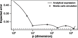
Expected error of Euclidean-distance classifier versus dimension for n₀ = n₁ = 100. The solid curve is obtained from theoretical results. The small circles are the result of simulation experiments for p = 10, 65, 200, 535, and 1,400.

The Monte Carlo simulation protocol.

• •

  Step I: Fix a of pair of p-dimensional Gaussian distribution π_o and π₁ with identity covariance matrices and means being the first p elements of vector θ₀ and θ₁ respectively. In simulations, we only consider p = 10, 65, 200, 535, and 1400.

• •

  Step II: From each distribution, generate a training set of size n = 100.

• •

  Step III: Using the training sample, construct EDC using (20) and (21).

• •

  Step IV: Find the true error of the constructed classifier using (22) and (24); this is possible because we have parameters of our model.

• •

  Step V: Repeat Steps II–-IV 500 times and take the average. The result is an estimate of E[∊ _n,p ].

The result of the Monte Carlo simulation for the five dimensions that we have considered is depicted by small circles in Figure 1: they align well with the theoretical results represented by the curve. As we see in this figure, as soon as we start adding more than 10 features to the EDC model, the performance starts deteriorating, but if we keep adding more and more features, at about p = 65, the performance again starts to improve. At p = 200, it has a local minimum and this behavior repeats one more time, resulting in a multi-hump curve. Interestingly, by considering all 1,700 features in the classifier, we obtain a performance better than the first local minimum at p = 10; to wit, E[∊_100,1700] = 0.273 < 0.276 = E[∊_100,10. Nevertheless, the best performance happens when p = 1,400 (E[∊_100,1400] = 0.254). Note that the EDC model is essentially a variant of the LDA classifier, which, under a Gaussian model, converges to the Bayes classifier as n ↠ ∞ and p fixed. It is natural to expect development of better classifiers from a mechanism such as the G-analysis framework, which is specifically designed for high-dimensional analysis. The conclusion to be drawn from this example is not to reject the peaking phenomenon – we can cite many examples that demonstrate that the peaking phenomenon is observed in the same way that is classically stated. Instead, this example demonstrates the following: 1) the way the curse of dimensionality is generally stated does not reflect what this phenomenon really is and may give a wrong impression to many practitioners, and 2) a compromise between complexity of the learning model and the number of predictors may achieve a better performance in a large-dimensional space than in a small one.

Double asymptotics and G-analysis

An example from random matrix theory

Random matrix theory (RMT) is a type of double-asymptotic analysis that is more focused on the analysis of spectral distribution of random matrices. The spectral distribution of random matrices is an important subject in multivariate analysis, as many statistics can be represented in terms of functionals of the spectral distribution of some matrices. ⁷⁰ Let {x_i,j, i,j = 1,2,…} be a double array of i.i.d. random variables with mean zero and variance 1. Let $x_j\triangleq {\left[x_{1,j},x_{2,j},.,x_{p,j}\right]}^T$ and define the data matrix X such that X = [x₁, x₂,., x_n]. The p × p sample covariance matrix is then defined by

$$C_{n,p}=\frac{1}{n-1}\sum _{l=1}^n\left(x_l-\overline{x}\right){\left(x_l-\overline{x}\right)}^T.$$

(26)

The empirical spectral distribution (ESD) of matrix C _n,p is given by

$$F_{C_{n,p}}(x)=\frac{1}{p}\sum _{i=1}^p{1}_{\left\{{\lambda }_i\left(C_{n,p}\right)\le x\right\},}$$

(27)

where λ_i(C _n,p ), i = 1,2,…,p are the eigenvalues of C _n,p and $1_{\{\cdot \}}$ is the indicator function. We consider two cases: 1) $x_{i,j}$ has a standard normal distribution; and 2) $x_{i,j}$ is taken from {–1,+1} with equal probability. A fundamental problem in high-dimensional analysis is to study the convergence of sequence of $F_{C_{n,p}}\left(x\right)$ The histograms in Figure 2A–C represent the empirical spectral distribution of one realization of matrix C _n,p for three cases in which p/n = 1/2 and, (a) p = 1,000 and n = 2,000; (b) p = 100 and n = 200; and (c) p = 20 and n = 40. Under a double-asymptotic regime where p ↠ ∞, n ↠ ∞, p/n ↠ c > 0, the empirical distribution converges almost surely to a nonrandom distribution function F_c with the density given by

$$f_c\left(x\right)={\left(1-1/c\right)}^{+}\delta \left(x\right)+\frac{1}{2\pi cx}\sqrt{{\left(x-x\right)}^{+}{\left(b-x\right)}^{+}},$$

(28)

where $a={\left(1-\sqrt{c}\right)}^2,b={\left(1-\sqrt{c}\right)}^2$ and δ(x) is the delta function. This result was obtained by Marčenko and Pastur in 1967 ⁷¹ and today is referred to as the M-P law. As we see in these histograms, for relatively large values of p and n [Figs. 2(A), (B)], there is a substantial agreement between the M-P law and the ESD of one realization of matrix C _n,p .

Figure 2

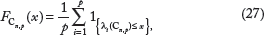
(A)–(C) Comparing the empirical spectral distribution of one realization of the covariance matrix with the limiting spectral distribution: (A) p = 1,000, n = 2,000; (B) p = 100, n = 200; (C) p = 20, n = 40. (D), (E) Comparing the average empirical spectral distribution of N realizations of the covariance matrix with the limiting spectral distribution: (D) p = 1,000, n = 2,000, and N = 10; (E) p = 100, n = 200, and N = 100; (F) p = 20, n = 40, and N = 10,000. Marčenko and Pastur ⁷¹ obtained the closed-form solution of the limiting spectral distribution by using the double-asymptotic framework.

Figure 2D–2F show the result of comparison between the average empirical spectral distribution of N realizations of covariance matrix C _n,p with the limiting spectral distribution in which N is 10, 100, and 10,000, for p = 1,000, 100, and 20, respectively (p/n = 1/2). As we see, there is a substantial agreement between the average empirical distribution and the M-P law in all three cases. Convergence of histograms in Figures 2A and 2D to the same limiting density presents an interesting property of the double-asymptotic regime; to wit, in this asymptotic regime the dependencies of the results on the realization of C _n,p disappear. Furthermore, the result is independent of the distribution of the elements in the double array: for both normal and binary random variables the limiting spectral distributions are identical.

The convergence of histograms in Figure 2(D)–(F) to the same density shows another interesting property of this operating regime: if we consider the average (expected) behavior of the ESD, the result of double asymptotics, although theoretically valid for p ↠ ∞ and n ↠ ∞, agrees well with the empirical result even for situations in which p and n are relatively small (Fig. 2F). Note that in many practical situations we are interested in average behavior of a statistic and, in this regard, double asymptotics can serve as a potential machinery for analyzing and synthesizing statistics. It is illuminating to compare the result of double-asymptotic analysis with the classical asymptotic analysis. The only information that we have from the classical asymptotic analysis is that, as n ↠ ∞ and for fixed p, the distribution of λ_i(C _n,p ) converges (almost surely) to a delta function at 1. Clearly, this information is completely useless in estimating the empirical spectral distribution in all cases considered in this example.

Emergence of double-asymptotic analysis

In the past few decades, double-asymptotic analysis, in general, and RMT, in particular, have found eminent roles in various disciplines, including nuclear physics, statistical mechanics, signal processing, wireless communications, biology, and economics.^70,72 Some scientists, such as Raj Nadakuditi, ⁷³ believe that RMT is “somehow buried deep in the heart of nature”. The first account of double-asymptotic analysis can be traced back to studying the limiting spectral distribution of random matrices of large dimension. This analysis was done by Eugene P. Wigner, the Nobel Prize winning physicist who, in the context of quantum physics and in connection with the energy levels of heavy nuclei, proved that the expected spectral distribution of Wigner matrices of increasing dimension converges to the semicircle law.^74–76 In quantum physics, any measurable physical quantity (a dynamical variable) of a system is represented by a self-adjoint operator (commonly referred to as the Hamiltonian) that acts in the state space. The Hamiltonian operator acting in state space can be represented in the matrix representation, resulting in matrix mechanics – which Heisenberg used to formulate quantum mechanics in the first place.^77,78 Concerning the rise of RMT in physics, Freeman Dyson writes ⁷⁹ :

By assuming all states of a very large ensemble to be equally probable, one obtains useful information about the overall behavior of a complex system, when the observation of the state of the system in all its detail is impossible. What is here required is a new kind of statistical mechanics, in which we renounce exact knowledge not of the state of a system but of the nature of the system itself. We picture a complex nucleus as a ‘black box’ in which a large number of particles are interacting according to unknown laws. The problem then is to define in a mathematically precise way an ensemble of systems in which all possible laws of interaction are equally probable.

And concerning the randomness of the Hamiltonian that appears in Schrödinger's equation, Mehta writes, ⁸⁰

In the case of the nucleus, however, there are two difficulties. First, we do not know the Hamiltonian and, second, even if we did, it would be far too complicated to attempt to solve the corresponding equation. Therefore, from the very beginning we shall be making statistical hypotheses on H [Hamiltonian], compatible with the general symmetry properties. Choosing a complete set of functions as a basis, we represent the Hamiltonian operators H as matrices. The elements of these matrices are random variables whose distributions are restricted only by the general symmetry properties we might impose on the ensemble of operators.

Here Mehta eloquently describes the reason why pioneers such as Wigner and Dyson associated the randomness of the Hamiltonian and, consequently, its corresponding matrix representation with the complexity of the nucleus (see Ref. 79 for more details). Beside the curse of dimensionality that we discussed earlier, the principle of parsimony is another motivation for an immediate use of dimensionality reduction regardless of the complexity of the phenomenon under study. While the principle of parsimony tells us that a simpler model is preferable to a competing complex model, it does not tell that all phenomena are simple. While the sparsity of parameters describing a phenomenon seems a tempting idea, not all phenomena are sparse. A heavy nucleus is a perfect example of a complex system. What Wigner did was not to create a parsimonious model to describe such a system. Instead, in his groundbreaking work, he increased the complexity of model to infinity by considering random matrices of infinite dimension.^74,75 As described in Ref. 81, the Bayesian philosophy dominated the statistics in the nineteenth century, but twentieth century was more a frequentist one. I believe that after the long 250-year-old debate between Bayesians and frequentists, if there is a revolution in statistical learning community (if not yet), it happens in shifting the low-dimensional analytical paradigm to a high-dimensional one (see the R.A. Fisher's quote in the introduction).

In the last 60 years, there have been an enormous number of studies in the context of random matrices of increasing dimension. The field has been developed to a large extent in the hands of F. J. Dyson,^79,82,83 M. L. Mehta,^84–87 L. A. Pastur,^71,88,89 V. L. Girko, J. W. Silverstein,^93–96 Z. D. Bai,^97–100 and Y. Q, Yin.^101–104 As estimated in Ref. 70, there has been more than 2,500 publications in the field from 1955 to 2004. The readers are encouraged to consult^70,72,80 for historical surveys of some of important results in the field.

A set of independent, but closely related work to previous studies, is the work of Raudys, Deev, Meshalkin, Serdobolskii, and Fujikoshi on the application of double asymptotics in classification.^105–112 This body of work is formalized as follows: consider a sequence of Gaussian discrimination problems with a sequence of parameters and sample sizes: $\left({\mu }_{p,0},{\mu }_{p,1},{\Sigma }_p,n_{p,0},n_{p,1}\right),p=1,2,\mathrm{\dots },$ where the means and the covariance matrix are arbitrary. Let us denote the limit under $n_0\to \infty ,n_1\to \infty ,p\to \infty ,\frac{p}{n_0}\to J_0<\infty$ , by $\underset{p\to \infty }{\lim }$ . In this setting, a large body of work has been devoted to characterizing the expected true error and estimated error of LDA and its variants. The readers are referred to the paper by Raudys and Young who conducted a review of articles in this context. ⁶⁵ It is commonly assumed that the Mahalanobis distance, ${\delta }_{\mu ,p}=\sqrt{{\left({\mu }_{p,0}-{\mu }_{p,1}\right)}^T{\Sigma }_p^{-1}\left({\mu }_{p,0}-{\mu }_{p,1}\right)}$ , is finite and $\underset{p\to \infty }{\lim }{\delta }_{\mu ,p}={\overline{\delta }}_{\mu }$ , where ${\overline{\delta }}_{\mu }$ denotes an arbitrary finite limiting point (see p. 4 of Refs. 67, 68, and 113). This condition ensures the existence of limits of performance metrics of relevant statistics.^67,68 The aforementioned asymptotics along with the limiting point conditions is also referred to as “Kolmogorov asymptotics”. ⁶⁸ Raudys's approximation of expected error rate of EDC that was presented in Ref. 25 is essentially based on the Kolmogorov asymptotics. As we discussed earlier, the result of the approximation of this type is far more accurate than its counterparts obtained from classical asymptotic settings (see Ref. 69 for a comparison). In the last two decades, the ideas of double asymptotics and, in particular, RMT have found eminent applications in engineering disciplines such as wireless communication. One of the first applications of this type of analysis in wireless communication was to characterize the performance of large multiuser linear receivers ¹¹⁴ and to study various properties of code division multiple access (CDMA) channels where the number of users and the length of spreading code is large.^115,116 These works paved the way for subsequent applications of RMT to study various properties of different communication channels; for instance, see Refs. 88, 117–120 to just cite a few articles.

G-analysis

Regarding the general statistical analysis of observation (G-analysis) and its connection to G-estimation and the Kolmogorov asymptotic conditions, V. L. Girko, one of the pioneers in developing this theory, writes:

The general statistical analysis of observations (G-analysis) is a mathematical theory studying some complex system S, such that the number m_n of parameters of its mathematical models can increase together with the growth of the number n of observations of the system S. The use of this theory consists in finding, with the help of observations of the system S, mathematical models (G-estimators) that approach the system S in some sense with a given rate under general assumptions on the observations: the existence of the distribution densities of the observed random vectors and matrices are not needed. The existence of several first moments of their components is all that is required; in addition, the numbers m_n and n satisfy the G-condition:

$${\overline{\lim }}_{n\to \infty }f\left(m_n,n\right)<\infty$$

(29)

where f(x,y) is some positive function increasing along x and decreasing along y. In most cases the function f(m_n, n) is equal to xy^–1. In this case the G-condition is also called the Kolmogorov condition.

The notation ${\overline{\lim }}_{n\to \infty }f\left(m_n,n\right)$ in the comment above denotes $\overline{\lim }\hspace{0.17em}{\sup }_{n\to \infty }f\left(m_n,n\right)$ . By taking f(m_n,n) = p/n, the framework boils down to the “usual” double-asymptotic setting in which p ↠ ∞, n ↠ ∞, p/n ↠ c. Using this machinery and throughout a decade, Girko developed about 50 estimators for various purposes. They are named as G₁-estimator (an estimator of generalized variance), G₂-estimator (an estimator of Stieltjes transform of the normalized spectral function), G₃-estimator (estimator of inverse covariance matrix), etc. Among them, we observe an estimator of the solution of the discrete Kolmogorov-Wiener filter (G₉), and an estimator of Anderson statistics (G₁₃). A summary of his results is presented in. ⁷ As pointed out by Gikro, an important property of G-analysis is that the result does not depend on the actual distribution of data. An example was given in the previous section in which the convergence of empirical spectral distribution to M–P law is independent of distribution of data (Fig. 2). This provides us with a mathematical machinery not only to calibrate many traditional estimators from the standpoint of double asymptotics (the so-called generalized consistency ³ ) but also to synthesize distribution-free techniques.

In recent years, several research groups, predominantly in signal processing community, have utilized the idea of G-analysis in various settings. For example, Mestre and Lagunas derived the generalized consistent estimator of the optimum loading factor in spatial filtering. ² In Ref. 3, Rubio and Mestre used the G-analysis to first evaluate the performance of a global minimum variance portfolio (GMVP) implementation based on shrinkage covariance matrix estimation and weighted sampling. Then they used the G-analysis to characterize the limiting expression of the realized variance and, based on that, they achieved a generalized consistent estimator of out-of-sample portfolio variance. ³ In Ref. 121, the authors developed an estimator of the optimal linear filter for both multiantenna array signals and financial asset returns. In Ref. 5, we utilized the G-analysis to calibrate a traditional estimator of the true error of the regularized LDA. This classical estimator, known as the plug-in estimator, is consistent under n ↠ ∞ and fixed p regime with a poor performance in small-sample situations. We observe that the calibrated new estimator can outperform not only the plug-in estimator but also other estimators of the true error, including Bootstrap 0.632 and cross-validation, in many situations in terms of bias and root-mean-square (RMS) error. Some other applications of G-analysis include estimating the eigenvalues and eigenvectors of sample covariance matrix ¹²² and estimating the direction of arrival (DoA) in linear sensor arrays. ¹²³

Extending G-analysis to Bayesian settings

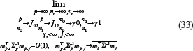
In Ref. 124, we characterized the moments of a Bayesian minimum mean-square error (MMSE) error estimator, ${\widehat{\epsilon }}^B{,}^{125,126}$ of the true error rate of LDA under a Gaussian model. There, we have characterized two sets of performance metrics: 1) the first, second, and cross moments of the estimated and actual errors conditioned on a fixed feature-label distribution, and 2) the unconditional moments. This means that we have obtained the metrics of performance ${\widehat{\epsilon }}^B$ depending on the evaluation scheme-conditional moments (unconditional moments) can be used as if the estimator is evaluated in a frequentist (Bayesian) framework. We set up a series of conditions to which we refer as the Bayesian–Kolmogorov asymptotic conditions. These conditions allow us to characterize the performance metrics of Bayesian MMSE error estimation in an asymptotic sense. The Bayesian–Kolmogorov asymptotic conditions are set up based on the assumption of increasing n, p, and the certainty parameter v, with an arbitrary constant limiting ratio between n and p, and n and v. To our knowledge, these conditions permit, for the first time, the application of G-analysis in a Bayesian setting. To analyze the Bayesian MMSE error estimator ${\widehat{\epsilon }}_i^B$ , we consider a sequence of Gaussian discrimination problems as

$$\left({\mu }_{p,0},{\mu }_{p,1},{\Sigma }_p,n_{p,0},m_{p,0},m_{p,1},{\upsilon }_{p,0},{\upsilon }_{p,1}\right),p-1,2,\dots ,$$

(30)

where σ and μ _i are the covariance matrix (assumed to be known) and the mean of Gaussian feature label distributions, respectively, and σ/v_i and m. are the covariance matrix and the mean of the Gaussian prior distribution on μ _i . We assume that the following limits exist for $ij=0,1:\underset{p\to \infty }{\lim }{m}_{p,i}^T{\Sigma }_p^{-1}{\mu }_{p,j}=\overline{m_i^T{\Sigma }^{-1}{\mu }_j,}\underset{p\to \infty }{\lim }{m}_{p,i}^T{\Sigma }_p^{-1}{m}_{p,j}=\overline{m_i^T{\Sigma }^{-1}{m}_j,}$ and $\underset{p\to \infty }{\lim }{\mu }_{p,i}^T{\Sigma }_p^{-1}{\mu }_{p,j}=\overline{{\mu }_i^T{\Sigma }^{-1}{\mu }_j,}$ where $\overline{m_i^T{\Sigma }^{-1}{\mu }_j},\overline{m_i^T{\Sigma }^{-1}{m}_j}$ and $\overline{{\mu }_i^T{\Sigma }^{-1}{\mu }_j}$ are some constants to which the limits converge. These are generalizations of $\underset{p\to \infty }{\lim }{\delta }_{\mu ,p}={\overline{\delta }}_{\mu }$ condition that was previously stated in the Kolmogorov asymptotics context. All of the aforementioned conditions along with ${\upsilon }_i\to \infty ,\frac{{\upsilon }_i}{n_i}\to {\gamma }_i<\infty$ , construct the Bayesian–Kolmogorov asymptotic conditions. To summarize, the asymptotic regime that we considered there is characterized by the following limit:

$$\begin{array}{c}\underset{p\to \infty ,n_i\to \infty ,{\upsilon }_i\to \infty }{\lim }\\ \underset{n_0}{\overset{p}{\to }}{J}_0,\underset{n_1}{\overset{p}{\to }}{J}_1,\underset{n_0}{\overset{{\upsilon }_0}{\to }}{\gamma }_0,\underset{n_0}{\overset{{\upsilon }_0}{\to }}{\gamma }_1\\ {\gamma }_i<\infty ,\hspace{0.17em}{J}_i<\infty \\ \begin{array}{cc}{m}_{p,i}^T{\Sigma }_p^{-1}{\mu }_{p,j}=O\left(1\right),& m_{p,i}^T{\Sigma }_p^{-1}{\mu }_{p,j}\to \overline{m_1^T{\Sigma }^{-1}{\mu }_j}\\ m_{p,i}^T{\Sigma }_p^{-1}{m}_{p,j}=O\left(1\right),& m_{p,i}^T{\Sigma }_p^{-1}{m}_{p,j}\to \overline{m_1^T{\Sigma }^{-1}{m}_j}\\ m_{p,i}^T{\Sigma }_p^{-1}{\mu }_{p,j}=O\left(1\right),& {\mu }_{p,i}^T{\Sigma }_p^{-1}{\mu }_{p,j}\to \overline{{\mu }_1^T{\Sigma }^{-1}{\mu }_j}\end{array}\end{array}$$

(31)

This limit is defined for a situation in which there is a conditioning on a specific value of feature label distribution parameters such as μ _p,i . Therefore, in this case μ _p,i is not a random variable, and for each p, it is a vector of constants. Absent such conditioning, the sequence of discrimination problems and the above limit reduce to

$$\left({\Sigma }_p,n_{p,0},n_{p,1},m_{p,0},m_{p,1},{\upsilon }_{p,0},{\upsilon }_{p,1}\right),\hspace{0.17em}p=1,2,\dots ,$$

(32)

and

$$\begin{array}{c}\underset{p\to \infty ,n_i\to \infty ,{\upsilon }_i\to \infty }{\lim }\\ \underset{n_0}{\overset{p}{\to }}{J}_0,\underset{n_1}{\overset{p}{\to }}{J}_1,\underset{n_0}{\overset{{\upsilon }_0}{\to }}{\gamma }_0,\underset{n_1}{\overset{{\upsilon }_1}{\to }}{\gamma }_1\\ {\gamma }_i<\infty ,\hspace{0.17em}{J}_i<\infty \\ \begin{array}{cc}{m}_{p,i}^T{\Sigma }_p^{-1}{m}_{p,j}=O\left(1\right),& m_{p,i}^T{\Sigma }_p^{-1}{m}_{p,j}\to \overline{m_1^T{\Sigma }^{-1}{m}_j}\\ & \\ & \end{array}\end{array}$$

(33)

respectively The accuracy of the closed-form expressions derived in this work is remarkable. We believe this framework can serve as a potential technique in the future to calibrate various Bayesian estimators from a frequentist point of view: to wit, to optimize the performance of a developed Bayesian method for a specific parametric distribution with unknown parameters.

Discussion

In recent years, various statistical learning rules have been put forward for cancer diagnosis, prognosis, discriminating stages of cancer, types of pathology, and duration of survivability based on molecular profiles such as gene or protein expression patterns and single nucleotide polymorphism genotypes. Such a biomarker discovery process in high-throughput genomic and proteomic profiles has presented the statistical learning community with a challenging problem, namely how to learn from a large number of variables and a relatively small sample size. The properties of high-dimensional data, though, are not well understood. ¹²⁷ A high-dimensional setting is not the place to rely on intuition, nonrigorous propositions, and heuristics. At the same time, the classical notion of statistical consistency, which guarantees the performance of many classical statistical techniques, falters because this notion guarantees the performance of a technique in situations where the number of measurements unboundedly increases (n ↠ ∞) for a fixed dimensionality of observations, p. In a finite sample operating regime, this implies that in order to expect an acceptable performance from a statistical technique, we need to have many more sample points than variables – a scenario opposite to what we currently face in high-throughput biology. Despite many achievements in the last few decades in the field of statistical learning, some of the most elementary problems remain unsolved. In this regard, Serdobolskii stated ⁶⁸ :

It is difficult to describe the recent state of affairs in applied multivariate methods as satisfactory. Unimprovable (dominating) statistical procedures are still unknown except for a few specific cases. The simplest problem of estimating the mean vector with minimum quadratic risk is unsolved, even for normal distributions. Commonly used standard linear multivariate procedures based on the inversion of sample covariance matrices can lead to unstable results or provide no solution in dependence of data. Thus nearly all conventional linear methods of multivariate statistics prove to be unreliable or even not applicable to high-dimensional data.

Two mathematical-statistical machineries, discussed herein, show promising results in constructing techniques of high-dimensional data analysis: 1) shrinkage, and 2) Girko G-analysis. This paper presented a brief history of development, the underlying assumptions, and some of important results of each machinery. While in the last decade there has been some effort to create statistical software packages from some of the shrinkage methods, the methods developed through G-analysis remain mostly in the literature and unknown to many theoreticians and practitioners. Some effort from applied statistics and the signal processing community seems worthwhile in order to create ready-to-use software packages from these methods. In addition, practical implications of the underlying assumptions in G-analysis need further investigation. For example, we assumed n ↠ infin;, p ↠ infin;, p/n ↠ c, 0 c < ∞ along with some conditions on the existence of moments of random variables involved. In an asymptotic sense, the results are applicable to any ratio of p/n. However, in a finite-sample regime, it would be interesting to study the robustness of designed methods with respect to this ratio. Other natural directions that deserve further research in this line of work are 1) understanding the true nature of the so-called curse of dimensionality phenomenon, 2) the connection between G-analysis conditions and the curse of dimensionality, 3) the possibility of using G-analysis in creating lasso-like operators that have the capability of performing model selection, and 4) extending G-analysis to Bayesian statistics.

Author Contributions

Conceived the concepts: AZ. Wrote the first draft of the manuscript: AZ. Developed the structure and arguments for the paper: AZ. Made critical revisions: AZ. The author reviewed and approved of the final manuscript.