Sage Journals: Discover world-class research

Abstract

Ovarian cancer is the fifth leading cause of death among female cancers. Front-line therapy for ovarian cancer is platinum-based chemotherapy. However, the response of patients is highly nonuniform. The TCGA database of serous ovarian carcinomas shows that ~10% of patients respond poorly to platinum-based chemotherapy, with tumors relapsing in seven months or less. Another 10% or so enjoy disease-free survival of three years or more. The objective of the present research is to identify a small number of highly predictive biomarkers that can distinguish between the two extreme responders and then extrapolate to all patients. This is achieved using the lone star algorithm that is specifically developed for biological applications. Using this algorithm, we are able to identify biomarker panels of 25 genes (of 12,000 genes) that can be used to classify patients into one of the three groups: super responders, medium responders, and nonresponders. We are also able to determine a discriminant function that can divide the entire patient population into two classes, such that one group has a clear survival advantage over the other. These biomarkers are developed using the TCGA Agilent platform data and cross-validated on the TCGA Affymetrix platform data, as well as entirely independent data from Tothill et al. The P-values on the training data are extremely small, sometimes below machine zero, while the P-values on cross-validation are well below the widely accepted threshold of 0.05.

Keywords

ovarian cancer platinum chemotherapy prediction of patient response

Introduction

Background

Ovarian cancer is the fifth most deadly form of cancer for females, after lung, breast, colon, and pancreatic cancers. It is estimated that in the United States during 2015, there will be 21,290 new cases of ovarian cancer and 14,180 deaths.¹ Standard front-line therapy for ovarian cancer consists of some form of taxane (paclitaxel) coupled with some form of platinum (cisplatin or carboplatin), hereafter referred to as platinum-based chemotherapy. Patient response to front-line therapy is not uniform. Because it is not possible to monitor a patient continually to assess response to therapy, one can use progression-free survival (PFS) or overall survival (OS) as somewhat imperfect proxies for patient response. Initially, 70%–80% of patients appear to respond to front-line therapy.² However, based on the TCGA database of serous ovarian carcinoma,³ ~10% of patients have PFS of seven months or less. In contrast, ~10% of patients enjoy PFS of three years or more and the rest most ultimately relapse and die of disease progression.⁴

Therefore, it is imperative to be able to predict the responsiveness of ovarian cancer patients to front-line therapy. Our premise is that if there is a set of genetic biomarkers that are indicative of patient response, their influence is likely to be more pronounced at the two extreme ends of patient response. Therefore, if we succeed in developing one or more classifiers that are capable of discriminating between these two extreme cases, then these classifiers can be extended to encompass the entire patient population, which is precisely the objective of the present paper. We develop four different classifiers based on the TCGA Agilent data set and then validate them on the TCGA Affymetrix data set, as well as an independent data set from Tothill et al.⁵

Current status

At the moment, CA125 is the only known biomarker to assess the effectiveness of therapy in ovarian cancer. However, CA125 levels are primarily used as a post facto measure that determines whether therapy is working and not as a predictive indicator of whether platinum chemotherapy is likely to work. Moreover, CA125 by itself is not deemed to be sufficient as an indicator. In a recent review, it is emphasized that germline mutations in BRCA1 and BRCA2 lead to enhanced lifetime risk of developing ovarian cancer, as well as in lowering the age of initial onset of the disease.⁶ Over the years, several papers have proposed various sets of biomarkers. A recent paper² states that “There were 139 studies that reported an association between biomarker expression and overall survival (OS) with univariate analysis, whereas with multivariate analysis, an association between biomarker expression and OS was reported in 47 studies.” and “The number of studies that evaluated an association between biomarker expression and progression-free survival (PFS) with univariate analysis and multivariate analysis was 66 and 20 studies, respectively.” Unless one goes through each of these studies individually, one would not know whether the analysis also incorporated additional factors, such as age, weight, number of pregnancies, stage of disease, and size of tumor.

In general, most of the papers fall into one of the two categories. In the first category, the authors have a candidate biomarker in mind. The available patient pool is divided into two groups, and the mean values of the candidate biomarker across each group are computed. If there is a statistically significant difference between these mean values (using the Student's t-test for example), then the candidate biomarker can be said to have passed one filter for utility. Biomarkers that are identified using this approach include the protein TR3 and its associated gene NR4A1,⁷ Tau protein and its associated gene MAPT,⁸ and β-tubulin and its associated gene TUBB.^9,10 In such studies, it is implicitly assumed that only the putative biomarker being studied exhibits a significant variation across groups, while “all other things are equal.” However, in the TCGA Agilent mRNA data set,³ there are more than 200 genes that show a statistically significant difference in mean values between the two extreme cohorts (super responders [SRs] and nonresponders [NRs]). Thus, examining a few genes (or other biomarkers) in isolation may lead to incorrect conclusions.

The second approach is to apply some kind of machine learning algorithms to the data at hand, thereby obtaining a panel of biomarkers. Examples of such approaches include Ref. 11, in which 322 samples were analyzed to generate a 349-gene biomarker panel that performs very well, but when the 349 genes are reduced to 18 genes, the performance on the test data is poor,¹² in which a 300-gene Ovarian Carcinoma Index is constructed on the basis of 80 samples, which is then tested on 118 samples; and in Ref. 4, a panel of 14 genes is identified to differentiate between early relapse and late-stage relapse. It is worth pointing out that all of the abovementioned papers use some variant of the support vector machine (SVM) to find the biomarkers. Indeed, this is reasonable, as the SVM is very robust and is widely used in many application areas.

An excellent review of several studies can be found in Ref. 13. In Ref. 14, the authors started with a set of 151 DNA repair genes and identified a subset of 23 such genes that are then used to construct a score. Within the family of DNA repair genes, it has been suggested that various genes that arise in the nucleotide excision repair and base excision repair pathways, and single-nucleotide polymorphisms in these genes, have a role to play,¹⁵ for example, ERCC and XRCC families of genes. Finally, a BRCA2 mutation is associated with improved survival and improved chemotherapy response,¹⁶ although mutations in BRCA1 or BRCA2 are associated with enhanced risk and earlier onset of ovarian cancer.⁶ A possible explanation is that responsiveness to PARP-based therapy is enhanced with BRCA mutations. A recent paper that made an extensive and thorough benchmark study concluded that no ovarian cancer gene expression signature is ready for clinical use yet.¹⁷ In summary, there is no shortage of claimed biomarkers. However, none of these papers contains a molecular signature, that is, a procedure for converting measured values of the biomarkers (usually gene expression levels) into a numerical score. The development of such a signature and not just a biomarker panel is one of the motivations behind the present paper.

Contributions of the paper

In the present paper, we analyze the TCGA ovarian cancer data that consists of molecular measurements and clinical outcomes on nearly 600 serous carcinomas. We study gene expression levels as molecular measurements and PFS and OS as clinical parameters. Patients whose clinical parameters (survival, OS or PFS) are at the two extremes are identified using the user-defined thresholds, as described subsequently. Then, we apply an algorithm named “lone star” developed within our research group to extract biomarkers and an associated molecular signature that can discriminate between extreme patients with respect to these clinical parameters. Then, this molecular signature is extended to the entire patient population in the TCGA study. In this manner, we are able to develop a three-way classification procedure for assigning each patient into one of the three categories, namely, SR, medium responder (MR), and NR. We also use the discriminant function developed for the extreme responders to divide the entire patient population into two groups, namely, those with a positive score and those with a negative score. Kaplan–Meier curves are plotted for these two groups, and it is shown that the patients with positive score exhibit a clear survival advantage compared to those with a negative score.

The lone star algorithm was initially presented in Ref. 18 and is described in detail in Ref. 19. A brief description of the algorithm is given in the Approach and methods section. The source code of an MATLAB implementation of the lone star algorithm is freely available at the following URL: http://sourceforge.net/projects/lonestar/

Therefore, the algorithm can be readily used by even those unfamiliar with machine learning theory, without having to get into its inner workings. The biomarker panels developed on the TCGA data are then validated on an independent data set due to Ref. 5.

Approach and Methods

General approach

The broad approach adopted in this paper is now described. The TCGA Agilent data set consisting of molecular measurements on roughly 600 serous ovarian carcinomas³ is chosen as the training data set, while the corresponding TCGA Affymetrix data set³ and the Tothill data set⁵ are chosen for validating the predictions. Of note, the validation data sets also consist solely of serous carcinomas. The TCGA Affymetrix data set serves to establish that our method is portable across platforms, while the Tothill data set serves to establish that our method is portable across both platforms and data sets. Given the training data set, a number X between 0 and 50 is chosen. The top X percentile in terms of patient response is defined to be SRs and the bottom X percentile is defined to be NRs. Those in the middle are defined to be MRs. Of note, the best responders should be called SR and the worst responders should be called NR, while those in-between should be called MR. The precise percentile cut-off, referred to as X earlier, is to some extent arbitrary. We have carried out the exercise below for the values of X ranging from 10 percentile to 50 percentile (that is, no MR category). The choice X = 33, thus dividing the patients into three equal-sized groups, works best, although the results for other choices of X are not much different and are available from the authors. Once the three categories of patients are defined, a recently proposed algorithm,^18,19 known as lone star, is applied to the training data, after the initially large number of features (genes) is pruned by some prefiltering. This step results in the definition of a discriminant function that is a linear combination of the expression values of the reduced feature set. The value of this discriminant function is computed for all patients, based on which patients are assigned to three groups: SR, MR, and NR. This results in a 3 × 3 contingency table (actual versus predicted group) and P-value is computed. In the next step, the patients are divided into two classes, namely, those with positive discriminant values and those with negative discriminant values. In principle, if our prediction methodology is any good, the positive class should have a survival advantage over the negative class. Kaplan–Meier curves are plotted for the two groups, and the P-value of the results obtained is computed for each case.

Definition of patient response

Patient response can be measured in two different ways, namely, OS and PFS. Though these two are broadly correlated, the correlation is by no means perfect. For instance, OS is determined not just by the efficacy of the therapy but also by other factors, such as age and general health. PFS is also subjective because the date on which a tumor is recorded as having progressed is the day on which it is observed to have progressed, whereas in reality the progression would have taken place at some unknown date between that observed date and the date of the previous checkup. Thus, the disparity between the recorded date of progression and the actual date of recurrence could be several months. It was not a priori clear which clinical parameter would lead to better predictions. Therefore, predictors were developed based on each parameter, and their performance was compared. Similarly, during the validation step too, the survival advantage of the group Δ₊ (those with positive discriminant values) against the group Δ_– (those with negative discriminant values) can be computed using either OS or PFS as the clinical parameter.

Definition of extreme responders

As stated earlier, patients whose survival is within the top X percentile are called SRs, while those in the bottom X percentile are called NRs. This raises the question, what value of X should be chosen? Very small values of X would cause almost all patients to be labeled as MRs, while an overly large value of X would cause almost no one to be classified as an MR. Various values of X from 10 to 50 were tried. The best results were obtained with X = 33%, meaning that the top one-third, middle one-third, and bottom one-third were labeled as SR, MR, and NR, respectively. Therefore, only those results are reported, though the results for other choices of X are available upon request.

In the TCGA database, there are 565 serous carcinoma samples for which information is available on days-to-death, days-to-recurrence, and/or days-to-last follow-up. If PFS is used as the criterion, the patients with PFS ≤283 days were classified as NRs, while patients with PFS ≥574 days were classified as SRs. If OS is used as the criterion, then patients with OS ≤504 days were classified as NR, while those with OS ≥1202 days were classified as SR. Of note, in both the TCGA Agilent and TCGA Affymetrix databases, these break points produced 189 NRs, 188 MRs, and 188 SRs. Of note, the demographic features of the three classes were quite similar. This can be ascertained from the TCGA data set. However, when the classifier was applied to the Tothill data set, the labels of NR, MR, and SR were determined solely on the basis of the survival times, both OS and PFS. Consequently, the fraction of the NR, MR, and SR samples does not necessarily correspond to the 33rd percentile.

Prefiltering the feature set

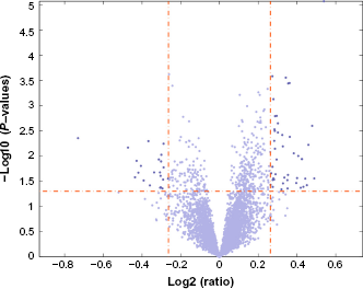
There are roughly 12,000 genes for which measurements are available in all three data sets (TCGA Agilent, TCGA Affymetrix, and Tothill). While developing the classifier for the training data, it is not desirable to run the lone star algorithm using all 12,000+ genes. Some prefiltering is desirable based on the combination of two attributes: (i) the t-test statistic that compares the mean values of a gene over the two groups and (ii) the fold change of the mean values over each group. Figure 1 illustrates the prefiltering method used. The prefiltering can either be loose, resulting in a large number of initial features that are then reduced further via the lone star algorithm, or be tight, meaning that the initial feature set passed on to the lone star algorithm is rather small.

Figure 1

Volcano plot of the negative logarithm of the t-test scores on the vertical axis and the fold changes on the horizontal axis.

The tight prefiltering used the following parameters: fold change of at least 1.25 between the averages of a gene's expression level over the two classes and the P-value of at most 0.05 between the average expression levels of the two classes, as computed using the t-test. This resulted in the retention of just 67 of roughly 12,000 genes for OS and 59 of roughly 12,000 genes for PFS. The loose prefiltering used the following parameters: fold change of at least 1.175 and the P-value of at most 0.1. This resulted in 208 genes selected for the OS and 181 genes selected for PFS.

The above discussion can be summarized in Table 1. There are four different combinations that are assessed in this paper: OS or PFS as clinical parameters and tight or loose prefiltering.

Table 1

The four classifiers studied in this paper.

CLASSIFIER NO.	CLINICAL PARAMETER	PRE-FILTERING
Classifier No. 1	Overall survival	Tight
Classifier No. 2	Overall survival	Loose
Classifier No. 3	Progression-free survival	Tight
Classifier No. 4	Progression-free survival	Loose

Lone star algorithm

For each of the four situations described in Table 1, the lone star algorithm was used to develop a binary classifier to identify a handful of highly predictive features, together with an associated linear discriminant function, that could be used to distinguish between the two sets of extreme responders. The following discussion is essentially reproduced from Ref. 19 in order to make the present paper self-contained.

The lone star algorithm is a very versatile and general-purpose algorithm developed in Ref. 18 and elaborated in Ref. 19, for the purpose of identifying a small number of highly predictive features from tens of thousands of measured features. It combines various ideas in machine learning, such as the l₁-norm SVM,²⁰ recursive feature elimination (RFE),²¹ and stability selection.²² The SVM formulation presupposes that every feature has an equal dynamic range. Therefore, for each feature, the vectors measured across all samples are converted into Z-scores by subtracting the mean and dividing by the standard deviation.

In case, we are given a set of labeled data here xⁱ ∊ Rⁿ and y_i ∊ {–1,1} for i = 1, 2, …, m. Therefore, n denotes the number of features and m denotes the number of samples. The feature vector xⁱ is viewed as a row vector. The objective is to choose a subset of features F ⊆ {1, …, n}, a weight vector w ∊ Rⁿ, and a threshold θ ∊ R, such that (a) the discriminant function f(x_i) = x_iw – θ has the same sign as y_i for most indices i, (b) w_j = 0 for all j ∉ F, and (c) |F|« m.

In other words, the discriminant function f is linear and the set of features used by the discriminant has smaller cardinality than the number of samples. Define

P = {i : y_{i} = 1} a n d N = {i \in y_{i} = - 1}

and let m₁ = |P| and m₂ = |N|. The algorithm consists of an iterative loop and a final classifier generation step. Steps 1–3 comprise the iterative loop, and step 4 is the final classifier generation.

Set the iteration counter to 1, the feature set F to the set of significant features, the feature count s₁ to |F|, and the iteration count i to 1, and then proceed to the iterative loop.

Stability selection: fix an integer l. Choose k₁ from the m₁ positive samples and k₂ from the m₂ negative samples at random as the training set of samples. Repeat this random choice l times, so that there are l different pairs of training samples: k₁ from the class P and k₂ from the class N. Ensure that k₁ and k₂ are roughly equal and lesser than m₁/2 and m₂/2, respectively.

l₁-Norm SVM: for each pair of k₁ and k₂ training samples, solve the following l₁-norm SVM formulated in Ref. 20:

\min_{w, θ, y, z} (1 - λ) [α \sum_{j = 1}^{k_{1}} y_{j} + (1 - α) \sum_{j = 1}^{k_{2}} z_{j}]

subject to the constraints

\begin{matrix} w^{t} x_{j} - θ + y_{j} \geq 1, j \in P, w^{t} x_{j} - θ - z_{j} \leq - 1, j \in N, \\ y \geq 0_{k_{1}}, z \geq 0_{k_{2}} . \end{matrix}

The parameter λ should be chosen close to zero, but not exactly zero. The parameter α should be chosen as 0.5 if sensitivity and specificity are equally important. The parameter α should be chosen to be <0.5 to place more emphasis on sensitivity, whereas α should be chosen to be >0.5 to place more emphasis on specificity.

RFE: The previous step results in l different optimal weight vectors, $w_{1}^{i}, \dots, w_{l}^{i}$ , where i is the iteration count. Each weight vector will have a different number of non-zero components. Compute the average number of nonzero components, round upward to the next integer, and denote this integer as rⁱ. Compute the average of all l weight vectors. Retain the rⁱ components with the largest magnitude and discard the rest. Increase the iteration counter i, set s^{i + 1} = rⁱ, and proceed to step 3. If Rⁱ = sⁱ, meaning that no features can be discarded, the iterative step is complete; hence, proceed to the next step.

Final classifier generation: When this step is reached, the set of features is finalized. Run the l₁-norm SVM on l different randomly chosen pairs of (k₁, k₂) training samples to generate l different classifiers and evaluate the performance of each of the l classifiers on the remaining (m₁ – k₁ m₂ – k₂) samples. Determine the accuracy, sensitivity, and specificity of each of the l classifiers. Average the weights and thresholds of the best-performing classifiers to generate an overall classifier.

Results

Development of binary classifiers

The lone star algorithm was applied to each of the four situations, as described in Table 1. In this subsection, the details of the resulting classifiers and their performance on the training data set, namely, TCGA Agilent, are given.

For PFS, with tight filtering and 59 genes as the starting point, the algorithm resulted in 25 genes being chosen as the most predictive features. For OS, 67 genes as the starting point resulted in 28 genes being chosen. The exercise was then repeated using a less aggressive or loose prefiltering step, so that the lone star algorithm has a larger number of initial features to choose. When OS was used as the criterion, the initial feature set consisted of 208 genes, of which 26 were finally chosen. When PFS was used as the criterion, the initial feature set consisted of 181 genes, of which 26 were finally chosen. Of note, though the number of finally selected features was comparable for all the four classifiers, the actual features themselves were different. Table 2 lists the finally selected features in the two classifiers based on OS with tight and loose prefiltering, while Table 3 lists the finally selected features in the two classifiers based on PFS with tight and loose prefiltering. In each case, the expression values of all genes are converted into Z-scores by subtracting the mean and dividing by the standard deviation across all SR + NR samples. The Z-score of each gene is multiplied by the weight shown, and the resulting weighted sum is compared to the bias term. If the weighted sum exceeds the bias, the sample is assigned to the positive (SR) class, whereas if the weighted sum is smaller than the bias, the sample is assigned to the negative (NR) class.

Table 2

Classifier nos. 1 and 2 – classifiers for OS.

ENTREZ GENE ID	GENE SYMBOL	WEIGHT	ENTREZ GENE ID	GENE SYMBOL	WEIGHT
241	ALOX5AP	–0.5630	953	ENTPD1	–0.7066
3764	kcnj8	–0.4870	54704	Pdp1	–0.6358
26290	GALNT8	–0.4393	1410	CRYAB	–0.5821
25790	Ccdc19	–0.3118	3764	kcnj8	–0.4942
2857	GPR34	–0.3116	5266	PI3	–0.4846
8483	CILP	–0.3039	25790	Ccdc19	–0.4362
794	CALB2	–0.2889	6236	RRAD	–0.4067
55016	MARCH1	–0.2662	10218	angptl7	–0.3554
6356	Ccl11	–0.2458	26290	GALNT8	–0.3522
64231	MS4A6A	0.1312	9033	pkd2H	–0.3252
25924	MYRIP	0.2086	10753	Capn9	0.2204
962	Cd48	0.2207	728621	CCDC30	0.2306
10753	Capn9	0.2422	57612	KIAA1466	0.2680
51284	TLR7	0.2827	3918	LAMC2	0.3141
1634	DCN	0.2845	404093	CUEDC1	0.3931
123872	LRRC50	0.2881	4147	Matn2	0.3981
79623	Galnt14	0.2937	1674	DES	0.4020
26585	GREM1	0.3075	203102	ADAM32	0.4241
5016	Ovgp1	0.3079	5521	PPP2R2B	0.4337
5276	serpini2	0.3439	9450	LY86	0.4763
6387	CXCL12	0.3519	8470	SORBS2	0.4815
56143	PCDHA5	0.3777	135138	Pacrg	0.5750
135138	Pacrg	0.3992	7130	TNFAIP6	0.5876
4147	Matn2	0.4722	1118	CHIT1	0.6102
1118	CHIT1	0.4867	1360	Cpb1	0.6115
			23144	ZC3H3	0.7026
	Bias	0.0150		Bias	0.0924

Table 3

Classifier nos. 3 and 4 – classifiers for PFS.

ENTREZ GENE ID	GENE SYMBOL	WEIGHT	ENTREZ GENE ID	GENE SYMBOL	WEIGHT
26290	GALNT8	–0.3878	3696	ITGB8	–0.5790
79908	BTNL8	–0.3711	1301	COL11A1	–0.5332
6356	Ccl11	–0.3313	1421	CRYGD	–0.5161
8483	CILP	–0.3161	219699	Unc5b	–0.4445
2043	EPHA4	–0.3061	27010	TPK1	–0.4264
1421	CRYGD	–0.2971	79908	BTNL8	–0.3970
23148	NACAD	–0.2522	79933	SYNP02L	–0.3925
27010	TPK1	–0.2273	8483	CILP	–0.3620
54532	usp53	–0.2214	55083	KIF26B	–0.2996
1281	COL3A1	–0.1851	27335	EIF3K	–0.2712
1301	COL11A1	–0.0626	65263	PYCRL	–0.2676
29989	OBP2B	0.0028	898	CCNE1	0.2501
26576	SRPK3	0.1299	79815	NIPAL2	0.2547
26585	GREM1	0.1378	64220	STRA6	0.2579
8842	PROM1	0.1870	10017	BCI2I10	0.3016
203102	ADAM32	0.1898	203102	ADAM32	0.3387
4222	meox1	0.2153	64067	Npas3	0.3950
79623	Galnt14	0.2268	6361	Ccl17	0.4034
10017	Bcl2l10	0.2286	79696	Fam164c	0.4242
1896	eda	0.2519	50626	CYHR1	0.4313
29991	OBP2A	0.2629	3752	Kcnd3	0.4829
64067	Npas3	0.2664	6778	STAT6	0.4922
122616	C14orf79	0.2947	6387	CXCL12	0.5239
4147	Matn2	0.3110	56143	PCDHA5	0.5241
1634	DCN	0.3338	8842	PROM1	0.5826
9723	Sema3e	0.3420	1290	Col5a2	0.7540
56143	PCDHA5	0.4219
6361	Ccl17	0.4895
	Bias	0.0084		Bias	–0.0189

For each classifier, receiver operating characteristic (ROC) curves were constructed by varying only the bias or threshold term to trade off between sensitivity and specificity. The resulting ROC curves are shown in Figures 2 and 3 respectively.

Figure 2

ROC curves with tight prefiltering. Both classifiers started with 59 initial features, of which each classifier chose 25 features (which are different from one case to the other). (A) OS as the clinical parameter and (B) PFS as the clinical parameter.

Figure 3

ROC curves with loose prefiltering. (A) The results using OS as the clinical parameter. The initial number of features was 208, of which 26 features were chosen finally. AUCs of the three curves are 0.8922, 0.6833, and 0.5781. (B) The results using PFS as the clinical parameter. The initial number of features was 181, of which 26 features were finally chosen. AUCs of the three curves are 0.8721, 0.6683, and 0.6886.

3 × 3 Contingency tables

The computations described in the previous subsection resulted in four different classifiers to discriminate between SRs and NRs. The next step was to use each of these discriminant functions and classify all samples into one of the three categories, namely, SRs, MRs, and NRs. This was done on the training data set which was TCGA Agilent and on two validation (or test) data sets, namely, the TCGA Affymetrix and Tothill. This was done as follows: The discriminant function values corresponding to all samples were computed, using the Z-scores of the gene expression values of the chosen features (genes). Then, the discriminant values were sorted in descending order. For the TCGA Agilent and TCGA Affymetrix data sets, the top 33% were assigned the label of SR, the bottom 33% were assigned the label of NR, and those in the middle were assigned the label of MR. These gave the predicted labels. The actual or true labels were determined by sorting the samples in terms of the OS or PFS, as the case may be, and then sorting the samples. Again, the top 33% were assigned the label of SR, the bottom 33% were assigned the label of NR, and those in the middle were assigned the label of MR. For the Tothill data set, first the number of SR, MR, and NR samples were determined based on the cutoffs of OS or PFS, as appropriate. For OS, the cutoffs were 40, 98, and 28 for SR, MR, NR, respectively. Therefore, the patients with the 40 highest discriminant scores were labeled as SR, those in the bottom 28 scores as NR, and those in-between as MR. A similar exercise was carried out for PFS times, resulting in 40, 88, and 43 for SR, MR, and NR, respectively.

For a 3 × 3 contingency table, the relevant quantity is the P-value of arriving at these labels purely through chance. When the total number of sample is >50, which is the case in all of these data sets, it is possible to use the χ² approximation to compute the P-values. Tables 4 and 5 list all these values. Of note, the null hypothesis for testing contingency tables is that the labels have been assigned independently and at random, in which case the contingency table, viewed as a matrix, would be very close to a rank-one matrix. If the matrix corresponding to the contingency table is very far from being rank one, the P-value would be very small.

Table 4

Three-way classification based on OS and tight prefiltering.

LABEL	TCGA AGILENT				TCGA AFFYMETRIX				TOTHILL
Pred./Act.	SR	MR	NR	Total	SR	MR	NR	Total	SR	MR	NR	Total
SR	107	57	24	188	89	59	39	188	13	29	6	48
MR	66	67	56	189	64	64	60	188	27	57	14	98
NR	15	64	109	188	34	65	88	189	8	12	8	28
Total	188	188	188	565	187	188	187	565	48	98	28	174
P-Value	P-Value = 0				P-Value = 6.041 × 10^–9				P-Value = 0.3532

Table 5

Three-way classification based on OS and loose prefiltering.

LABEL	TCGA AGILENT				TCGA AFFYMETRIX				TOTHILL
Pred./Act.	SR	MR	NR	Total	SR	MR	NR	Total	SR	MR	NR	Total
SR	117	58	13	188	79	59	49	187	11	25	4	40
MR	60	63	66	189	76	62	50	188	24	48	18	90
NR	11	67	110	188	32	67	88	187	13	25	6	44
Total	188	188	189	565	187	188	187	562	48	98	28	174
P-Value	P-Value = 0				P-Value = 10				P-Value = 0.1077

Kaplan–Meier curves

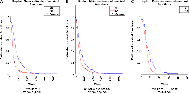
Using the discriminant function based on the TCGA Agilent data, discriminant values were computed for all samples based on Z-scores for TCGA Agilent, TCGA Affymetrix, and Tothill data sets. This was done for all the four cases: OS with tight prefiltering, PFS with tight prefiltering, OS with loose prefiltering, and PFS with loose prefiltering. Patients were divided into two groups: with positive discriminant value and with negative discriminant value. Kaplan–Meier curves were plotted to see whether the survival (OS or PFS, as appropriate) between these two groups was statistically significant. Figures 4 through 7 show the results, including the P-values of obtaining the separation between classes purely by chance.

Figure 4

Kaplan–Meier curves for classifier using OS to define classes and tight prefiltering. P-values are computed using log-rank test.

Figure 5

Kaplan–Meier curves for classifier using OS to define classes and loose prefiltering. P-values are computed using log-rank test.

Figure 6

Kaplan–Meier curves for classifier using PFS to define classes and tight prefiltering. P-values are computed using log-rank test.

Figure 7

Kaplan–Meier curves for classifier using PFS to define classes and loose prefiltering. P-values are computed using log-rank test.

Discussion

We begin with a discussion of the three sets of findings, namely, the ROC curves, the 3 × 3 contingency tables, and the Kaplan–Meier curves. Then, we present an overall discussion.

From the four ROC curves, two broad conclusions can be drawn:

•

Classifiers based on OS to define the classes perform slightly worse than classifiers based on PFS.

•

The classifiers based on loose prefiltering perform better on the training data but slightly worse on the testing data.

For the 3 × 3 contingency tables, where the results of assigning all patients to one of the three categories (SR, MR, and NR) are reported, the broad conclusions are as follows: When OS is used as the clinical parameter, the classifier performs satisfactorily on the TCGA Affymetrix test data; however, it performs poorly on the independent Tothill data set despite the prefiltering of the genes is tight or loose. Therefore, OS does not appear to provide a useful clinical parameter for this purpose. In contrast, if PFS is used as the clinical parameter, then the P-value on the TCGA Affymetrix data set is below machine zero despite the prefiltering is tight or loose. On the independent Tothill data set, the classifier based on tight prefiltering achieves a P-value of 0.0313. When loose prefiltering is used, the classifier based on PFS achieves a P-value of 0.0319. Given that a P-value of 0.05 is widely accepted in biological circles as a benchmark for statistical significance, it can be said that the three-way classification substantially outperforms chance on both the TCGA Affymetrix and Tothill data sets, when PFS is used as the clinical parameter to define the responder classes. Therefore, PFS appears to be a useful clinical parameter that can be used to predict overall patient response.

For the Kaplan–Meier curves, where the entire patient population is divided into two groups, these are the broad conclusions: on the training data consisting of the TCGA Agilent database, the group with a positive score shows a very significant survival advantage over the group with a negative score. However, on the independent validation data set, namely, the Tothill data set, once again the use of OS as the clinical parameter does not lead to satisfactory results.

In contrast, when PFS is used as the clinical parameter, the P-value of the Kaplan–Meier curves using the log-rank test is <0.001 with tight prefiltering and <0.006 with loose prefiltering. Both the values are far lower than the widely accepted threshold of 0.05. Therefore, PFS appears to be a useful clinical parameter for assigning a numerical score to predict patient response.

Now we make some general comments on the outcomes of this paper. The motivation for this research was to determine whether it is possible to predict the response of ovarian cancer patients to front-line platinum chemotherapy using the biomarkers extracted in a purely data-driven fashion via machine learning algorithms. The results are mixed. From the standpoint of considerably outperforming chance, it is unmistakably clear that the biomolecular signatures based on PFS developed here perform spectacularly well on the training data set (TCGA Agilent) as well as one validation data set (TCGA Affymetrix) and also achieve P-values <0.05 on an independent Tothill data set. For the 3 × 3 contingency tables, on an entirely independent validation data set (Tothill), the P-values are ~0.03 if PFS is used as the clinical parameter. Similarly, the P-values of the Kaplan–Meier curves are also <0.006. Therefore, these findings serve to establish that PFS is a very useful clinical parameter that can be used for predicting patient response.

It would be highly desirable to test whether the performance on the Tothill data set could be repeated on other data sets. Unfortunately, in ovarian cancer, there very few large data sets that contain detailed information on the OS and/or PFS of patients. There is one data set, known as the Yoshihara data set, which consists of about 100 samples, and the rest contain fewer than 50 samples. With very few samples, it is not realistic to expect that classifiers would demonstrate a statistically significant improvement over pure chance. Thus, we are forced to remain content with just one independent validation data set, on which the approach leads to good results from the standpoint of statistical significance.

Along similar lines, we have not been able to locate any other molecular signature that can be readily applied to gene expression data, whose predictions can be compared with those given here. The available literature on the topic consists of biomarker panels, that is, lists of genes, but not a numerical procedure for combining the expression values of these genes to assign patients to two or more categories, as is done here.

From the standpoint of being useful in clinical practice, there is considerable scope for improvement. Ideally, the 3 × 3 contingency tables should assist the physician to assign a patient to an appropriate category. If a patient can be said to be an NR with high confidence, then she could straightaway be given alternative therapy. Similarly, if a patient can be said to be an SR with high confidence, the physician can proceed with front-line therapy in an aggressive manner. However, Tables 6 and 7 show that the positive predictive value of these categorizations on the validation data sets is only ~50% or less. Thus, more work is needed to improve these predictions. In other words, an approach can lead to results that are statistically significant while not yet being useful in a clinical setting.

Table 6

Three-way classification based on PFS and tight prefiltering.

LABEL	TCGA AGILENT				TCGA AFFYMETRIX				TOTHILL
Pred./Act.	SR	MR	NR	Total	SR	MR	NR	Total	SR	MR	NR	Total
SR	110	54	24	188	85	63	39	188	15	18	7	40
MR	59	66	62	189	61	62	63	189	20	48	20	88
NR	18	67	103	188	40	60	87	188	4	24	15	43
Total	187	187	185	565	186	185	189	565	39	90	42	171
P-Value	P-Value = 0				P-Value = 0				P-Value = 0.0313

Table 7

Three-way classification based on PFS and loose prefiltering.

LABEL	TCGA AGILENT				TCGA AFFYMETRIX				TOTHILL
Pred./Act.	SR	MR	NR	Total	SR	MR	NR	Total	SR	MR	NR	Total
SR	114	58	16	188	84	60	43	187	12	22	6	40
MR	62	66	59	187	64	64	58	186	23	46	19	88
NR	11	63	114	188	38	61	88	187	4	22	17	43
Total	187	187	189	563	186	185	189	560	39	90	44	171
P-Value	P-Value = 0				P-Value = 0				P-Value 0.0319

One of the objectives of the present paper was to compare OS with PFS as the clinical parameter to categorize a patient. It would appear a priori that OS is a more reliable parameter because there is absolutely no ambiguity about the time of death of a patient (assuming that the clinic has not lost track). On the other hand, as pointed out earlier, the actual date of tumor progression lies somewhere between the reported date of tumor progression and the date of the previous checkup. Therefore, it is surprising that in all the various tests performed, the classifiers based on PFS as the clinical parameter outperform the ones based on OS. One possible explanation is that OS is determined as a whole host of factors, such as age and grade of tumor not just by the gene expression level, and in this sense, PFS is more robust against variations in these additional factors. However, this hypothesis needs to be assessed by gynecological oncologists. Furthermore, it may be desirable to enlarge the set of features beyond gene expression levels by also including other factors, such as age and grade of tumor. For such a study to be meaningful, the number of tumors needs to be an order of magnitude greater than 565, which is available in the TCGA data set.

The predictive features generated in this paper are obtained by using the lone star algorithm,¹⁸ which does not make any use of pathway information or any other contextual information about various features. Other work carried out by a subset of the authors has led to an algorithm known as “phixer” that can be used to reverse engineer whole-genome context-sensitive gene interaction networks. Future work by our research team would consist of combining these two algorithms so as to choose features that are both highly predictive and also interpretable in terms of biological pathways.

A recent paper on melanoma²³ suggests that there are different evolutionary trajectories for different subtypes. This is a very significant observation, and it is likely that similar conclusions might apply to other forms of cancer, though this is yet to be established. If differences in patient responses in ovarian cancer were to be the result of tumors in different patients following different evolution trajectories, the complexity of the disease would increase enormously; in turn, this would make it more difficult to apply machine learning methods of the type used in the present paper.

Conclusions

In this paper, we have proposed a methodology for grouping ovarian cancer patients into three categories, referred to here as SRs, MRs, and NRs, in terms of their response to front-line platinum chemotherapy. We have also developed an approach for grouping patients into two groups in such a way that one group has a statistically significant survival advantage over the other. While both approaches achieve P-values far below the widely accepted threshold of 0.05, further work is required to make this approach useful in a clinical setting.

Author Contributions

Conceived the problem and formulated the approach: MAW, MV. Analyzed the data and carried out the computations: BM, EA, NS. Wrote all drafts of the manuscript: BM, MV. Contributed to the writing of the manuscript: KAB, AU. Made critical revisions and approved the final version: KAB, MAW. All authors reviewed and approved of the final manuscript.

References

Siegel

R.L.

Miller

K.D.

Jemal

Cancer statistics, 2015. CA Cancer J Clin. 2015; 65(1): 5–29.

Cai

Yang

Prognostic significance of several biomarkers in epithelial ovarian cancer: a meta-analysis of published studies. J Cancer Res Clin Oncol. 2013; 139(8): 1257–77.

The Cancer Genome Atlas Research Network. Integrated genomic analyses of ovarian carcinoma. Nature. 2011; 474: 609–15.

Hartmann

L.C.

K.H.

Linnette

G.P.

Gene expression profiles predict early relapse in ovarian cancer after platinum-paclitaxel chemotherapy. Clin Cancer Res. 2005; 11: 2149–55.

Tothill

R.W.

Tinker

A.V.

George

Novel molecular subtypes of serous and endometrioid ovarian cancer linked to clinical outcome. Clin Cancer Res. 2008; 14: 5198–208.

Varga

Deniz

Schwentner

Wiesmüller

Ovarian cancer: in search of better marker systems based on DNA repair defects. Int J Mol Sci. 2013; 14(1): 640–73.

Wilson

A.J.

Liu

A.Y.

Roland

J.T.

TR3 modulates platinum resistance in ovarian cancer. Cancer Res. 2013; 73(15): 4758–69.

Smoter

Bodnar

Grala

Tau protein as a potential predictive marker in epithelial ovarian cancer patients treated with paclitaxel/platinum first-line chemotherapy. J Exp Clin Cancer Res. 2013; 32: 25.

Kavallaris

Kuo

D-S

Burkhart

C.A.

Taxol-resistant epithelial ovarian tumors are associated with altered expression of specific β-tubulin isotypes. J Clin Invest. 1997; 100(5): 1282–93.

10.

Roque

D.M.

Belone

Buza

Class iii β-tubulin overexpression in ovarian clear cell and serous carcinoma as a maker for poor overall survival after platinum/taxane chemotherapy and sensitivity to patupilone. Am J Obstet Gynecol. 2013; 209(1): 62.e1–62.e9.

11.

Han

Huang

Xiao

Integrated analysis of gene expression profiles associated with response of platinum/pactitaxel-based treatment in epithelial ovarian cancer. PLOS One. 2012; 7(12): e52745.

12.

Denkert

Budczies

Darb-Esfahani

A prognostic gene expression index in ovarian cancer – validation across different independent data sets. J Pathol. 2009; 218: 273–80.

13.

Sabatier

Finetti

Cervera

Birnbaum

Bertucci

Gene expression profiling and prediction of clinical outcome in ovarian cancer. Crit Rev Oncol Hematol. 2009; 72(2): 98–109.

14.

Kang

D'Andrea

A.D.

Kozono

A DNA repair pathway-focused score for prediction of outcomes in ovarian cancer treated with platinum-based chemotherapy. J Natl Cancer Inst. 2012; 104(9): 670–81.

15.

Kang

Sun

H.Y.

Zhou

R.M.

Wang

DNA repair gene associated with clinical outcome of epithelial ovarian cancer treated with platinum-based chemotherapy. Asian Pac J Cancer Prev. 2013; 14(2): 941–6.

16.

Yang

Khan

Sun

Association of BRCA1 and BRCA2 mutations with survival, chemotherapy sensitivity, and gene mutator phenotype in patients with ovarian cancer. J Am Med Assoc. 2011; 306(14): 1557–65.

17.

Waldron

Haibe-Kains

Culhane

A.C.

Comparative meta-analysis of prognostic gene signatures for late-stage ovarian cancer. J Natl Cancer Inst. 2014; 106(5): dju049.

18.

Ahsen

M.E.

Singh

N.K.

Boren

Vidyasagar

White

M.A.

A new feature selection algorithm for two-class classification problems and application to endo-metrial cancer. In: Proceedings, IEEE Conference on Decision and Control. Maui, HI: 2012: 2976–82.

19.

Vidyasagar

Machine learning methods in cancer biology. Proc Royal Soc A. 2014; 470: 20140081.

20.

Bradley

P.S.

Mangasarian

O.L.

Feature selection via concave minimization and support vector machines. In: Machine Learning: Proceedings of the Fifteenth International Conference (ICML ‘98). San Francisco, CA: Morgan Kaufmann; 1998: 82–90.

21.

Guyon

Weston

Barnhill

Vapnik

Gene selection for cancer classification using support vector machines. Machine Learn. 2002; 46: 389–422.

22.

Meinshausen

Bühlmann

Stability selection. J Royal Statist Soc B. 2010; 72: 417–83.

23.

Shain

A.H.

Yeh

Kovalyshyn

The genetic evolution of melanoma from precursor lesions. N Engl J Med. 2015; 373(20): 1926–36.