Bayesian ABC-MCMC Classification of Liquid Chromatography–Mass Spectrometry Data

Abstract

Proteomics promises to revolutionize cancer treatment and prevention by facilitating the discovery of molecular biomarkers. Progress has been impeded, however, by the small-sample, high-dimensional nature of proteomic data. We propose the application of a Bayesian approach to address this issue in classification of proteomic profiles generated by liquid chromatography-mass spectrometry (LC-MS). Our approach relies on a previously proposed model of the LC-MS experiment, as well as on the theory of the optimal Bayesian classifier (OBC). Computation of the OBC requires the combination of a likelihood-free methodology called approximate Bayesian computation (ABC) as well as Markov chain Monte Carlo (MCMC) sampling. Numerical experiments using synthetic LC-MS data based on an actual human proteome indicate that the proposed ABC-MCMC classification rule outperforms classical methods such as support vector machines, linear discriminant analysis, and 3-nearest neighbor classification rules in the case when sample size is small or the number of selected proteins used to classify is large.

Introduction

Recent advances in high-throughput technologies in proteomics promise to revolutionize cancer treatment and prevention by facilitating the discovery of molecular biomarkers, which can be used to improve diagnosis, guide targeted therapy, and monitor therapeutic response. ¹ Among all high-throughput proteomic technologies, mass spectrometry has increasingly become the method of choice for the analysis of complex protein samples. ² High molecular specificity and excellent detection sensitivity explain the widespread adoption of mass spectrometry (MS)-based proteomics as a popular tool for the identification and quantification of the composition of complex proteome mixtures.

However, to date, the rate of discovery of successful biomarkers is still unsatisfactory. In addition to challenges such as the high dynamic range of proteins ³ and inaccurate protein quantification, ⁴ an important impediment to progress is that, in clinical applications of mass spectrometry, the number of samples available is extremely small, whereas mass spectra contain hundreds of thousands of intensity measurements with signals generated by thousands of proteins/peptides. This small-sample, high-dimensionality problem requires the experiment and analysis to be carefully designed and validated in order to arrive at statistically meaningful results. Through model-based approaches and simulation using ground-truthed synthetic data, the problem of biomarker discovery can be studied and evaluated.

In this paper, we propose the application of a Bayesian approach to address the small-sample, high-dimensionality problem in the classification of proteomic profiles generated by liquid chromatography–mass spectrometry (LC-MS). Our approach relies on the detailed LC-MS experiment pipeline model developed in Ref. 5, as well as on the theory of the optimal Bayesian classifier (OBC), proposed in Ref. 6. However, the complexity of the LC-MS experiment, involving steps of sample preparation, protein digestion, peptide ionization, peptide detection, and protein quantification, implies that the likelihood function for the LC-MS model is exceedingly complex, requiring the application of a likelihood-free Bayesian approach. In this paper, we apply a new likelihood-free methodology called approximate Bayesian computation (ABC). ⁷ The basic ABC rejection sampling method generates candidate parameters by sampling from the prior distribution and creates a model-based simulated dataset. If the dataset conforms to the observed dataset, the candidate can be retained as a sample from the posterior distribution. Thus, one can avoid evaluating the likelihood function, which is essential for classical Bayesian posterior simulation methods. The ABC approach can also be implemented via a combination of rejection sampling and Markov chain Monte Carlo (MCMC) sampling. ⁸

The detailed implementation of our approach involves first the prior calibration of the hyperparameters of the LC-MS model using an ABC approach via rejection sampling and then using the ABC method implemented via an MCMC procedure to obtain samples from the posterior distribution of the protein concentrations, which are used to approximate the OBC using Monte Carlo integration and kernel smoothing. Numerical experiments using synthetic LC-MS data based on an actual human proteome indicate that the ABC-MCMC classification rule outperforms classical methods such as support vector machines (SVMs), linear discriminant analysis (LDA), and 3-nearest neighbor (3NN) classifiers in the case when sample size is small or the number of selected proteins used to classify is large. We also quantify the effect of experimental parameters such as the coefficient of variation (noise) and instrument peptide efficiency factor on classification accuracy.

The paper is organized as follows. The “LC-MS Model” section surveys the LC-MS model proposed in Ref. 5, which is the basis for our inference approach. The ‘ABC-MCMC Classification Framework” section describes in detail the algorithms for prior calibration, sampling from the posterior, and computation of the ABC-MCMC classifier. The “Numerical Experiments” section presents the results of a numerical experiment using synthetic LC-MS data corresponding to a subset of the human proteome. Finally, the “Conclusion” section brings concluding remarks.

LC-MS Model

Here, we describe briefly the label-free LC-MS model proposed in Ref. 5. Two sample classes are considered, control (class 0) and treatment (class 1). There are n sample profiles from each class, sharing N_pro protein species from a specified proteome, which is typically input into the model as a FASTA file. As argued in Ref. 9, protein concentration in the control sample is best described as a Gamma distribution,

$${\gamma }_l=\Gamma \left(k,\theta \right),\hspace{0.17em}l=1,2,\cdots ,N_{pro},$$

(1)

where the shape k and scale θ parameters are assumed to be uniform random variables, such that k ~ Unif(k_low, k_high) and θ ~ Unif(θ_low, θ_high). The values for k_low, k_high, θ_low, and θ_high were chosen to adequately reflect the dynamic range of protein abundance levels (see the “Numerical Experiments” section).

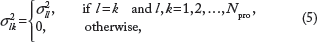
According to whether there is a significant difference in abundance between control and treatment populations, proteins are divided into biomarker (differentially expressed) proteins and background (not differentially expressed) proteins. The difference in abundance for biomarker proteins is quantified by the fold change,

$$f_l=\{\begin{array}{cc}{a}_{l,}& \text{if the }l\text{th}\hspace{0.17em}\text{protein}\hspace{0.17em}\text{is}\hspace{0.17em}\text{overexpressed,}\\ 1/a_l& \text{if}\hspace{0.17em}\text{the}\hspace{0.17em}l\text{th}\hspace{0.17em}\text{protein}\hspace{0.17em}\text{is}\hspace{0.17em}\text{underexpressed,}\\ 1,& \text{otherwise}.\end{array}$$

(2)

The multivariate Gaussian distribution is recommended as the model for protein concentration variations in each class. ¹⁰ Accordingly, the protein expression level for the lth protein in the jth sample profile is modeled as

$$c_{lj}^{pro}=\{\begin{array}{cc}\mathcal{N}\left(\left[{\gamma }_{1,}{\gamma }_2,\dots ,{\gamma }_{N_{pro}}\right],\sum \right)& \text{if}\hspace{0.17em}j\in \hspace{0.17em}\text{class}\hspace{0.17em}0,\\ \mathcal{N}\left(\left[{\gamma }_1{f}_1,{\gamma }_2{f}_2,\dots ,{\gamma }_{N_{pro}}{f}_{N_{pro}}\right],\sum \right)& \text{if}\hspace{0.17em}j\in \hspace{0.17em}\text{class}\hspace{0.17em}1.\end{array}$$

(3)

In this paper, we assume a diagonal covariance matrix $\sum ={\left[{\sigma }_{lk}^2\right]}_{N_{pro}\times N_{pro}}$ such that protein concentrations are mutually independent (the results will still be approximately valid as long as the proteins are only weakly correlated):

$$\sum =\left[\begin{array}{cccc}{\alpha }_{11}^2& 0& \cdots & 0\\ 0& {\alpha }_{22}^2& \cdots & 0\\ ⋮& ⋮& \ddots & ⋮\\ 0& 0& \cdots & {\alpha }_{N_{pro}{N}_{pro}}^2\end{array}\right]$$

(4)

where

$${\sigma }_{lk}^2=\{\begin{array}{cc}{\sigma }_{ll}^2,& \text{if}\hspace{0.17em}l=k\hspace{0.17em}and\hspace{0.17em}l,k=1,2,\cdots ,N_{pro}\\ 0,& \text{otherwise,}\end{array}$$

(5)

and

$$\begin{array}{cc}{\sigma }_{ll}^2=\phi \times {\gamma }_l^2,& l=1,2,\cdots ,N_{pro}.\end{array}$$

(6)

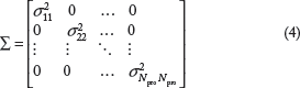
The coefficient of variation ϕ is calibrated based on the observed data.

In order to perform in silico tryptic digestion of the protein samples, we use the peptide mixture model from openMS. ¹¹ Let ω _i be the set of all proteins that contain the ith peptide. If there are N_pep peptide species, in total, across all proteins in a given sample, then their molar concentrations are given as

$$\begin{array}{ccc}{c}_{ij}^{pep}=\sum _{k\in {\Omega }_i}{c}_{kj}^{pro},& i=1,2,\cdots ,N_{pep},& j=1,2,\cdots ,2n.\end{array}$$

(7)

In general, ion abundance in MS data bears the signature of the concentration of a peptide type, say i in sample j. Taking measurement uncertainty factors in consideration, one may envisage that the expected readout μ _ij of the abundance of said peptide can be modeled as,

$$\begin{array}{ccc}{\mu }_{ij}=c_{ij}^{pep}{e}_i\kappa ,& i=1,2,\cdots ,N_{pep}& j=1,2,\cdots ,\cdots ,2n,\end{array}$$

(8)

where e _i denotes the peptide efficiency factor and κ represents the LC-MS instrument response factor. ⁵

The true peptide abundance differs from its readout due to noise. Accordingly, the actual abundance of a peptide v _ij is modeled as v _ij = μ _ij + ∊ _ij , where ∊ _ij is additive Gaussian noise and follows the distribution

$$\begin{array}{ccc}{\in }_{ij}~\mathcal{N}\left(0,\alpha {\mu }_{ij}^2+\beta {\mu }_{ij}\right),& i=1,2,\cdots ,N_{pep},& j=1,2,\cdots ,2n,\end{array}$$

(9)

where α and β specify the quadratic dependence of the noise variance on the expected abundance.^5,12

Peptide signals observed in mass spectra are in fact the result of true signals with interfering noise signals and also signals from other peptides. Therefore, the signal-to-noise ratio (SNR) affects the true positive rate (TPR) greatly. To take account of this, we describe the SNR as

$$SNR=\frac{E{\left[\upsilon \right]}^2}{Var\left(\upsilon \right)}=\frac{1}{\alpha +\frac{\beta }{\mu }}.$$

(10)

Taking interfering signals in consideration, the TPR of peptides is defined as

$$\text{TPR}=\left(t\times {\text{SNR}}^p+b\right)\times o_{ij},$$

(11)

where 0 _ij is an overlapping factor. If algorithms like NITPICK, BPDA, and BPDA2d are used, then 0 _ij ≈ 1. ⁵

Finally, we consider in our model three peptide filters, in order: (1) nonunique peptides present in more than one protein of the proteome in study are discarded; (2) peptides with missing value rates greater than 0.7 are discarded; and (3) among the remaining peptides, those having correlation larger than 0.6 with all other peptides are kept.

The MS1 output provides information about detected peptides, their abundances, and related characteristics. The process of filtering these data and compiling the parent protein abundances from the raw peptide data is called protein abundance roll-up. To obtain the identities of the parent proteins from captured peptide sequence information, one will often use a second round of MS and search available MS/MS (MS2) databases. Alternatively, the accurate mass and time approach matches peptides to databases using the monoisotopic mass and elution time predictors, obviating the need of a second step of MS. ¹³ We will assume here that data are available in the form of rolled-up abundances, whereby the readout of protein l in sample j can be written as

$$\begin{array}{ccc}{x}_{ij}=\frac{1}{\kappa n_l}\sum _{i\in {\mathcal{N}}_l}{\upsilon }_{ij},& l=1,2,\dots ,N_{pro},& j=\end{array}1,2,\dots ,2n,$$

(12)

where κ is the instrument response factor, N _l is the set of all peptides present in protein l that are retained after the filtering scheme described in the previous paragraph, and n _l is the number of peptides in set N _l . The protein abundance is set to zero when less than two peptides pass the previous filters.

ABC-MCMC Classification Framework

Bayesian analysis for complex models used in recent applications involve intractable likelihood functions, which has prompted the development of new algorithms generally called approximate Bayesian computation (ABC). In this approach, one generates candidate parameters by sampling from the prior distribution and creating a model-based simulated dataset. If the dataset conforms to the observed dataset, the candidate can be retained as a sample from the posterior distribution. Thus, one can avoid evaluating the likelihood function, which is essential for classical Bayesian posterior simulation methods. The ABC approach can be implemented via rejection sampling, MCMC, and sequential Monte Carlo methods. ⁸ Utilizing the LC-MS proteomics model described in the last section, we first do prior calibration of the hyperparameters using an ABC approach via rejection sampling, and then use the ABC method implemented via an MCMC procedure to obtain samples from the posterior distribution of the protein concentrations in order to derive the ABC-MCMC classifier for LC-MS data.

Overview of the inference procedure

The sample data S = S₀ ⋓ S₁ consist of two subsamples S₀ and S₁ corresponding to the control group (eg, healthy volunteers) and treatment group (eg, cancer patients), respectively, where each subsample contains n protein abundance profiles. Given the sample data, the total number of proteins N_pro is reduced via feature selection (eg, ranking by the two-sample t-test statistic) to a tractable number d of selected proteins. According to the adopted LC-MS model, described in the “LC-MS Model” section, the protein abundance profiles are a function of the baseline protein concentration vector γ = (γ₁, …, γ _d , (b) the prior hyperparameters k, θ, ϕ, f , consisting of shape and scale parameters of the Gamma distribution in (1), the fold change parameters in (2), and the coefficient of variation in (6); and (c) the LC-MS instrument-related parameters κ, α, β, e , b, t, p, which are assumed to be known for a given instrument (see Table 1 for the value of these parameters in our numerical experiment). Figure 1 displays the relationship among these various parameters.

Figure 1

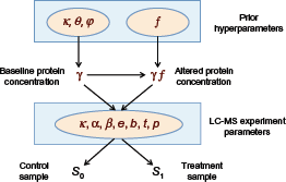
Relationship among all parameters of the LC-MS model (see text).

Table 1

LC-MS parameters used in the experiment.

PARAMETER	SYMBOL	VALUE/RANGE
Instrument response	κ	5
Noise severity	α, β	0.03, 3.6
Peptide efficiency factor	e i	[0.1–1]
Peptide detection algorithm	b, t, p	0,0.0016,2

Our approach consists of treating γ as the hidden parameter vector, posterior samples of which are obtained using an ABC-MCMC sampling method, after a step of calibration of the hyperparameters using ABC rejection sampling. The samples from the posterior allow us to calculate the OBC for the problem. All these steps are described in detail in the sequel.

Algorithm 1

Prior calibration of k, θ, and ϕ using ABC rejection sampling.

1. 1.

   Generate M_cal triplets of parameters of {k ^(t) ,θ ^(t) ,ϕ ^(t) } such that,

   $$\begin{array}{l}{k}^{\left(t\right)}~Unif\left(k_{low},k_{high}\right),{\theta }^{(t)}~Unif\left({\theta }_{low},{\theta }_{high}\right),\\ {\phi }^{\left(t\right)}~Unif\left({\phi }_{low},{\phi }_{high}\right)\end{array}$$
   for t = 1,…, M_cal.

2. 2.

   Simulate a control sample set $S_0^{\left(t\right)}$ of size n for each triplet {k ^(t) ,θ ^(t) ,ϕ ^(t) } for t = 1, 2,…, M_cal.

3. 3.

   Accept the triplet {k ^(t) ,θ ^(t) ,ϕ ^(t) } if | T | < ∊, for t = 1,…,M_cal, where |·| denotes the Euclidean norm and T denotes the vector sample mean.

4. 4.

   Let $\mathcal{A}=\left\{\left\{k^1,{\theta }^1,{\phi }^1\right\},\cdots ,\left\{k^{n_a},{\theta }^{n_a},{\phi }^{n_a}\right\}\right\}$ be the set of all accepted triplets. The calibrated k can be approximated as follows

   $$k_{cal}={\int }_{k_{low}}^{k_{high}}kp\left(k|S_n\right)dk\approx \frac{1}{n_a}\sum _{a=1}^{n_a}{k}^a.$$

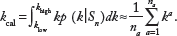
Similar Monte Carlo integrations are performed to calculate θ_cal and ϕ_cal.

Prior calibration via ABC rejection sampling

Calibration of the hyperparameters k, θ, ϕ, f is accomplished using the ABC rejection sampling method. Unlike Knight et al. ¹⁴ , who proposed using discarded features to perform prior calibration for an MCMC implementation of the OBC, here we use the selected features, as we need to calibrate the fold change as well, which is specific to each selected protein.

First, we calibrate k, θ, and ϕ using the control sample only, since these parameters are common across control and treatment populations and f has not been calibrated yet. The procedure used is displayed in Algorithm 1. In this algorithm, ∊ is the error tolerance. It has been proved ⁷ that smaller ∊ gives better approximation of the posterior p(k|S _n ). However, this must be balanced against the possibility that $P\left(\Vert T\left(S_0^{\left(t\right)}\right),T\left(S_0\right)\Vert <\in \right)\approx 0$ , which would prevent convergence to the posterior.

Next we calibrate the fold change parameter f = (f₁,…,f _d ) for each selected protein. If sample size is large (n > 50) then the simple sample estimate

$$f_{l,cal}=\frac{T_l\left(S_1\right)}{T_l\left(S_0\right)},\hspace{0.17em}for\hspace{0.17em}l=1,\cdots ,d,$$

(13)

where T _l denotes the sample mean for the lth selected protein only, is fairly accurate, and may be used as the prior calibration. However, for smaller sample sizes, we follow the steps enumerated below in Algorithm 2.

Posterior sampling via an ABC-MCMC procedure

After prior calibration, we would like now to draw samples from the posterior distribution of the protein baseline expression vector γ = (γ₁,…,γ _d ), namely, p(γ| S _n )∝ p(S _n | γ)p(γ), in order to derive the OBC. In our case, no closed-form expressions for either the likelihood function or posterior distribution exist, so Bayesian analysis is performed using an ABC-MCMC procedure, described in Algorithm 3. After a burn-in interval of t _s time steps, the Markov chain is assumed to have become stationary, and ${\gamma }^{\left(t_s+1\right)},\dots ,{\gamma }^{\left(t_s+M\right)}$ may be considered to be samples from the baseline expression posterior distribution p(γ|y=0,S _n ), while ${\gamma }^{\left(t_s+1\right)}{f}_{cal},\dots ,{\gamma }^{\left(t_s+M\right)}{f}_{cal}$ (where vector multiplication is defined as componentwise multiplication) maybe taken to be samples from the altered expression posterior distribution p(γ|y=1,S _n ).

Algorithm 2

Prior calibration of f _l , l = 1,…, d, using ABC rejection sampling.

1. 1.

   Generate M_cal baseline expression values ${\gamma }_l^{\left(t\right)}~\Gamma \left(k_{cal},{\theta }_{cal}\right)$ for t = 1,…,M_cal.

2. 2.

   Simulate a control sample $S_0^{\left(t\right)}$ of size n using the baseline expression mean ${\gamma }_l^{\left(t\right)}$ , for t = 1,…,M_cal (in fact, only the abundances for the lth protein need to be generated).

3. 3.

   Accept ${\gamma }_l^{\left(t\right)}$ if $T_l\left(S_0^{\left(t\right)}\right)-T_l\left(S_0\right)|<{\in }_1$ and $p_l\left(S_0^{\left(t\right)},S_0\right)>1-{\in }_2$ , where T _l denotes the sample mean and ρ _l denotes the sample correlation for the abundances of the lth protein only.

4. 4.

   Generate M_cal fold change parameters $f_l^{\left(t\right)}$ such that If T _l (S₁)/T _l (S₀) ≥ 1, then $f_l^{\left(t\right)}~Unif\left({\alpha }_{low},{\alpha }_{high}\right)$ , If T _l (S₁)/T _l (S₀) < 1, then $f_l^{\left(t\right)}~Unif\left(1/{\alpha }_{high},{\alpha }_{low}\right)$ , for t = 1,…, M_cal.

5. 5.

   Simulate a treatment sample $S_1^{\left(t\right)}$ of size n using the altered expression mean $f_l^{\left(t\right)}{\gamma }_l^{\left(t\right)}$ , for t = 1, 2,…, M_cal (in fact, only the abundances for the lth protein need be generated).

6. 6.

   Accept $f_l^{\left(t\right)}{\gamma }_l^{\left(t\right)}$ if $\left|T_l\left(S_1^{\left(t\right)}\right)-T_l\left(S_l\right)\right|<{\in }_1$ and $\rho \left(S_1^{\left(t\right)},S_1\right)>1-{\in }_2$ .

7. 7.

   Let $n_a^0$ be the number of accepted baseline expression means in step 3 and let $n_a^1$ be the number of accepted altered expression means in step 6. Define ${\lambda }^0=n_a^0/M_{cal}$ , the rate of acceptance of control means, ${\lambda }^0=n_a^1/M_{cal}$ , the rate of acceptance of treatment means.

8. 8.

   If λ⁰ > λ¹ then assign f_l,cal = 1 (ie, background protein) and return from the algorithm.

9. 9.

   Otherwise, f_cal,l ≠ 1 (ie, marker protein). For all the accepted altered expression means, we perturb each of the fold changes $f_l^{*}=f_l+N_l$ , where N _l is zero-mean Gaussian noise with a small variance. With these perturbed fold changes, we again apply the ABC rejection algorithm, this time with error tolerances, ${\in }_1^{\text{'}}<{\in }_1$ and ${\in }_2^{\text{'}}<{\in }_2$ .

10. 10.

    The mean of all accepted fold change parameters in step 9 is a reasonably accurate fold changed f_cal for the given protein.

Optimal Bayesian classifier

Let ψ: R ^d ↠ {0, 1} be a classifier that takes a protein abundance profile X ∊ R ^d into one of the two labels 0 or 1, which code for the control (baseline expression) and treatment (altered expression) populations, respectively. The error of the classifier is the probability of a mistake given the sample data:

$$\epsilon \left[\psi \right]=P\left(\psi \left(X\right)\ne Y|S\right),$$

(14)

where Y ∊ {0, 1} denotes the true label corresponding to X.

Algorithm 3

Posterior sampling of γ using an ABC-MCMC procedure.

1. 1.

   Generate γ ⁽⁰⁾ = (γ₀, γ₁, …, γ _d ) such that γ _l ~ γ(k, θ), for l = 1, 2, …, d.

2. 2.

   Simulate control and treatment samples $S_0^{\left(0\right)}$ and $S_1^{\left(0\right)}$ of size n using γ ⁽⁰⁾ and γ ⁽⁰⁾ f _cal, respectively (where vector multiplication is defined as componentwise multiplication).

3. 3.

   Accept γ ⁽⁰⁾ if $\Vert T\left(S_0^{\left(0\right)}-T\left(S_0\right)\right)\Vert <{\in }_0$ and $\Vert T\left(S_1^{\left(0\right)}-T\left(S_1\right)\right)\Vert <{\in }_1$ , otherwise repeat steps 1 and 2 until the condition is met.

For t = 0,1,…, t _s , t_s+1,…,t _s + M where t _s is the burn-in period, repeat:

1. 4.

   Generate γ ^(t+1) ~ g(γ; γ ^(t) ), where the proposal density g(γ; γ ^(t) ) is multivariate Gaussian ℕ _d (γ ^(t) ,σ ² I ^d ), with a small variance σ ² .

2. 5.

   Simulate control and treatment samples $S_0^{\left(t+1\right)}$ and $S_1^{\left(t+1\right)}$ of size n using γ ^(t+1) and γ ^(t+1) f _cal, respectively.

3. 6.

   Let $q=\{\begin{array}{cc}\min \left(1,\frac{p\left({\gamma }^{\left(t+1\right)}g{\gamma }^{\left(t\right)};{\gamma }^{\left(t+1\right)}\right)}{p\left({\gamma }^{\left(t\right)}\right)g\left({\gamma }^{\left(t+1\right)};{\gamma }^{\left(t\right)}\right)}\right),& \begin{array}{l}\text{if}\Vert T\left(s_0^{\left(t+1\right)}\right)-T\left(s_0\right)\Vert <{\in }_0\\ \text{and}\hspace{0.17em}\Vert T\left(s_1^{\left(t+1\right)}\right)-T\left(s_1\right)\Vert <{\in }_1\end{array}\\ 0& \text{otherwise,}\end{array}$ where p(·) is the Gamma prior for protein baseline expression.

4. 5.

   Accept γ ^(t+1) with probability q, or let γ ^(t+1) = γ ^(t) with probability 1 – q.

Now, consider a Bayesian setting, where the joint distribution of ( X,Y ) depends on a random parameter vector θ. In this case, the classification error ∊ _θ [ψ] also becomes a random variable, as a function of θ. The expected value of the classification error over the posterior distribution of fi becomes the quantity of interest:

$$E_{\theta |S}\left[{\epsilon }_{\theta }\left[\psi \right]\right]=E_{\theta |S}\left[P\left(\psi \left(X\right)\ne Y|\theta ,S\right)\right].$$

(15)

The OBC ⁶ is the classifier that minimizes the quantity in (15):

$${\psi }_{OBC}=\underset{\psi \in C}{\arg \min }{E}_{\theta |S}\left[{\epsilon }_{\theta }\left[\psi \right]\right],$$

(16)

where C is the space of classifiers. It was shown in Ref. 6 that the OBC is given by

$${\psi }_{OBC}\left(x\right)=\{\begin{array}{cc}1,& \text{if}\hspace{0.17em}E\left[c|S\right]p\left(x|Y=1,S\right)>\left(1-E\left[c|S\right]\right)p\left(x|Y=0,S\right),\\ 0,& \text{otherwise}\end{array}$$

(17)

where c = P(Y = 1 | θ ) is the prior probability of class 1, and

$$\begin{array}{cc}p\left(x|Y=y,S\right)={\int }_{\Theta }p\left(x|\theta ,Y=y,S\right)p\left(\theta |Y=y,S\right)d\theta ,& y=0,1,\end{array}$$

(18)

are the effective class-conditional densities.

In the present case of the LC-MS model discussed in the “LC-MS Model” section, the random parameter vector 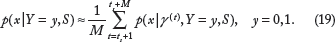θ corresponds to the baseline expression vector γ. We approximate the integral in (18) using the MCMC samples ${\gamma }^{\left(t_s+1\right)},\cdots ,{\gamma }^{\left(t_s+M\right)}$ from the posterior distribution of γ, obtained with Algorithm 3:

$$\begin{array}{cc}p\left(x|Y=y,S\right)\approx \frac{1}{M}\sum _{t=t,+1}^{t_s+M}p\left(x|{\gamma }^{\left(t\right)},Y=y,S\right),& y=0,1.\end{array}$$

(19)

Now, the densities p( x | γ ^(t) ,Y = y, S), y = 0, 1, cannot be directly determined for the LC-MS model, and hence we approximate them using a kernel-based approach. For each MCMC sample γ ^(t) , we simulate control and treatment samples $S_0^{\left(0\right)}$ and $S_1^{\left(0\right)}$ of size n based on γ ^(t+1) and γ ^(t+1) f _cal, respectively. Let $S_0^{\left(t\right)}=\left\{x_1^{\left(t\right)},\cdots ,x_n^{\left(t\right)}\right\}$ and $S_1^{\left(t\right)}=\left\{x_{n+1}^{\left(t\right)},\cdots ,x_{2n}^{\left(t\right)}\right\}$ . Then

$$\begin{array}{cc}p\left(x|{\gamma }^{\left(t\right)},Y=y,S\right)\approx \frac{1}{n}\sum _{t=ny+1}^{ny+n}\frac{1}{h^d}K\left(\frac{x-x_j^{\left(t\right)}}{h}\right),& y=0,1,\end{array}$$

(20)

where K is a zero-mean, unit-covariance, multivariate Gaussian density, and h > 0 is a suitable kernel bandwidth parameter.

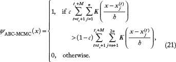
In addition, we will assume c to be known (eg, from epidemiological data) and fixed, so E[c | S] = c. After some simplification, the resulting OBC, which we call an ABC-MCMC Bayesian classifier, is a kernel-based classifier given by

$$\begin{array}{cc}1,& if\hspace{0.17em}c\hspace{0.17em}\sum _{t=t,+1}^{t_s+M}\sum _{j=1}^{n}K\left(\frac{x-x_j^{\left(t\right)}}{h}\right)\\ & >\left(1-c\right)\sum _{t=t,+1}^{t_s+M}\sum _{j=n+1}^{2n}K\left(\frac{x-x_j^{\left(t\right)}}{h}\right),\\ 0,& \text{otherwise}.\end{array}$$

(21)

Numerical Experiments

We demonstrate the application of the proposed ABC-MCMC classification rule to synthetic LC-MS data generated from a subset of the human proteome, containing around 4000 drug targets, which was compiled as a FASTA file from DrugBank ¹⁵ – this is the same proteome that was used in the numerical experiments of Ref. 5 – and compare its performance against that of popular classification rules: linear support vector machines, LDA, and 3NN. ¹⁶ As our interest is on small-sample performance, we selected methods that are simple and known to perform well with small samples and avoid overfitting: linear SVMs are sophisticated methods widely used in the pattern recognition and machine learning communities, which displays minimal overfitting, while LDA and 3NN are classical methods that are well known to have superior small-sample performance. ¹⁷

We select randomly among these data 500 proteins to play the role of background proteins, along with 20 proteins to serve as biomarkers. Synthetic LC-MS protein abundance data were generated using realistic sample preparation, LC-MS instrument characteristics, and protein quantification parameters – see Table 1. These are the “LC-MS experiment parameters” of Figure 1, which are assumed to be known and are held constant throughout the simulation. (For the peptide efficiency factor, values uniformly distributed in the indicated range are randomly generated for each peptide, and then held constant.) As argued in Ref. 5, the values and ranges adopted in Table 1 adequately represent the peptide mixture, peptide abundance mapping, peptide detection and identification, and protein abundance roll-up that is typical in an LC-MS workflow.

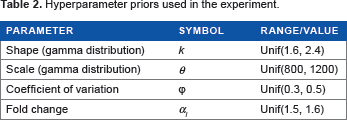
The hyperparameter priors for k, θ, ϕ, f are the uniform distributions shown in Table 2 (except where noted below). The lower and upper bounds of each interval are chosen while keeping in consideration that, in practice, the dynamic range of protein expression level has approximately 4 orders of magnitude. ⁵ The synthetic sample data were generated using the middle point of each interval as parameters: k = 2, θ = 1000, ϕ = 0.4, and α _l = 1.55 (again, except where noted below).

Table 2

Hyperparameter priors used in the experiment.

PARAMETER	SYMBOL	RANGE/VALUE
Shape (gamma distribution)	k	Unif(1.6, 2.4)
Scale (gamma distribution)	θ	Unif(800, 1200)
Coefficient of variation	ϕ	Unif(0.3, 0.5)
Fold change	α l	Unif(1.5, 1.6)

We consider sample sizes from n = 10 through n = 50 per class, and select d = 3, 5, 8, or 10 proteins from the original 520 proteins using the two-sample t-test (notice that background proteins could be erroneously selected by the t-test, especially for small sample sizes, which makes the experiment realistic).

For the MCMC step, M = 10,000 samples were drawn from the posterior distribution of γ , after a burn-in stage of t _s = 3000 iterations, which confers a high degree of accuracy to the approximation. A constant value c = 0.5 was assumed in (21).

A total of 12 runs of the experiment were run for each combination of sample size, dimensionality, and parameter settings, and the average true error rate for each classification rule was obtained using a large synthetic test set containing 1000 sample points. This is a comprehensive simulation, given the relatively large computational burden required for accurate prior calibration and ABC-MCMC computation.

The root mean square error (RMS) of the test set error estimator, which reflects the expected distance between the estimate and the true error, is bounded by equation (2.29) in Ref. 17 as follows

$$RMS\le \frac{1}{2\sqrt{m}},$$

(22)

where m is the number of test points. With m = 1000, we obtain RMS ≤ 0.016, which is of the order of the differences in average error rates observed in the plots. While not implying statistical significance, this result means that we can assign a large degree of confidence to the comparative results.

Effect of sample size

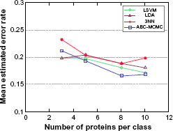
Figure 2 displays the expected error rates of the various classification rules for varying sample size and fixed number of selected proteins d = 8. We can see that, as expected, the expected error rates of all classifiers tend to go down as sample size increases, but the ABC-MCMC classifier has the smallest expected error at small sample sizes. This is in agreement with the predicted superiority of the Bayesian approach in small-sample scenarios. Though the difference in performance among the classification rules may seem to be small, the point to be emphasized is that the ABC-MCMC displays a consistently smaller error rate for small sample sizes.

Figure 2

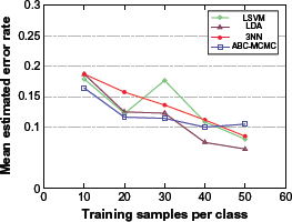
Expected classification error rates for varying sample size and fixed number of selected proteins d = 8.

Effect of dimensionality

Figure 3 displays the expected error rates of the various classification rules for varying number of selected proteins and fixed sample size n = 10 per class. Here we can see that, as the number of selected proteins increases, expected classification error rates tend to go down at first, but then increase slightly, which is in agreement with the well-known peaking phenomenon of classification. ¹⁸ We can see that the ABC-MCMC classification rule displays the smallest expected error rate when d is large, which once again agrees with the prediction that Bayesian methods perform comparatively well under small-sample scenarios (here, small n/d ratio).

Figure 3

Expected classification error rates for varying number of selected proteins and fixed sample size n = 10 per class.

Effect of coefficient of variation

Here we keep both the sample size and the dimensionality fixed at n = 10 per class and d = 8, respectively, and investigate the impact on classification error rate of an increased variability in the true protein concentration values, by changing the value of the coefficient of variation ϕ used to generate the LC-MS data. To accommodate this change, the hyperparameter prior for ϕ is changed from the value displayed in Table 2 to Unif(ϕ₀ – 0.1, ϕ₀ + 0.1), where ϕ₀ is the value used to generate the data. Increasing the coefficient of variation corresponds to the effect of very noisy background proteins in the LC-MS channel. Accordingly, it can be seen in Figure 4 that as ϕ increases the expected error rates for all classification rules approach the no-information value 0.5, ie, the same error rate of flipping a coin. However, the expected error rate of the ABC-MCMC classification rule approaches 0.5 error rate rather more slowly than the others, indicating superiority in classifying noisy data.

Figure 4

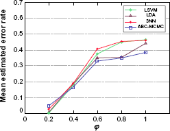
Expected classification error rates for fixed sample size n = 10 per class, fixed number of selected proteins d = 8, and varying coefficient of variation ϕ.

Effect of peptide efficiency factor

Finally, we investigate the impact of varying the peptide efficiency factor on the classification error rates. We do this by changing the lower bound in the range for e _i displayed in Table 1 from α = 0.1 to a value varying between 0 and 1. The peptide efficiency factor affects how many ions an instrument can detect for a given peptide. Larger values for e _i imply a smaller transmission loss for the corresponding peptide. Increasing the lower bound a will uniformly increase efficiency for all peptides, which corresponds to a better LC-MS instrument. We can see in Figure 5 that, indeed, the expected classification error rates tend to decrease with an increasing lower bound on the peptide efficiency factor, though somewhat modestly (all other things being equal). We can also observe that among all algorithms, the ABC-MCMC classification rule displays the smallest error rate over nearly the entire range in the plot.

Figure 5

Expected classification error rates for fixed sample size n = 10 per class, fixed number of selected proteins d = 8, and varying lower bound a for the peptide efficiency factor e _i ~ Unif(α, 1).

Conclusion

We proposed in this paper a model-based Bayesian approach for classification of LC-MS proteomics data with the ultimate goal of facilitating biomarker discovery for cancer research. Our approach combines state-of-the-art Bayesian computation techniques, namely, ABC and MCMC, for the calculation of the OBC. As expected, the proposed Bayesian classifier outperforms other approaches when sample size is small or the number of selected proteins to classify is large. We believe that our simulation using a subset of 4000 human protein drug targets and realistic parameter settings is indicative of the performance of the proposed methodology on real data. The challenges associated with designing experiments and obtaining appropriate real data to calibrate and validate the methodology go beyond the scope of the present paper and are intended to be part of future work.

Author Contributions

Conceived and designed the experiments: UB, UBN. Analyzed the data: UB. Wrote the first draft of the manuscript: UB. Contributed to the writing of the manuscript: UBN. Agree with manuscript results and conclusions: UB, UBN. Made critical revisions and approved final version: UB, UBN. Both authors reviewed and approved of the final manuscript.