Sage Journals: Discover world-class research

Abstract

Proteomics studies based on mass spectrometry (MS) are gaining popular applications in biomedical research for protein identification/quantification and biomarker discovery, especially for potential early diagnosis and prognosis of severe disease before the occurrence of symptoms. However, MS data collected using current technologies are very noisy and appropriate data preprocessing is critical for successful applications of MS-based approaches. Among various data preprocessing steps, peak alignment from multiple spectra based on detected peak sample locations presents special statistical challenges when effective experimental calibration is not feasible due to relatively large peak location variation. To avoid intensive tuning parameter optimization, we propose a simple novel Bayesian algorithm “random grafting-pruning Markov chain Monte Carlo (RGPMCMC)” that can be applied to global MS peak alignment and to follow certain modelbased sample classification criterion for using aligned peaks to classify spectrum samples. The usefulness of our approach is demonstrated through simulation study by making extensive comparison with other algorithms in the literature. Its application to an ovarian cancer MALDI-MS data set achieves a smaller 10-fold cross validation error rate than other current large scale methodologies.

Keywords

Mass spectrometry peak alignment random grafting-pruning Markov chain Monte Carlo (RGP CMC)reversible jump Markov chain Monte Carlo (RJMCMC)sample classification symmetric transition

1. Introduction

Genomics and proteomics technologies offer much promise in our understanding of fundamental biological processes by allowing us to simultaneously monitor the expression levels of tens of thousands of genes and proteins. Since proteins are the basic functioning units in the cells, there is a great interest to characterize individual molecular profiles based on proteomics for reliable biomarker discovery and effective disease diagnosis/prognosis/treatment. In proteomics research, mass spectrometry (MS) is the most widely used instrument to allow for the mass measurement of molecules, where a mass spectrometer determines chemical compounds’ molecular weight by ionizing, separating, and measuring molecular ions according to their mass-to-charge ratio (m/z: unit Da) and a mass spectrum is the standard data output for analysis and interpretation (Link et al. 1999), where the x-axis represents m/z value (Da) and the y-axis represents intensity (enrichment of particles with certain m/z). Recently, Yu et al. (2005) reviewed current approaches on the extraction of the most relevant information from the raw mass spectra to identify disease biomarkers. A standard MS data analysis usually involves background noise removal, smoothing, intensity normalization, peak identification and alignment, and biomarker identification. The false positive and false negative peaks may exist in taking local maxima as peaks (Coombes et al. 2003) and peak location variation may be due to differences in sample preparation, chemical noise, co-crystallization, deposition of the matrix-sample onto the target, and laser position on the target among others. Several statistical methods have been proposed to reduce the background noise (Coombes et al. 2003; Satten et al. 2004; Coombes et al. 2005a and Randolph and Yasui, 2006). Morris et al. (2005) applied translation-invariant wavelet transformations to the raw spectra and performed peak detection using the mean spectrum derived from a group of spectra, where they assumed calibration can be done in advance experimentally or by interpolation to make common peaks stay closely together, and only false negatives are possible. However, Coombes et al. (2005b) pointed out that, peak location variation, caused by a spread of initial particle velocities at the starting end of mass spectrometer tube, makes calibration more difficult. Compared to background noise removal, peak identification and alignment is more challenging and critical by providing the links of underlying peptides across all spectra. However, existing algorithms for peak alignment are mostly ad hoc and based on heuristic arguments (Nielsen et al. 1998; Johnson et al. 2003; Torgrip et al. 2003; Eilers, 2004; Tibshirani et al. 2004 and Randolph and Yasui 2006), where some parameters need to be optimized empirically and/or subjectively. In this paper, we work on the detected peak samples (possibly with associated intensities) coming from certain protocol. In view of hundreds of features (peaks) in each spectrum, due to complex chemical and physical mechanisms undergoing the mass spectrometry, throughout this paper, we assume that substantial individual peak location variation is existent, say up to one half of the interval between neighboring peaks, thus calibration may be in lack of power. Moreover, we consider statistically false positives and negatives to make our model more accountable. Overall, we will assume that each set of potential peak samples corresponding to the true peak follows an individual composite distribution regulated by true peak location, peak sample location variation, false positive and false negative rates. An effective simple Bayesian MCMC algorithm is proposed to do peak alignment (biomarker identification) and downstream sample classification, where all individual sets of parameters for each true potential peak are able to be estimated in a universal modeling framework without intensive tuning parameter optimization. Our algorithm is much computationally simpler than other available MCMC algorithms which could be applied to MS alignment while retaining competing performance.

The rest of this article is organized as follows: Section 2 introduces Bayesian dimension matching problem and proposes our simplified approach; Section 3 summarizes simulation results to demonstrate the efficiency and reliability of our algorithm; Section 4 illustrates the applications of our approach to a real MS data set; Section 5 considers joint analysis of peak alignment and sample classification; Section 6 concludes with discussions; and some technical details are given in the appendix.

2. Methods

2.1. Dimension-Matching Statistical Model

We now develop a simple novel MCMC algorithm, random grafting-pruning Markov chain Monte Carlo (RGPMCMC) which can be applied to MS peak alignment from mass charge ratio information. Within Bayesian framework, we are often interested in the posterior distribution of the dimension-varying parameter θ. The prior distribution π(θ)is represented as $\sum_{k \in N} π (θ_{K} | K) π(K)$ , where N is positive integer set and $π (θ_{k} | K)$ is the individual prior distribution within the K-dimensional space and π(K)is the mixture probability for dimension K. Since $π(K, θ_{k})= π(K)π(θ|K)$ , the posterior distribution of (K,θ_K)

\begin{array}{l} π (K, θ_{k} | X) = \\ \frac{f (X | θ_{k}) π (θ_{k}) (K)}{\sum_{K \in K} (\int_{Θ_{k}} f (X | θ_{k}) π (θ_{k}) d θ_{k}) π (K)}, \end{array}

(1)

where the denominator is the normalization constant not needed for posterior sampling. Change point model usually involves dimension-matching in two typical cases: one single ordered series where change points are taken as those separating successive discrete points, and multiple ordered series where change points correspond to physical locations in the continuous space. For the discrete case, the partitioning and wrapping up the segments leads to an exponentially increasing computational cost as the model space grows (Denison et al. 2002), and frequentist's approaches only either work on very few change points or special algorithms (Guan, 2004; Olshen and Venkatraman, 2004). Recently, Fearnhead (2005) proposed an exact non-MCMC sampler by recursive partition, and Loschi, Cruz and Arellano-Valle (2005) introduced the product partition model based Bayesian algorithm which stems from Yao (1984) and Barry and Hartigan (1992, 1993). For the continuous case, the readers are referred to sampling-based algorithms: the reversible jump MCMC (RJMCMC) by Green (1995), the birth-and-death process MCMC (BDMCMC) and continuous time process MCMC (CTMCMC) by Stephens (2000a, 2000b), Bayesian cluster detection in maps (Knorr-Held and Raßer, 2000) and others. Cappέ, Robert and Rydέn (2003) showed that, the acceptance probability of the usual MCMC methods is replaced by differential holding times in BDMCMC, and RJMCMC converges to a limiting continuous time birth-and-death process on an appropriate rescaling of time. They also demonstrated that, RJMCMC and CTMCMC have similar computational performance while the latter demands expensive death rate computation. Obviously, discretization is neither always suitable nor efficient for sophisticated change point identification in the continuous space. The present work introduces a simple MCMC algorithm in the context of multiple MS peak alignment by considering all uncertainties including peak number, peak locations, peak sample location variations, false negative and false positive rates. Neither the error-prone Jacobian terms in RJMCMC, the intensive death rate calculation in CTMCMC, nor the computationally expensive recursive partition in other algorithms is needed by our method.

Before starting with our statistical model, we assume local maxima (discrete locations) have been detected as peak samples for each raw mass spectrum. In MS peak alignment, peak sample location variation may linearly depend on m/z magnitude (Yasui et al. 2003), and log-transformation of m/z achieves peak sample location variation homogeneity, this observation will justify the identical prior specification for peak sample location variations across true peaks (details later). For notational simplicity, we use m/z instead of log (m/z) in the following discussions and assume that the m/z domain is [(m/z)_min, (m/z)_max]. The underlying K-dimensional true peak location vector is ${\tilde{S}}_{k}$ = (s₁, s₂, …, s_K), where the peak locations are generally separated by at least a distance threshold, say no less than d. The data to be analyzed from multiple spectra are the detected peak sample locations y_ij (j = 1, …, n_i, i = 1, …, I), where i is the index for spectra, j is the peak sample index within each spectrum (with increasing m/z), and n_i is the number of detected peak samples in the i-th spectrum. The peak samples are assumed to be normally distributed around their true peak s_k with standard deviation σ_k (k = 1, …, K) for locations. For the putative true peak set ${\tilde{S}}_{k}$ = (s₁, s₂, …, s_K), each detected peak sample j in i-th spectrum is assigned to its nearest putative true peak among ${\tilde{S}}_{k}$ , say n_y (i, j) (with possible multiple assignments to the same putative peak from a given spectrum). For certain true peak k, (1) when there is no peak sample assignment to it from a given spectrum, we consider it as a false negative case for this spectrum with probability fn_k; (2) when there are multiple peak sample assignments to it from a given spectrum, we consider it as a false positive case for this spectrum with probability fp_k; (3) otherwise we consider it as a non-false positive or negative case for this spectrum with probability 1 – fn_k – fp_k. Our prior hypothesis is that, each true peak shows these three types of cases proportionally under the homogeneity assumption for the spectra and identical peak sample detection protocol for each local m/z region, say for each true peak, on average 90% spectra will contribute single peak sample, 5% will contribute multiple peak samples and 5% will contribute no peak sample to the putative true peak. For these three cases, we assume an independent trinomial distribution Tri(I; fn_k, fp_k, 1 – fn_k – fp_k) for each true peak k in the context of numbers of grabbed peak samples from I spectra. Now we restate the following notations for model set-up: Y stands for the peak sample locations for all I spectra, which need not be a I-row matrix since the numbers of peak samples are not necessarily equal because of false negatives and/or false positives; ${\tilde{S}}_{k}$ is a K-dimensional vector of putative true peak locations (m/z's); ${\tilde{σ}}_{k}$ is a K-dimensional vector of peak sample location variations at putative true peaks; $\tilde{f} n_{k}$ and $\tilde{f} p_{k}$ are K-dimensional vectors of false negative and false positive rates at putative true peaks; n_y (i, j) is putative true peak assignment to peak sample j in the i-th spectrum; n_fn,k is the number of spectra without peak samples assigned to putative true peak k; n_fp,k is the number of spectra with multiple peak samples assigned to putative true peak k, and $n_{\bar{f n p, k}}$ is the number of spectra with single peak sample assigned to putative true peak k (Figure 1). The likelihood for the observed peak samples across all spectra is

Figure 1

Mass Spectrum Biomarker Model. (The left column is spectrum index, the vertical lines are putative true peaks, the horizontal circle lines are peak samples of each spectrum. The lower left dash rectangle represents a false negative case and the upper right dash rectangle represents a false positive case.)

\begin{matrix} f (Y | K, {\tilde{S}}_{K}, {\tilde{σ}}_{K}, \tilde{f} n_{K}, \tilde{f} n_{K}, \tilde{f} p_{K}) \\ = Π_{i = 1}^{I} \underset{1 \leq j \leq n_{j}}{Π} ϕ (y_{i j} | s_{n_{y} (i, j)}, σ_{n_{y} (i, j)}) \\ \times Π_{k = 1}^{K} f n_{k}^{n_{f n, k}} f p_{k}^{n_{f p, k}} {(1 - f n_{k} - f p_{k})}^{n_{\bar{n f n p, k}}} . \end{matrix}

(2)

We now describe the motivation for such a likelihood function which is crucial for Bayesian inference. The matching by minimum distance $(s_{n_{y} (i, j)})$ is to capture important clustering information. We believe that, this objective construction is reasonable compared to some alternatives, e.g. non-model based clustering algorithms, or piecewise binning method where each bin is assumed to hold exactly those peak samples for the individual putative true peak. The other part incorporating false positives and false negatives is mainly a technical statistical consideration, since it is very hard to accurately claim which peak sample is a true false positive or false negative. To sum up, in spite of substantial measurement errors underlying high-throughput mass spectra, we pursue a reasonable eclectic theme to tackle biomarker profile estimation. For notational convenience, “peak” represents putative true peak for the biomarker profile hereafter, other than detected peak sample from each spectrum. On the prior part, we assume that K follows a truncated Poisson or discrete uniform distribution on {K_min, …, K_max}. As Green (1995) suggested, the peak locations are taken as even-numbered order statistics from 2K + 1 points uniformly distributed on an L-length interval [(m/z)_min, (m/z)_max] (for convenience, s₀ = (m/z)_min, s_K+1 = (m/z)_max) to avoid too many short steps, which has density $Π_{k = 1}^{K + 1} (s_{k} - s_{k - 1}) / L^{2 K + 1}$ as suggested by Green (1995). To make use of conjugate prior, π(σ²) is taken as Inverse-Gamma (ν,η) density $(σ^{2}) -^{(v + 1)} e^{- 1 / (σ^{2} η)} η^{- v} / Γ (v);$ the joint prior distribution for (fn, fp, – fn – fp) is a 3-dimensional Dirichlet distribution with density $D (f n, f p, 1 - f n - f p | α_{1}, α_{2}, α_{3}) = {(f n)}^{α_{1} - 1} {(f p)}^{α_{2} - 1} (1 - f n - 2) f p)^{α_{3} - 1} Γ (α_{1}) Γ (α_{2}) Γ (α_{3}) / Γ (α_{1} + α_{2} + α_{3})$ . The posterior distribution is

\begin{matrix} f (K, {\bar{S}}_{k}, {\tilde{σ}}_{K}, f n_{K}, f p_{K} | Y) Π_{i = 1}^{I} Π_{1 \leq j \leq n_{j}} ϕ (y_{i j}; s_{n_{y} (i, j)}, σ_{n_{y} (i, j)}) & (Normal Dist .) \\ \times Π_{k = 1}^{K} f n_{k}^{n_{f n, k}} {(1 - f n_{k} - f p_{k})}^{n_{\bar{f n p, k}}} & (trinomial Dist .) \\ \times π (K, S_{k}) Π_{k = 1}^{K} [D (f n_{k}, f p_{k}, 1 - f n_{k} - f p_{k} | α_{1}, α_{2}, α_{3}) \times Π_{k = 1}^{K} I G (σ_{k}^{2} | v, η)] & (prior Dist .) \end{matrix}

(3)

2.2. Random Grafting-Pruning Markov Chain Monte Carlo(Rgpmcmc)

Motivated by Green (1995), our algorithm is based on a redesigned universal “naively informative” parameter proposal involving peaks and the other parameters concurrently without the need for Jacobian terms. We also propose four move types (+, –, H, S), where “+” means peak birth proposal, “–” means peak death proposal, “H” means parameter (σ², fn and fp) proposal excluding peaks and “S” means peak location mutation with peak number unchanged. We specify (+, –, H, S) probabilities as $(π (+), π (-), π (H), π (S))$ .

Parameter Sampling Process

1)
First we choose one of these four move types based on move type probabilities (π(+), π(–), π(H), π(S)), where π(+) = π(–).
2)
For the “+” move type, we describe the parameter proposal process: If K_old = K_max, we go to 1) since the upper threshold is reached; if K_old < K_max, we randomly sample one of the K_old + 1 intervals formed by current K_old peaks, say (s_j, s_j+1), with equal probability 1/(K_old + 1). We may assign j + 1 to this new peak index ^* and the following indexes increase by one accordingly. Within this sampled interval, we propose ( $(s_{}, σ_{}^{2}, f n_{}$ and fp_) for peak candidate ^* as follows:
i.
True peak location proposal for peak birth:
$s_{} = g_{s_{}} (U_{1}; s_{j}, s_{j + 1}) \in (s_{j}, s_{j + 1}),$

where g_s(U₁; s_j, s_j+1) is a one-to-one mapping from random variable U₁ to peak location s_ given s_j and s_j+1. We take $g_{σ_{}^{2}} (U_{2}; σ_{j}^{2}, σ_{j + 1}^{2})$ to be $(s_{j} + s_{j + 1} g_{1} (U_{1})) / (1 + g_{1} (U_{1}^{})),$ or $(s_{} - s_{j}) / (s_{j + 1} - s_{}) = g_{1} (U_{1})$ , where g₁(·) is any monotonic function with domain [0, 1] and range [0, ∞), and U₁ ~ U [0, 1]. It can be seen that, s_* is a monotonically increasing function of U₁. We simply use g₁(u) = u/(1 – u), thus s_* = s_j + (s_j+1 – s_j) U₁, a uniform random variable ∊ (s_j, s_j+1).
ii.
Peak sample location variance proposal for peak birth:
$σ_{}^{2} = g_{σ_{}^{2}} (U_{2}; σ_{j}^{2}, σ_{j + 1}^{2}),$

where $g_{σ_{}^{2}} (U_{2}; σ_{j}^{2}, σ_{j + 1}^{2})$ is a one-to-one mapping from random variable U₂ to peak sample location variance $g_{}^{2}$ given $σ_{j}^{2}$ and $σ_{j + 1}^{2}$ . We take $g_{σ_{}^{2}} (U_{2}; σ_{j}^{2}, σ_{j + 1}^{2})$ to be ${(σ_{j}^{2} σ_{j + 1}^{2})}^{1 / 2} g_{2} (U_{2})$ or $(σ_{} / σ_{j}) / (σ_{j + 1} / σ_{}) = g_{2} (U_{2})$ , where g₂(·) is any monotonic function with domain [0, 1] and range [0, ∞), and U₂ ~ U [0, 1]. It can be seen that, $σ_{2}^{}$ is a monotonically increasing function of U₂. We simply use g₂(u) = u/(1 – u), thus $σ_{}^{2} = {(σ_{j}^{2} σ_{j + 1}^{2})}^{1 / 2} U_{2} / (1 - U_{2})$ .
iii.
Peak sample false negative and false positive rate proposal for peak birth:
$(f n_{}, f p_{}) = {\tilde{g}}_{f n_{}, f p_{}} (U_{3}, U_{4}; f n_{j}, f p_{j}, f n_{j + 1}, f p_{j + 1}),$

where ${\tilde{g}}_{f n_{}, f p_{}} (U_{3}, U_{4}; f n_{j}, f p_{j}, f n_{j + 1}, f p_{j + 1})$ , is a one-to-one mapping from (U₃, U₄) to (fn_,fp_) given (fn_j, fp_j) and (fn_j+1, fp_j+1). Specifically, for peak ^, we use O^* to represent “false negative or positive” odds and R_* to represent “false negative vs. positive” ratio, i.e.
$O_{} = (f n_{} + f p_{}) / (1 - f n_{} - f p_{}) and R_{} = f n_{} / f p_{},$
(4)

the false negative and false positive rate proposal is realized in two sequential steps:
1)
O_* proposal:
$O_{} = {(O_{j} O_{j + 1})}^{1 / 2} g_{3} (U_{3}),$
(5)

i.e. (O_/O)^1/2/(O_j+1/O_)^1/2 = g₃(U₃), where g₃(·) is any monotonic function with domain [0, 1] and range [0, ∞), and U₃ ~U[0, 1]. It can be seen that, O^ is a monotonically increasing function of U₃, we simply use g₃(u) = u/(1 – u).
2)
R_* proposal:
$R_{} = {(R_{j} R_{j + 1})}^{1 / 2} g_{4} (U_{4}),$
(6)

i.e. (R_/R_j)^1/2/(R_j+1/R_)^1/2 = g₄(U₄), where g₄(·) is any monotonic function with domain [0, 1] and range [0, ∞), and U₄ ~ U[0, 1]. It can be seen that, R_ is a monotonically increasing function of U₄, we simply use g₄(u) = u/(1 –u).

Note that the constraint 0 ≤ fn_* + fp_* ≤ 1 holds under this proposal. The ${\tilde{g}}_{f n_{}, f p_{}} (U_{3}, U_{4}; f n_{j}, f p_{j}, f n_{j + 1}, f p_{j + 1})$ function is a combination of O_* proposal and R_* proposal in this case. fn_* and fp_* are jointly proposed to meet the constraint. The Jacobian of transforming (fn_j,fp_j,fn_j+1,fp_j+1,u₃, u₄) into ((fn_j,fp_j,fn_,fp^,fn_j+1,fp_j+1) is calculated by chain rule (see appendix).

When the insertion of the peak birth candidate is before the first peak or after the last peak, there are no real double neighbors. In this case, we take the duplicates of peak birth candidate's unique succeeding or preceding neighbor as two virtual neighbors for proposal implementation. In this move type, we realize the sequential uniform lift for fn_+fp_ and subsequent conditional uniform lift for fn_* within fn_* + fp_. We claim that, the peak birth proposal by “+” move type, along with the peak death proposal by the following “–” move type, constructs a symmetric transition, i.e. equally probable events (Proposition 3). So the acceptance probability in the Metropolis-Hastings algorithm within Gibbs sampler is simply
$\min {1, \frac{f (K, {\tilde{S}}_{K}, {\tilde{σ}}_{K}, \tilde{f} n_{K}, \tilde{f} p_{K} [after peak death proposal] | Y)}{f (K, {\tilde{S}}_{K}, {\tilde{σ}}_{K}, \tilde{f} n_{K}, \tilde{f} p_{K} [after peak death proposal] | Y))}} .$

3)
For the “–” move type, the parameter proposal process is: If K_old* = K_mim we go to 1) since the lower threshold is reached; if K_old > K_mim we randomly sample one from current K_old peaks with equal probability 1/K_old, say index ^, to delete. Then we simply abandon the associated $s_{}, σ_{}^{2}, f n_{}$ and $f p_{}$ for likelihood reconstruction. The acceptance probability in the Metropolis-Hastings algorithm within Gibbs sampler is simply
$\min {1, \frac{f (K, {\tilde{S}}_{K}, {\tilde{σ}}_{K}, \tilde{f} n_{K}, \tilde{f} p_{K} [after peak death proposal] | Y)}{f (K, {\tilde{S}}_{K}, {\tilde{σ}}_{K}, \tilde{f} n_{K}, \tilde{f} p_{K} [after peak death proposal] | Y))}} .$

The “+/–” move type is demonstrated in Figure 2 for only peak location model.
Figure 2
Symmetric Transition for Peak Birth/death Proposal. (Each rectangle represents a uniform peak birth proposal domain, each internal vertical boundary represents a possible peak death proposal location.)

4)
For the “S” move type, the parameter proposal process is: We randomly sample one of current peaks, say ^, with equal probability 1/K_old, and take the two neighboring peak intervals which peak ^* separates as a fused interval. A peak location is uniformly randomly drawn within this fused interval for a new candidate peak to replace s_. The other parameters associated with this peak location mutation is kept unchanged, or they could be changed as a set within the uniformity framework. This is also a symmetric transition (Proposition 2). So the acceptance probability in the Metropolis-Hastings algorithm within Gibbs sampler is simply
$\min {1, \frac{f (K, {\tilde{S}}_{K}, {\tilde{σ}}_{K}, \tilde{f} n_{K}, \tilde{f} p_{K} [after peak mutation proposal] | Y)}{f (K, {\tilde{S}}_{K}, {\tilde{σ}}_{K}, \tilde{f} n_{K}, \tilde{f} p_{K} [after peak mutation proposal] | Y))}} .$

5)
For the “H” move type, the posterior distribution of each $σ_{k}^{2}$ is Inverse-Gamma (ν′, η′), where $v' = v + (\sum_{y i j_{2} \in p e a k K} 1) / 2, η' = 1(1/η+ \sum_{y i j \in p e a k k} {(y_{i j} - s_{k})}^{2} / 2)$ . The joint posterior distribution of each (fn_k,fn_k, 1 – fn_k* – fp_k) is Dirichlet $(α_{1} + n_{f n, k}, α_{2} + n_{f p, k}, α_{3} + n_{\bar{f n p,_{k}}})$ . We sample the whole set of these parameters once.

Remark: This algorithm is a random scan (by move type probabilities) version of Gibbs sampler introduced by Gelfand and Smith (1990) with generalized parameter components:
1)
peak (described by location, peak sample location variance, false negative and positive rates) birth or death changes the number of parameter sets by move type “+” or “–” in the aforementioned parameter sampling proposal;
2)
peak location mutation does not change the number of parameter sets by move type “S” in the aforementioned parameter sampling proposal;
3)
peak sample location variance or false negative/positive rate sampling does not change the number of parameter sets by move type “H” in the aforementioned parameter sampling proposal.

The associated propositions and the detailed description of RGPMCMC are given in the appendix. The following proposition justifies the correct convergence.

Proposition: The induced Markov chain is irreducible, aperiodic, and ergodic.

Interpretation: In view of independent uniform proposals for non-peak parameter set and diverse move types, given any arbitrarily small neighborhood of a current state there is a positive probability that the chain lies in that neighborhood after one sampling iteration, thus the aperiodicity is verified; the irreducibility is established since the chain can move from any state to any other state one step at a time.
3. Simulation Study

In this section, we study the RGPMCMC performance under diverse circumstances and make comparison with other approaches in the literature.

3.1. Prior Sensitivity Analysis for Rgpmcmc

We consider different priors and study the discrepancy between the specified true peak locations and the estimated peak locations. Compaq Fortran 90 is our development package and we use IMSL Fortran Numerical Library to generate random numbers. 200 spectra are simulated for each of the six simulations, the set-ups and priors are listed in Table 1, where four true peaks are considered, the peak location vectors specify the true peak locations, the σ vectors specify the peak sample location variations at true peaks, the fn and fp vectors jointly specify the probabilities for us to simulate no peak sample (with probability fn), multiple peak samples (with probability fp), or single peak sample (with probability 1 – fn – fp) for each true peak from individual spectrum. The Inverse-Gamma and Dirichlet priors are for peak sample location variances and false negative and positive rates at putative true peaks. The peak number prior is K ~ U [1, 20], the starting peak number is 11, and move type probabilities are: π(+) = 0.45, π(–) = 0.45, π(H) = 0.05, and π(S) = 0.05. With burn-in 10,000 and thinning 1,000, each collection of 1,000 posterior samples takes several minutes on a PC powered by Celeron CPU. The results are given in Figure 3. In simulation 1, the true peaks are clearly clustered and the peak estimation is good. In simulation 2 with larger peak sample location variations and false positive/negative rates, the same number of peaks are identified as the true peak number under highly informative priors. By modifying peak sample location variation priors, we observe that, under large true variations, the peak estimation under less informative variation priors is worse than that under more informative variation priors. More uncertainties are introduced in simulation 3, and fewer peaks are identified than the true peak number. By modifying peak sample location variation priors, we observe that, when the variation priors are consistent with the true variation in terms of mean value, the peak number estimation seems to be better than inconsistent variation priors. Simulation 4 shows that, the informative peak sample location variation priors may lead to good estimation even when the peaks’ associated parameters are different, so does simulation 5, where unevenly distributed peaks are considered. In simulation 6, even when the parameter priors become much less informative, the peak estimation performs well, since the true peaks are sharply surrounded by corresponding peak samples. These observations show that, informative a priori knowledge is desirable for reliable estimation.

Table 1
Simulation Configurations (IG: Inverse-Gamma prior for σ², D: Dirichlet prior for (fn, fp,1 – fn – fp)).

Peak location (s₁, s₂, s₃, s₄) = (1/5, 2/5, 3/5, 4/5)

(1) σ 0.05 0.05 0.05 0.05 (2) σ 0.10 0.10 0.10 0.10

fn 0.10 0.10 0.10 0.10 fn 0.20 0.20 0.20 0.20

fp 0.10 0.10 0.10 0.10 fp 0.20 0.20 0.20 0.20

IG(5, 100), D(1, 1, 8) IG(26, 4), D(40, 40, 120)

(3) σ 0.20 0.20 0.20 0.20 (4) σ 0.02 0.08 0.08 0.02

fn 0.30 0.30 0.30 0.30 fn 0.10 0.20 0.30 0.40

fp 0.40 0.40 0.40 0.40 fp 0.10 0.20 0.30 0.40

IG(6, 5), D(5, 5, 5) IG(20, 6), D(5, 5, 10)

Peak location (s₁, s₂, s₃, s₄) = (1/16, 3/16, 7/16, 15/16)

(5) σ 0.02 0.08 0.08 0.02 (6) σ 0.02 0.02 0.02 0.02

fn 0.10 0.20 0.30 0.40 fn 0.10 0.10 0.10 0.10

fp 0.10 0.20 0.30 0.40 fp 0.10 0.10 0.10 0.10

IG(20, 6), D(5, 5, 10) IG(3, 2), D(2, 2, 2)

Figure 3

Simulations and Estimations (The simulation directly produces the peak samples for 200 patients which are plotted in each odd row of panels without the need for peak sample detection by data preprocessing, the y-axis is patient index and the x-axis is log(m/z). The alignments are compared by gridded walls given in each even row of panels. From top to bottom: true peaks, aligned peaks by RGPMCMC, aligned peaks by RJMCMC, aligned peaks by scale-space approach, aligned peaks by super-set approach and aligned peaks by PAM clustering algorithm.)

3.2. Comparison with Some Non-Mcmc approaches

We first make comparisons with other non-MCMC algorithms represented by the recently developed scale-space approach (Yu et al. 2006a), super-set approach (Yu et al. 2006b), and Partitioning around Medoids (PAM) approach (Kaufman and Rousseeuw, 1990). For the six simulations in Section 3.1, the combined peak sample locations from 200 spectra along with the optimal cluster number minimizing the “median split silhouette” (Pollard and van der Laan, 2002) are taken as PAM inputs, S-plus function pam offers the medoid (cluster center) locations. These results are also included in Figure 3. Overall, RGPMCMC performs better than non-MCMC methods; the scale-space result is little better than the super-set result in terms of robustness; the PAM algorithm is not specifically designed for peak alignment, so it may perform poorly under certain circumstances, say simulations 2 and 3, where RGPMCMC can not recover all true peaks either.

3.3. Comparison with Reversible Jump Markov Chain Monte Carlo

We apply the same simulated data in Section 3.1 and make comparison with reversible jump Markov chain Monte Carlo (RJMCMC) algorithm by Green (1995). RGPMCMC and RJMCMC differ in the method for proposing move type “+” and/or “–” (peak birth and/or death), where the former conditions on the active Markov chain by making use of equally probable peak birth and death proposals, while the latter makes use of additional variables to construct a one-to-one matching for dimension changing (details are given in the appendix). The same prior specifications for RGPMCMC in Section 3.1 are applied to RJMCMC. We consider two starting peak numbers, 11 and 1, both equally partitions the m/z range.

Initial Peak Number = 11

1)
Figure 3 also compares the alignments by RGPMCMC and RJMCMC, where no difference between RGPMCMC and RJMCMC exists.
2)
The peak number iteration comparison is given in Figure 4, where the burn-in = thinning = 1,000. The third row of dual panels pinpoint 3 or 4 peaks, the 4:3 ratios are 0.124 and 0.122 for RGPMCMC and RJMCMC respectively, which is close to each other. The acceptance rate for peak birth and/or death proposals should be almost identical for these two algorithms.
Figure 4
Peak Number Sampling Series by RGPMCMC and RJMCMC from Simulation Study (burn in = thinning = 1,000, the initial peak number = 11.)

3)
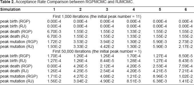
The peak number iteration comparison before reaching reasonable peak number (1,000th iteration) can be seen from Figure 5. For these six simulations, peak birth and/or death, and peak mutation acceptance rates are compared in Table 2, which are close to each other.
Figure 5
Peak Number Sampling Series by RGPMCMC and RJMCMC from Simulation Study (first 1,000 iterations with initial peak number 11)

4)
The reasonable peak number is reached after almost the same number of iterations (~1,000) by GPMCMC and RJMCMC, which have similar efficiency for peak number identification.

Table 2.
Acceptance Rate Comparison between RGPMCMC and RJMCMC.

Simulation 1 2 3 4 5 6

First 1,000 iterations (the initial peak number = 11)

peak birth (RGP) 0.00E-4 0.00E-4 0.00E-4 0.00E-4 0.00E-4 0.00E-4

peak birth (RJ) 0.00E-4 0.00E-4 0.00E-4 0.00E-4 0.00E-4 0.00E-4

peak death (RGP) 6.70E-3 1.55E-2 1.55E-2 1.33E-2 1.55E-2 1.55E-2

peak death (RJ) 6.70E-3 1.55E-2 1.55E-2 1.33E-2 1.55E-2 1.55E-2

peak mutation (RGP) 1.72E-2 3.53E-2 3.94E-2 1.30E-2 5.90E-3 2.73E-2

peak mutation (RJ) 1.93E-2 3.33E-2 4.42E-2 1.30E-2 5.90E-3 2.17E-2

First 50,000 iterations (the initial peak number = 1)

peak birth (RGP) 1.70E-4 1.26E-4 1.26E-4 1.70E-4 1.27E-4 8.50E-5

peak birth (RJ) 1.27E-4 1.26E-4 8.44E-5 1.28E-4 1.27E-4 8.43E-5

peak death (RGP) 0.00E-4 4.26E-5 2.12E-4 4.20E-5 2.53E-4 7.59E-4

peak death (RJ) 1.26E-4 4.25E-5 2.54E-4 4.20E-5 4.21E-5 7.21E-4

peak mutation (RGP) 1.71E-2 4.27E-2 4.08E-2 1.21E-2 8.96E-3 1.02E-2

peak mutation (RJ) 1.56E-2 3.04E-2 4.90E-2 8.51E-3 6.38E-3 1.41E-2

Initial Peak Number = 1
1)
The peak number iteration comparison is given in Figure 6, where the burn-in = thinning = 1,000. The third row of dual panels pinpoint 3 or 4 peaks, the 4:3 ratios are 0.131 and 0.079 for RGPMCMC and RJMCMC respectively, where the ratio by RGPMCMC (0.131) is very close to peak number 11 case (0.124). Except for simulation 5, both RGPMCMC and RJMCMC identify the same number of peaks. For simulation 6, they all identify 3 peaks other than the true 4 peaks.
Figure 6
Peak Number Sampling Series by RGPMCMC and RJMCMC from Simulation Study (burn in = thining = 1,000 the initial peak number = 1.)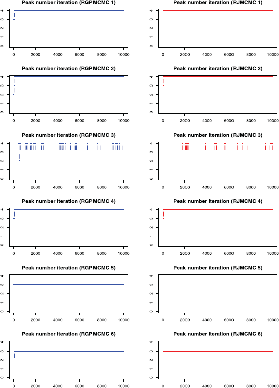

2)
The peak number iteration comparison before 50,000th iteration can be seen from Figure 7. For these six simulations, peak birth and/or death, and peak mutation acceptance rates are also compared in Table 2. The rates are still close to each other.

Figure 7
Peak Number Sampling Series by RGPMCMC and RJMCMC from Simulation Study (first 50,000 interations with initial peak number 1)

We find that, starting from a relatively large peak number is more capable of identifying true peaks by RGPMCMC and RJMCMC.
3.4. Mimic-ms Simulation Study

Simulation	1	2	3	4	5	6
First 1,000 iterations (the initial peak number = 11)
peak birth (RGP)	0.00E-4	0.00E-4	0.00E-4	0.00E-4	0.00E-4	0.00E-4
peak birth (RJ)	0.00E-4	0.00E-4	0.00E-4	0.00E-4	0.00E-4	0.00E-4
peak death (RGP)	6.70E-3	1.55E-2	1.55E-2	1.33E-2	1.55E-2	1.55E-2
peak death (RJ)	6.70E-3	1.55E-2	1.55E-2	1.33E-2	1.55E-2	1.55E-2
peak mutation (RGP)	1.72E-2	3.53E-2	3.94E-2	1.30E-2	5.90E-3	2.73E-2
peak mutation (RJ)	1.93E-2	3.33E-2	4.42E-2	1.30E-2	5.90E-3	2.17E-2
First 50,000 iterations (the initial peak number = 1)
peak birth (RGP)	1.70E-4	1.26E-4	1.26E-4	1.70E-4	1.27E-4	8.50E-5
peak birth (RJ)	1.27E-4	1.26E-4	8.44E-5	1.28E-4	1.27E-4	8.43E-5
peak death (RGP)	0.00E-4	4.26E-5	2.12E-4	4.20E-5	2.53E-4	7.59E-4
peak death (RJ)	1.26E-4	4.25E-5	2.54E-4	4.20E-5	4.21E-5	7.21E-4
peak mutation (RGP)	1.71E-2	4.27E-2	4.08E-2	1.21E-2	8.96E-3	1.02E-2
peak mutation (RJ)	1.56E-2	3.04E-2	4.90E-2	8.51E-3	6.38E-3	1.41E-2

We mimic the mass spectra using the R package developed by Coombes et al. (2005b), where wide-ranging factors are considered to create the uncertainty, including the acquisition time resolution of the detector, the distribution of initial particle velocities, isotope distribution and others. Ideally, our six simulated mass spectrum groups have 5, 10, 20, 40, 80 and 160 peaks without incorporating any uncertainty and the R simulator produces six mean spectra, where the particles with large mass value (>20,000 Da) have broader hills due to more isotopes (Figure 8). Each mean spectrum leads to 100 uncertainty involved random replicative spectra subject to peak sample detection. For them we smooth spectrum with a predefined Gaussian function (window size of 15), search local maxima in the local neighborhood of 15 data points as peak samples, the minimal intensity value of peaks should be not smaller than 100. The RGPMCMC pinpoints 5, 9, 18, 35, 62 and 112 peaks (Inverse-Gamma (6,500) is peak sample location variance prior, Dirichlet (5,5,90) is false negative and positive rate prior, the starting peak numbers are 10, 20, 40, 80, 160 and 320); the clustering method in Tibshirani et al. (2004) pinpoints 5, 9, 19, 36, 69 and 174 peaks (the tuning parameters are selected as suggested in Tibshirani et al. (2004)). The alignment comparison is also given in Figure 8, where the clustering method tends to identify redundant peaks at large masses (the arrows in the bottom panels of Figure 8), while RGPMCMC performs better in this region; both methods identify less peaks in certain dense regions (bottom panels in Figure 8), while RGPMCMC sometimes combine too concentrated peaks into one peak (the arrows in the middle panels of Figure 8). Overall, these two approaches have similar performance in this simulation scenario.

Figure 8

Mimic-MS Simulations and Estimations (The R simulator produces the spectrum profiles given in each odd row of panels, 100 random spectra were simulated for each of them for peak sample detection. The y-axis is intensity and the x-axis is m/z. After peak sample detection by data preprocessing, the alignments are compared by gridded walls given in each even row of panels. From top to bottom: true peaks, aligned peaks by RGPMCMC and aligned peaks by clustering algorithm.)

4. Application to Real Data

We model the same ovarian cancer data source as used by Wu et al. (2003) (available on-line at http://bioinformatics.med.yale.edu/MSDATA), where the healthy group has 77 patients and the cancer group has 93 patients. The individual spectrum has tens of thousands of (m/z, intensity) pairs and looks like a more complicated and error-involving version of those simulated profiles in Section 3.4 (Figure 8). The data preprocessing on original spectra involves baseline subtraction, smoothing, intensity normalization and peak sample detection by local maxima as described in Section 3.4. The median of the original peak sample numbers after pre-processing is 249 for the healthy group and 241 for the cancer group. The values of log(m/z) range from 6.565 to 8.200. We use move type probabilities (π(+) = 0.45, π(–) = 0.45, π(H) = 0.05, π(S) = 0.05) and the interval constraint d = 10^–5. If this constraint is not met at one iteration, we simply resample the parameters. Richardson and Green (1997) observed that, proper posterior distributions may be not possible under fully noninformative priors, so we apply (α₁ = 5, α₂ = 5, α₃ = 90) to Dirichlet priors, and (ν = 3, η = 2⁶) to Inverse-Gamma priors. Different peak number priors, either truncated Poisson [100, 600|λ] or Uniform [100, 600] lead to similar results. The starting peak number is K = (K_min + K_max)/2, the initial peak locations are equal K-partition of log(m/z) range, burn-in is 10,000, and thinning is 1,000. We recommend to start with a relatively large peak number. The sampler approaches the reasonable peak number very quickly and usually sticks around and mostly does effective single peak mutations once approaching the true peak number. Occasional peak number jump ups are highly efficient for joint peak number and location estimation. The alignment results are given in Figure 9. The sampling series of peak number are given in Figure 10, where we empirically identify the modes of the posterior peak number distribution as 274 (healthy group) and 260 (cancer group). The false negative rate and false positive rate estimations are given in Figure 11 with a significant negative correlation. The posterior peak sample location variation medians are given in Figure 12, where the inconsistency of the first point possibly arises from edge effect, so do false negative and positive rate median plots (Figure 11). The average peak distance (~(8.200 – 6.565)/290 = 0.0058) dominates the estimated peak sample location variation (~0.001). The sampler takes several thousand iterations to approach the reasonable peak number, thus an adaptive strategy with varying move type probabilities may be more efficient than the brute birth/death dominating proposal after that time point. The collection of the posterior samples in Figure 10 takes several days on a PC powered by Celeron CPU.

Figure 9

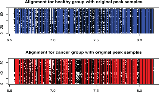
Aligned Peaks with Peak Sample Background (y-axis: patient index, x-axis: log(m/z). The vertical lines represent aligned peaks (biomarker profile) for each group, the dots in the background are the deteced peak samples for all patients by data preprocessing.)

Figure 10

Sampling Series of Peak Number (y-axis: peak number, x-axis: iteration index. The healthy group seems to have more peaks than cancer group.)

Figure 11

False Negative Rate and False Positive Rate Estimation (The left panel of first row is the histogram of false negatives at aligned peaks from healthy group, the right panel of first row is the histogram of false negatives at aligned peaks from cancer group; the left panel of second row shows the false negative medians at aligned peaks (represented by log(m/z)) from healthy group, the right panel of second row shows the false negative medians at aligned peaks (represented by log (m/z)) from cancer group; the next two rows are for false positives; the bottom row of panels show (false positive rate [x-axis], false negative rate [y-axis]) at aligned peaks for healthy group and cancer group.)

Figure 12

Posterior Medians of Peak Sample Location Variation (The upper left panel is the histogram of peak sample location variation medians from healthy group, the upper right panel is the histogram of peak sample location variation medians from cancer group; the lower left panel shows peak sample location variation medians (healthy group) at aligned peaks represented by log (m/z), the lower right panel shows peak sample location variation medians (cancer group) at aligned peaks represented by log(m/z).)

5. Sample Classification

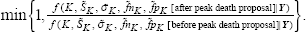
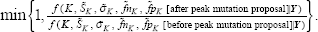
Effective sample classification is as important as biomarker profile estimation. Wu et al. (2003) compared a number of sample classification methods without cross-validation and Tibshirani et al. (2004) reached error rates no less than 35%. Since the peak number is biologically variable between healthy and cancer groups, the current equal-peak-number based classifications may not be very suitable. Without considering cross-validation, we simply calculate the two log-likelihood functions for each preprocessed spectrum given fitted model (healthy group or cancer group) from Section 4, where the estimated parameters are taken from posterior medians. The histograms of log-likelihoods of all spectra from both healthy group and cancer group along with the log-likelihood difference histograms are given in Figure 13. From the log-likelihood difference empirical distributions in the bottom panels of Figure 13, we simply take the proportions of negative values as type I error rates: 28.6% for testing: Healthy vs. Cancer and 10.8% for testing: Cancer vs. Healthy, which are overly optimistic. Denote ỹ = (y₁, y₂, …, y_N) as the spectrum peak sample location vector to be classified, ${\tilde{s}}_{H} = (s h_{1}, s h_{2}, …, s h_{K_{H}})$ is the estimated true peak location vector for the healthy population, and ${\tilde{s}}_{C} = (s c_{1}, s c_{2}, …, s c_{K_{c}})$ is the estimated true peak location vector for the cancer population (usually K_H ≠ K_C). We propose a minimum ${\bar{L}}_{1}$ distance sample classification rule. For each sh_k (1 ≤ k ≤ K_H), we identify its nearest neighbor yn_kk from ỹ and form a L₁ distance summand |sh_k – yn_kk|, the same rule applies to each sc_k (1 ≤ k ≤ K_C). To be conservative, we only use those deviations less than 0.003 (~half of the average peak interval) followed by arithmetic average over these selected estimated true peaks. The ${\bar{L}}_{1}$ distances between the new spectrum ỹ from healthy population and cancer population are

{\bar{L}}_{1} (\tilde{y}, H) = \frac{1}{K'_{H}} \sum_{k = 1}^{K_{H}} 1_{s e l e c t e d} | s h_{k} - y_{n_{h k}} |

and

{\bar{L}}_{1} (\tilde{y}, C) = \frac{1}{K'_{C}} \sum_{k = 1}^{K_{C}} 1_{s e l e c t e d} | s c_{k} - y_{n_{c k}} |,

where $K_{H}^{'}$ is the number of selected true peaks from ỹ_H based on 0.003 threshold, and $K_{C}^{'}$ is the number of selected true peaks from ỹ_C, 1_selected is the indicator function of selection. The class leading to smaller ${\bar{L}}_{1}$ would be predicted. Our 10 fold cross-validation is implemented as follows: we equally divide both the healthy and the cancer groups into ten disjoint pairs of testing set (H_i,C_i), (i = 1, …, 10). For each of these pairs, we combine the complementary nine sets as the corresponding healthy and cancer group training sets $(H_{i}^{'}, C_{i}^{'}), (i = 1, …, 10)$ , i.e. $H_{i}^{'} = U_{1 \leq k \leq 10, k \neq i} H_{k}$ and $C_{i}^{'} = U_{1 \leq k \leq 10, k \neq i} C_{k}$ . The exact 10 fold cross-validation would be done for each of these testing pairs (H_i, C_i) from fitting $(H_{i}^{'}, C_{i}^{'}), (i = 1, …, 10)$ . The results are given in Table 3. The type I error rate for hypothesis test: H₀: Healthy vs. H₁: Cancer is around 38.97%, and the type I error rate for hypothesis test: H₀: Cancer vs. H₁: Healthy is around 27.96%, and the overall sample misclassification rate from 10 fold cross-validation is around 32.94%. Our strict 10-fold cross validation error rate is less than that of Tibshirani et al. (2004), which is actually not coming from a complete cross validation by observing that all spectra took part in the initial clustering. Comparing Table 3 and Figure 13, we conclude that, overlapping training and testing sets may favor individual spectrum with a bonus around 10% in terms of classification error rate. The conclusion drawn by Yasui et al. (2003) also holds here: an appreciable proportion of healthy samples may be incorrectly classified as cancer.

Table 3
Sample Classification Error Rates from 10 fold Cross-validation (The error rates represent the proportions of the healthy or cancer patients in the testing set which are misclassified.)

Health group Cancer group

Cross-Validation Identified peak number (Training set) Error rate (Testing set) Identified peak number (Training set) Error rate (Testing set)

1 256 3/8 261 1/10

2 264 5/8 257 3/10

3 269 2/8 258 4/10

4 260 3/8 254 4/10

5 263 4/8 257 0/10

6 265 2/8 263 5/10

7 263 3/8 252 4/10

8 265 3/8 264 3/10

9 262 2/8 270 1/10

10 264 3/5 252 1/3

Overall 30/77 26/93

	Health group		Cancer group
Cross-Validation	Identified peak number (Training set)	Error rate (Testing set)	Identified peak number (Training set)	Error rate (Testing set)
1	256	3/8	261	1/10
2	264	5/8	257	3/10
3	269	2/8	258	4/10
4	260	3/8	254	4/10
5	263	4/8	257	0/10
6	265	2/8	263	5/10
7	263	3/8	252	4/10
8	265	3/8	264	3/10
9	262	2/8	270	1/10
10	264	3/5	252	1/3
Overall		30/77		26/93

Figure 13

Hypothesis Test by Log-likelihood (The upper left panel is the log-likelihood histogram for healthy individuals with healthy group model, the upper right panel is the log-likelihood histogram for healthy individuals with cancer group model; the middle left panel is the log-likelihood histogram for cancer individuals with cancer group model, the middle right panel is the log-likelihood histogram for cancer individuals with healthy group model; the lower left panel is the log-likelihood difference histogram for “healthy individuals with healthy group model–-healthy individuals with cancer group model”, the lower right panel is the log-likelihood difference histogram for “cancer individuals with cancer group model–-cancer individuals with healthy group model”.)

6. Discussion

In this article, we take a global viewpoint to avoid multiple edge effects under piecewise processing and incorporate flexible biomarker numbers to make our Bayesian model more accountable. The Jacobian term derivation, intensive death rate calculation, or lengthy recursive partition required by RJMCMC, CTMCMC and others in the literature may impede convenient application of Bayesian algorithm to change point identification (see the RJMCMC computational procedure in the appendix for example). For multiple change point identification problems where each segment has the same set of regulating parameters, we can see that, the superiority of RGPMCMC algorithm over other available algorithms is the most computational efficiency and simplicity by minor local adjustment of likelihood function and prior set armed with “naively informative” global treatment as introduced by the parameter sampling process in Section 2.2. Its competing computational performance has been demonstrated in this article by intensive comparison with others. Moreover, RGPMCMC can be easily modified to apply to multiple change point identification in circular domain (Liu et al. 2006) and others. Although our mass charge ratio (m/z) model already leads to promising sample classification, how to make use of relative intensity information beyond m/z value is a more challenging statistical problem, since peak samples in close proximity with disparate intensities are less likely to belong to the same putative true peak. Under the assumption of reproducibility and homogeneity of mass spectra, this algorithm is designed to be applied to each phenotype group separately (disease and control) at this point, leading to likely different peak location vectors for different phenotypes. Wu et al. (2006) observed that, a protein subset with considerable size, say 20~40 m/z features, may pose as signature between phenotypes, thus separate global statistical models are still desirable. Any peak sample detection protocol will cause inevitable peak sample location variation, false negative and false positive peak samples, which is obviously subject to statistical modeling. From algorithmic aspects, Green (1995) emphasized the importance of proposing parameter efficiently. Because the independent proposal from joint prior distribution of (K, θ_K) is not very efficient, our proposal works on the joint infinitesimal space to achieve more efficiency by a more fair birth/death move. Although the RGPMCMC does not need intensive tuning parameter optimization, running MCMC properly is never a simple automatic task, since from simulation study we find that, highly informative prior specification consistent with the truth is desirable, for which a solution could be a local small scale study out of the whole spectra picture. The mass spectra's quality and characteristics vary greatly depending on the platform, e.g. MALDI-TOF or SELDI-TOF, and certain experimental settings used for the measurements. This is not our concern here since it is not difficult to apply this global profile estimation algorithm to those spectra coming from the same source and enjoying high reproducibility and homogeneity. We anticipate that, the RGPMCMC developed in this article will shed light on a broad class of Bayesian multiple change point identification problems, not only MS data analysis. Lastly we emphasize that, diverse alignment problems arise from complicated scenarios in modern bioinformatics research. Beyond this m/z based mass spectra peak alignment which greatly benefits from Green (1995)'s seminal paper, Green and Mardia (2006) recently developed a novel Bayesian approach for simultaneous inference about the matching and the transformation between two protein 2D-gel images, and aligning active sites of proteins in three dimensions.

Footnotes

Acknowledgements

We are grateful to the editor and two referees for their valuable comments which improved our presentation, and Jeffrey Morris for his help with mass spectra simulation R package. The first three authors would like to thank Hongyu Zhao for the financial support and supervision during their stay at Yale center for statistical genomics and proteomics. This work was supported in part from NHLBI/NIH contract N01-HV-28186, NIDA/NIH grant 1 P30 DA018343-01, NIGMS grant R01GM59507, and NSF grant DMS-0241160.

Appendix: Proofs and Remark

References

Barry

, and Hartigan

J.A.

1992. Product partition models for change point problems. The Annals of Statistics, Vol. 20, No. 1: 260–279.

Barry

, and Hartigan

J.A.

1993. A Bayesian analysis for change point problems. Journal of the American Statistical Association, Vol. 88, No. 421: 309–319.

Cappé

, Robert

C.P.

, and Rydén

2003. Reversible jump, birth-and-death and more general continuous time Markov chain Monte Carlo samplers. Journal of the Royal Statistical Society Series B., Vol. 65, No. 3: 679–700.

Coombes

K.R.

, Fritsche

H.A.

Jr. , Clarke

, Chen

, Baggerly

K.A.

, Morris

J.S.

, Xiao

, Hung

, and Kuerer

H.M.

2003. Quality control and peak finding for proteomics data collected from nipple aspirate fluid by surface-enhanced laser desorption and ionization. Clinical Chemistry, Vol. 49, No. 10: 1615–1623.

Coombes

K.R.

, Tsavachidis

, Morris

J.S.

, Baggerly

K.A.

, Hung

M.-C.

, and Kuerer

H.M.

2005a. Improved peak detection and quantification of mass spectrometry data acquired from surface-enhanced laser desorption and ionization by denoising spectra with the undecimated discrete wavelet transform. Proteomics, Vol. 5, No. 16: 4107–4117.

Coombes

K.R.

, Koomen

J.M.

, Baggerly

K.A.

, Morris

J.S.

, and Kobayashi

2005b. Understanding the characteristics of mass spectrometry data through the use of simulation. Cancer Informatics, Vol. 1, No. 1: 41–52.

Denison

D.G.T.

, Holmes

C.C.

, Mallick

B.K.

, and Smith

A.F.M.

2002. Bayesian Methods for Nonlinear Classification and Regression, John Wiley & Sons, Ltd.

Eilers

P.H.C.

2004. Parametric time warping. Analytical Chemistry, Vol. 76, No. 2: 404–411.

Fearnhead

2005. Exact Bayesian curve fitting and signal segmentation. IEEE Transactions on Signal Processing, Vol. 53, No. 6: 2160–2166.

10.

Gelfand

A.E.

, and Smith

A.F.M.

1990. Sampling-based approaches to calculating marginal densities. Journal of American Statistical Association, Vol. 85, No. 410: 398–409.

11.

Green

P.J.

1995. Reversible jump markov chain monte carlo computation and Bayesian model determination. Biometrika, Vol. 82, No. 4: 711–732.

12.

Green

P.J.

, and Mardia

K.V.

2006. Bayesian alignment using hierarchical models with applications in protein bioinformatics. Biometrika, Vol. 93, No. 2: 235–254.

13.

Guan

2004. A semiparametric changepoint model. Biometrika, Vol. 91, No. 4: 849–862.

14.

Johnson

K.J.

, Wright

B.W.

, Jarman

K.H.

, and Synovec

R.E.

2003. Highspeed peak matching algorithm for retention time alignment of gas chromatographic data for chemometric analysis. Journal of Chromatography A, 996: 141–155.

15.

Knorr-Held

, and Raβer

2000. Bayesian detection of clusters and discontinuities in disease maps. Biometrics, Vol. 56, No. 1: 13–21.

16.

Link

A.J.

, Eng

, Schieltz

D.M.

, Carmack

, Mize

G.J.

, Morris

D.R.

, Garvik

B.M.

, and Yates

J.R.

III 1999. Direct analysis of protein complexes using mass spectrometry. Nature Biotechnology, 17: 676–682.

17.

Liu

, Harner

E.J.

, and Yang

2006. Bayesian circle segmentation with application to DNA copy number alteration detection, submitted manuscript.

18.

Loschi

R.H.

, Cruz

F.R.B.

, and Arellano-Valle

R.B.

2005. Multiple change point analysis for the regular exponential family using the product partition model. Journal of Data Science, Vol. 3, No. 3: 305–330.

19.

Morris

J.S.

, Coombes

K.R.

, Kooman

, Baggerly

K.A.

, and Kobayashi

2005. Feature extraction and quantification for mass spectrometry data in biomedical applications using the mean spectrum. Bioinformatics, Vol. 21, No. 9: 1764–1775.

20.

Nielsen

N.V.

, Carstensen

J.M.

, and Smedsgaard

1998. Aligning of single and multiple wavelength chromatographic profiles for chemometric data analysis using correlation optimised warping. Journal of Chromatography A, 805: 17–35.

21.

Olshen

A.B.

, and Venkatraman

E.S.

2004. Circular binary segmentation for the analysis of array-based DNA copy number data. Biostatistics, Vol. 5, No. 4: 557–572.

22.

Pollard

, and van der Laan

2002. A method to identify significant clusters in gene expression data. SCI2002 Proceedings, Volumn II: 318–325, Orlando 2002, International Institute of Informatics and Systems.

23.

Randolph

T.W.

, and Yasui

2006. Multiscale processing of mass spectrometry data. Biometrics, Vol. 62, No. 2: 589–97.

24.

Richardson

, and Green

P.J.

1997. On Bayesian analysis of mixtures with an unknown number of components. Journal of the Royal Statistical Society B, Vol. 59, No. 4: 731–792.

25.

Satten

G.A.

, Datta

, Moura

, Woolfitt

A.R.

, Carvalho

, Facklam

, and Barr

J.R.

2004. Standardization and denoising algorithms for mass spectra to classify whole-organism bacterial specimens. Bioinformatics, Vol. 20, No. 17: 3128–3136.

26.

Stephens

2000a. Bayesian analysis of mixture models with an unknown number of components—An alternative to reversible jump methods, The Annals of Statistics, Vol. 28, No. 1: 40–74.

27.

Stephens

2000b. Dealing with label switching in mixture models. Journal of the Royal Statistical Society B, Vol. 62, No. 4: 795–809.

28.

Tibshirani

, Hastie

, Narasimhan

, Soltys

, Shi

, Koong

, and Le

Q.T.

2004. Sample classification from protein mass spectrometry by ‘peak probability contrasts’. Bioinformatics, Vol. 20, No. 17: 3034–3044.

29.

Torgrip

R.J.O.

, Aberg

, Karlberg

, and Jacobsson

S.P.

2003. Peak alignment using reduced set mapping. Journal of Chemometrics, 17: 573–582.

30.

, Abbott

, Fishman

, McMurray

, Mor

, Stone

, Ward

, Williams

, and Zhao

2003. Comparison of statistical methods for classification of ovarian cancer using mass spectrometry data. Bioinformatics, Vol. 19, No. 13: 1636–1643.

31.

, Abbott

, Fishman

, McMurray

, Mor

, Stone

, Ward

, Williams

, and Zhao

2006. Ovarian cancer classification based on mass spectrometry analysis of sera. Cancer Informatics 2: 123–132.

32.

Yao

1984. Estimation of a noisy discrete-time step function: Bayes and empirical Bayes approaches. Annals of Statistics, Vol. 12, No. 4: 1434–1447.

33.

Yasui

, Pepe

, Thompson

M.L.

, Adam

B.-L.

, Wright

G.L.

, Qu

, Potter

J.D.

, Winget

, Thornquist

, and Feng

2003. A data-analytic strategy for protein biomarker discovery: profiling of high-dimensional proteomic data for cancer detection. Biostatistics, Vol. 4, No. 3: 449–463.

34.

, Li

, Liu

, Wu

, Williams

, and Zhao

2006a. Multiple peak alignment in sequential data analysis: A scale-space based approach. IEEE/ACM Transactions on Computational Biology and Bioinformatics, Vol. 3, No. 3: 208–219.

35.

, Wu

, Lin

, Stone

, Williams

, and Zhao

2006b. Detecting and aligning peaks in mass spectrometry data with applications to MALDI. Computational Biology and Chemistry, 30: 27–38.

36.

, Wu

, Liu

, Li

, Stone

, Williams

, and Zhao

2005 MALDI-MS data analysis for disease biomarker discovery. New and Emerging Proteomics Techniques, Humana Press, 328: 199–216.

Peak location (s₁, s₂, s₃, s₄) = (1/5, 2/5, 3/5, 4/5)
(1)	σ	0.05	0.05	0.05	0.05	(2)	σ	0.10	0.10	0.10	0.10
	fn	0.10	0.10	0.10	0.10		fn	0.20	0.20	0.20	0.20
	fp	0.10	0.10	0.10	0.10		fp	0.20	0.20	0.20	0.20
		IG(5, 100), D(1, 1, 8)						IG(26, 4), D(40, 40, 120)
(3)	σ	0.20	0.20	0.20	0.20	(4)	σ	0.02	0.08	0.08	0.02
	fn	0.30	0.30	0.30	0.30		fn	0.10	0.20	0.30	0.40
	fp	0.40	0.40	0.40	0.40		fp	0.10	0.20	0.30	0.40
		IG(6, 5), D(5, 5, 5)							IG(20, 6), D(5, 5, 10)
Peak location (s₁, s₂, s₃, s₄) = (1/16, 3/16, 7/16, 15/16)
(5)	σ	0.02	0.08	0.08	0.02	(6)	σ	0.02	0.02	0.02	0.02
	fn	0.10	0.20	0.30	0.40		fn	0.10	0.10	0.10	0.10
	fp	0.10	0.20	0.30	0.40		fp	0.10	0.10	0.10	0.10
		IG(20, 6), D(5, 5, 10)							IG(3, 2), D(2, 2, 2)

Bayesian Mass Spectra Peak Alignment from Mass Charge Ratios

Abstract

Keywords

1. Introduction

2. Methods

2.1. Dimension-Matching Statistical Model

Parameter Sampling Process

3.1. Prior Sensitivity Analysis for Rgpmcmc

3.3. Comparison with Reversible Jump Markov Chain Monte Carlo

Initial Peak Number = 11

Initial Peak Number = 1

Footnotes

Acknowledgements

Appendix: Proofs and Remark

References