Design of Probabilistic Random Forests with Applications to Anticancer Drug Sensitivity Prediction

Abstract

Random forests consisting of an ensemble of regression trees with equal weights are frequently used for design of predictive models. In this article, we consider an extension of the methodology by representing the regression trees in the form of probabilistic trees and analyzing the nature of heteroscedasticity. The probabilistic tree representation allows for analytical computation of confidence intervals (CIs), and the tree weight optimization is expected to provide stricter CIs with comparable performance in mean error. We approached the ensemble of probabilistic trees’ prediction from the perspectives of a mixture distribution and as a weighted sum of correlated random variables. We applied our methodology to the drug sensitivity prediction problem on synthetic and cancer cell line encyclopedia dataset and illustrated that tree weights can be selected to reduce the average length of the CI without increase in mean error.

Introduction

The prediction of an output response Y based on supervised training of a predictor X has been approached using numerous methodologies, such as elastic net, ¹ support vector regression, and random forests (RFs),^2,3 where majority of the techniques provide point prediction estimates of the output. In this article, we consider the generation of prediction confidence intervals (CIs) for RFs, which is a commonly used prediction model in diverse scenarios.^3,4 The generation of input-dependent prediction probability distribution provides an estimate of the heteroscedasticity or the change in error variance for different predictor samples. RF regression ² consists of an ensemble of regression trees where the prediction output of the forest is based on the average prediction of individual regression trees. We utilize the concept of probabilistic regression trees^5,6 to convert the point estimate of individual trees to probability distributions and further consider the optimization of the weights of the ensemble of probabilistic regression trees that can provide stricter CIs.

The ensemble of probabilistic regression trees is considered from two different perspectives.

First, we consider the ensemble as a mixture distribution for each prediction sample X _i . Consider an ensemble of T trees where the tree j produces the predicted output probability density function P(Y _j |X _i ). The probability density function P(Y|X _i ) of the ensemble of the T regression trees with weights α₁,…,α _T is then given by $P\left(Y|X_i\right)={\sum }_{j=1}^T{\alpha }_{j}P\left(Y_j|X_i\right)$ . This approach considers that based on the weights α _j , a tree k will be selected and the prediction will be decided based on P(Y _k |X _i ).

For the second perspective, we consider the output of the ensemble to be the random variable Z where $Z={\sum }_{j=1}^T{\alpha }_j{Z}_j$ is a weighted sum of T random variables Z₁,…,Z _T with Z _j denoting a random variable with probability density function P(Z _j |X _i ) based on tree j. This scenario is equivalent to analyzing a weighted sum of random variables with different probability density functions, ie, we model the weighted sum of the realizations of the random variables rather than the weighted sum of their distributions as was considered in the first case.

Note that the use of equal weights (ie, ${\alpha }_j=\frac{1}{\text{T}}$ for j = 1, …, T) for the regression trees is supposed to work well in terms of reducing the variance of prediction when the generated trees are uncorrelated. However, some of the generated trees can often be correlated to each other, and in such a scenario, we can potentially optimize the weights of the trees to reduce the variance of ensemble prediction. Based on this idea, we analyze the variance of the prediction based on a weighted sum of random variables scenario for different forms of tree covariance matrices. For the mixture distribution scenario, we use maximum-likelihood estimation (MLE) to generate the weights of the regression trees and analyze the effect of estimated weights on the mean and variance of the error distributions. We applied our methodology over synthetic and experimental cancer cell line encyclopedia (CCLE) dataset and illustrated a reduction in variance with comparable mean error following the application of MLE-optimized tree weights.

Background

A probabilistic theory for classification has been developed for some time that can provide bounds on the probability of misclassification. ⁷ For instance, binary minimax probability machine classification algorithm ⁸ computes a bound on the probability of misclassification, using only estimates of the covariance matrix and mean for each class, as obtained from the training data. Probability estimation trees (PETs) ⁹ are introduced in Ref. 10 as classification trees ¹¹ with a class probability distribution at each leaf instead of single-class label. Similar to classification trees, the PETs can be used for classifying examples, and this is simply done by assigning the most probable class according to the PET. They can also be used for ranking examples, and this is done by ordering the examples according to their likelihood of belonging to some particular class as estimated by the PET. Probabilistic RF for classification has been introduced in Ref. 12 with the perspective of providing an estimate of the probability of misclassification for each data point, without detailed probability distribution assumptions or resorting to density modeling. Probabilistic RF for classification is based on two existing algorithms: minimax probability machine classification ⁸ and RFs. ²

It has been noted in Ref. 13 that classification trees are not equally successful in labeling all instances. This simple observation led to the idea that use of selected trees in classification can potentially increase accuracy. The selection of trees based on their performance on similar instances had limited success. Further refinement of this idea led to the concept of weighted voting. Mishina et al. ¹⁴ proposed a boosted RF model where a boosting algorithm is integrated with a conventional RF approach. The boosted RF maintains a high classification performance, even with fewer decision trees, based on constructing complementary classifiers through sequential training by boosting.

For our relevant purpose of regression using ensemble approaches, there have been limited studies on the probabilistic behavior of ensemble of regression trees. Theoretical analysis of RF models has usually focused on the consistency and rate of convergence of the design procedure. ¹⁵ Probabilistic decision and regression trees have been considered in Ref. 5 but the ensemble of probabilistic regression trees in the context of altering the variance of prediction error has not been explored. A weighted random forest (wRF) for regression approach has been proposed, ¹⁶ where the weight of each tree has been calculated based on the prediction accuracy of out-of-bag samples for that tree. wRF considers the empirical out-of-bag errors for estimating the regression tree weights, whereas this article considers an analytical approach where parametric distributions are estimated to specify a probabilistic representation of each regression tree and the sample-dependent probability distributions are utilized to generate the tree weights.

Methods

RF regression

RF regression refers to ensembles of regression trees, ² where a set of T unpruned regression trees are generated based on bootstrap sampling from the original training data. For each node, the optimal node splitting feature is selected from a set of m features that are picked randomly from the total M features. For m = M, the selection of the node splitting feature from a random set of features decreases the correlation between different trees, and thus, the average response of multiple regression trees is expected to have lower variance than individual regression trees. Larger m can improve the predictive capability of individual trees and can also increase the correlation between trees and void any gains from averaging multiple predictions. The bootstrap resampling of the data for training each tree also increases the variation between the trees.

Process of splitting a node

Let x_tr (i,j) and y(i) (i = 1,…,n; j = 1,…,M) denote the training predictor features and output response samples, respectively. At any node η _P , we aim to select a feature j _s from a random set of m features and a threshold z to partition the node into two child nodes η _L (left node with samples satisfying $x_{tr}\left(I\in {\eta }_p,j_s\right),\le z)$ and η _R (right node with samples satisfying $x_{tr}\left(i\in {\eta }_p,J_s\right)>z$ . We consider the node cost as the sum of square differences:

$$D\left({\eta }_P\right)=\sum _{i\in {\eta }_P}{\left(y\left(i\right)-\mu \left({\eta }_P\right)\right)}^2$$

(1)

where μ(η _p ) is the expected value of y(i) in node η _P . Thus, the reduction in cost for partition γ at node η _P is

$$C\left(\gamma ,{\eta }_P\right)=D\left({\eta }_P\right)-D\left({\eta }_L\right)-D\left({\eta }_R\right)$$

(2)

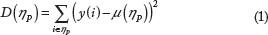
The partition γ^* that maximizes C(γ, η _P ) for all possible partitions is selected for node η _P .

Forest prediction

Using the randomized feature selection process, we fit the tree based on the bootstrap sample {(X₁ Y₁),…, (X _N , Y _N )} generated from the training data. Let Y _i (x) denote the regression tree prediction for input response x corresponding to tree i. The prediction for the RF consisting of T trees denoted by $\widehat{Y}\left(x\right)$ is given by ${\widehat{Y}}_i\left(x\right)=\frac{1}{T}{\sum }_{i=1}^T{\widehat{Y}}_i\left(x\right)$ .

Weighted RF

For comparison purposes, we will also consider the wRF methodology proposed in Ref. 16 that uses empirical values to calculate the weight of the trees. The prediction error of a tree denoted by tPE _j is calculated based on the out-of-bag samples for that tree, and the weight of that tree is estimated as ${\omega }_j=x_j/{\sum }_{j=1}^{ntree}{x}_j$ , where x _j = 1 – tPE _j .

Probabilistic regression trees

Let us consider the generation of regression trees from a probabilistic perspective, which will allow us to utilize well-known concepts of parameter estimations for statistical models. Estimation of regression trees using probability models has been explored in Refs. 5,6. For a regression tree, our goal is to generate the conditional density of the form $P\left(y|x,\phi \right)$ where y and x refers to the output and input responses, respectively, and ϕ denotes the collection of parameters for the tree. The tree splits can be modeled by probabilistic decisions that are conditional on the input x and previous node decisions. As an example, consider the two-level tree shown in Figure 1.

Figure 1

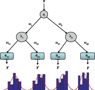
Example of probabilistic decision tree.

The first decision is based on probability P(ω₁|x, η) where ω₁ is the event signifying partition toward the left of the root node and η denotes a parameter vector η = [η₁ T₁].

Note that if we consider

$$P\left(w_1|x,\eta \right)=\frac{e^{{\eta }_1^{T}T1}}{e^{{\eta }_1^{T}X}+e^{{\eta }_1^{T}T1}}+\frac{1}{1+e^{{\eta }_1^T\left(x-T1\right)}}$$

(3)

with large η₁ the split will be close to a sharp linear decision boundary similar to a regression tree. Similarly, we will have

$$P\left({\omega }_2|x,\eta \right)=1-P\left({\omega }_1|x,\eta \right)=\frac{1}{1+e^{{\eta }_1^T\left(T1-x\right)}}$$

(4)

If we consider all the branches of the tree as shown in Figure 1, the corresponding distribution of y conditional on x and tree parameters $\varphi =\left\{\eta ,{\lambda }_1,{\vartheta }_{11},{\vartheta }_{12},{\vartheta }_{21},{\vartheta }_{22}\right\}$ will be given by Eq. 5.

$$\begin{array}{l}P\left(y|x,\varphi \right)\\ =\sum _{i=j}^2\sum _{j=1}^{2}P\left(y|x,{\omega }_{ij},{\lambda }_i,{\omega }_i,\eta \right)P\left({\omega }_{ij}|{\lambda }_i,{\omega }_i,\eta ,x\right)P\left({\omega }_i|\eta ,x\right)\end{array}$$

(5)

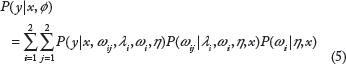
For larger number of branches in the tree, the above technique can be extended to obtain P(y|x, ϕ) for a tree with parameter set ϕ. In this article, we consider that the tree parameters ϕ are generated based on the standard RF node generation criteria given in Eq. 2. The probability distribution at any leaf node is approximated by a Gaussian distribution with mean and variance equal to the mean and variance of the samples at the leaf node. Some examples of empirical distributions fitted to normal approximations are shown in Figure 1.

Consequently, an ensemble of T trees generated by RF regression can be represented by the T tree parameters ϕ₁, ϕ₂,…,ϕ _T with each producing the conditional distribution $P\left(y|x,{\varphi }_i\right)\hspace{0.17em}for\hspace{0.17em}i=1,\mathrm{\dots .}T$ .

Probabilistic Rfs

Mixture distribution

As discussed earlier, we consider the prediction ensemble as a mixture distribution for each sample X _i . Consider an ensemble of T trees where tree j produces the predicted output probability density function P(Y _j |X _i ). The predicted distribution for each tree is based on the estimated probabilistic regression tree model described in the previous section. The probability density function (pdf) P(Y|X _i ) of the forest of T regression trees with weights α₁,…,α _T with α _j ≥ 0 and ${\sum }_{j=1}^T{\alpha }_j=1$ is given by $P\left(Y|X_i\right)={\sum }_{j=1}^T{\alpha }_{j}P\left(Y_j|X_i\right)$ . This approach considers that based on the weights α _j , a tree k will be selected, and the prediction will be decided based on P(Y _k |X _i ).

The mean (μ) of the mixture distribution will be equal to the weighted sum of the distribution means (μ _i ) of the trees as shown in Eq. 6.

$$E\left[Y\right]=\mu =\sum _{i=1}^T{\alpha }_{i,}{\mu }_i$$

(6)

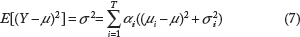
The variance of the mixture distribution (σ ² ) is given by Eq. 7.

$$E\left[{\left(Y-\mu \right)}^2\right]={\sigma }^2=\sum _{i=1}^T{\alpha }_{i,}\left({\left({\mu }_i-\mu \right)}^2+{\sigma }_i^2\right)$$

(7)

Weighted sum of random variables

The mixture distribution approach selects a tree based on the tree weights and then selects a sample output according to the pdf of the tree. Another potential is to consider the weighted sum of realizations from each tree. As discussed earlier, this will be equivalent to considering the output of the forest to be a random variable Z where $Z={\sum }_{j=1}^T{\alpha }_j{Z}_j$ is a weighted sum of T random variables Z₁,…,Z _T where Z _j denotes a random variable with pdf P(Z|X _i based on tree j. The distribution of a sum of random variables can be computed as the convolution of the individual distributions. This scenario is equivalent to analyzing a weighted sum of random variables with different probability density functions, ie, we model the weighted sum of the realizations of the random variables rather than the weighted sum of their distributions as was considered in the first case.

Example for weighted sum of two uncorrelated Gaussian distributions

Consider two independent random variables X₁ and X₂ that are normally distributed with pdfs $N\left(g\mu x_1,{\sigma }_{X_1}^2\right)$ and $N\left(\mu x_2,{\sigma }_{X_2}^2\right)$ , respectively. The distributions of X_1α = α₁X₁ and X_2α = α₂X₂ are given by Eq. 8:

$$\begin{array}{l}f{x}_{1\alpha }\left(x_{1\alpha }\right)=\frac{1}{\sqrt{2\pi {\sigma }_{X1}^2{\alpha }_1^2}}\exp \hspace{0.17em}\frac{\frac{{\left(x_{1\alpha }-{\alpha }_1\mu x_1\right)}^2}{2{\alpha }_1^2{\alpha }_{X_1}^2}}{}\\ f{x}_{2\alpha }\left(x_{2\alpha }\right)=\frac{1}{\sqrt{2\pi {\sigma }_{X2}^2{\alpha }_2^2}}\exp \hspace{0.17em}\frac{\frac{\frac{{\left(x_{2\alpha }-{\alpha }_2\mu x_2\right)}^2}{2{\alpha }_2^2{\alpha }_{X_2}^2}}{}}{}\end{array}$$

(8)

Based on the idea of derived distributions, the pdf of random variable $Z={\alpha }_1{X}_1+{\alpha }_2{X}_2=X_{1\alpha }+X_{2\alpha }$ is given by the convolution of the pdfs of X_1α and X_2α and is given by Eq. 9:

$$fz\left(z\right)={\int }_{-\infty }^{\infty }f{x}_{1\alpha }\left(z-x\right)f{x}_{2\alpha }\left(x\right)dx$$

(9)

Substituting Eq. 8 in Eq. 9, we arrive at:

$$\begin{array}{c}fz\left(z\right)={\int }_{-\infty }^{\infty }\frac{1}{\sqrt{2\pi {\sigma }_{X_1}^2{\alpha }_1^2}}\exp \hspace{0.17em}\frac{\frac{{\left(z-x_{1{\alpha }_1}-{\alpha }_1\mu x_1\right)}^2}{2{\sigma }_{X_1}^2{\alpha }_1^2}}{}\\ \frac{1}{\sqrt{2\pi {\sigma }_{X_2}^2{\alpha }_2^2}}\exp \frac{\frac{{\left(x_{2{\alpha }_2}-{\alpha }_2\mu x_2\right)}^2}{2{\sigma }_{X_2}^2{\alpha }_2^2}}{}\hspace{0.17em}dx\end{array}$$

(10)

$$=\frac{1}{\sqrt{2\pi \left({\sigma }_{X_1}^2{\alpha }_1^2+{\sigma }_{X_2}^2{\alpha }_2^2\right)}}\exp \left[-\frac{{\left(z-\left({\alpha }_1\mu x_1+{\alpha }_2\mu x_2\right)\right)}^2}{2\left({\sigma }_{X_1}^2+{\alpha }_1^2+{\sigma }_{X_2}^2+{\alpha }_2^2\right)}\right]$$

(11)

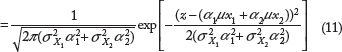
Eq. 11 represents the sum of two independent Gaussian random variables. For T independent Gaussian random variables X₁, X _T with pdfs $N\left({\mu }_1,{\sigma }_1\right),\cdots ,N\left({\mu }_T,{\sigma }_T\right)$ representing the distribution at the T leaf nodes of the forest, the distribution of the random variable Z representing their weighted sum with weights α₁,…, α _T is given by Eq. 12 (derived based on multiple convolutions).

$$f_z\left(z\right)=\frac{1}{\sqrt{2\pi \left({\sum }_{i=1}^T{\sigma }_{X_1}^2{\alpha }_1^2\right)}}\exp \left[-\frac{{\left(z-\left({\sum }_{i=1}^T{\alpha }_1\mu x_1\right)\right)}^2}{2\left({\sum }_{i=1}^T{\sigma }_{X_1}^2+{\alpha }_1^2\right)}\right]$$

(12)

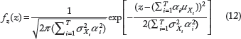
Thus, Z has a normal distribution with $mean={\sum }_{i=1}^T{\alpha }_i,{\mu }_{X_i}$ and $\text{variance}={\sum }_{i=1}^T{\alpha }_i^2{\sigma }_{X_i}^2$ .

However, if the random variables are correlated, ie, the covariance between different tree outputs are nonzero, the mean and variance of Z are given as follows:

$$\text{Mean}\left(\sum _{i=1}^T{\alpha }_1{X}_1\right)=\sum _{i=1}^T{\alpha }_1,{\mu }_1$$

(13)

$$\begin{array}{c}Var\left(\sum _{i=1}^T{\alpha }_i{X}_i\right)=\sum _{i=1}^T\sum _{i=1}^{T}Cov\left({\alpha }_i{X}_i,{\alpha }_j{X}_j\right)\\ =\sum _{i=1}^T{\alpha }_i^{2}Var\left(X_i\right)+2\sum _{1\le i}\sum _{<j\le T}{\alpha }_i{\alpha }_{j}Cov\left(X_i,X_j\right)\end{array}$$

(14)

If the vector C = [α₁,…,α _T ]^′ represent the weight vector and σ represent the T × T covariance matrix, the variance of Z can be represented concisely as

$$Var\left(Z\right)=|C^{\text{'}}\sum C$$

(15)

where C^′ represents the transpose of C.

Note that the mean of Z denotes the weighted sum of the means of individual trees in the forest and the prediction is same as regular RF when the tree weights are equal. The mean of Z remains the same irrespective of whether the trees are correlated or not, whereas the variance of Z is directly related to the covariance of the trees using Eq. 15. In the following sections, we will attempt to estimate the covariance among the trees in a forest and analyze the effect of change in C on the variance of Z.

Empirical measure of correlation between probabilistic trees

The covariance between the trees will be estimated using empirical approaches to arrive at the covariance matrix σ. The i,j position element of σ denotes the covariance between the predictions of ith and jth tree represented by random variables Y _i and Y _j respectively, ie, $\Sigma \left(i,j\right)=E\left[\left(Y_i-E\left(Y_i\right)\right)\left(Y_j-E\left(Y_j\right)\right)\right]$ .

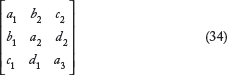
For each input sample X _i , tree j will produce a pdf P(Y _j |X _i ), which will be used to select an output prediction realization y _j . We perform this for all the other trees to arrive at a joint realization of the trees for sample X _i . This is repeated for N input training samples to produce N joint realizations of the random variables Y₁,…,Y _T , which are used to calculate the sample covariance matrix shown in Eq. 34.

$$V=\left[\begin{array}{ccc}\frac{1}{N-1}{\sum }_{i=1}^N{\left(Y_1\left(i\right)-E\left(Y_1\right)\right)}^2& \dots & \frac{1}{N-1}{\sum }_{i=1}^N\left(Y_1\left(i\right)-E\left(Y_1\right)\right)\left(Y_T\left(i\right)-E\left(Y_T\right)\right)\\ ⋮& \ddots & ⋮\\ \frac{1}{N-1}{\sum }_{i=1}^N\left(Y_T\left(i\right)-E\left(Y_T\right)\right)\left(Y_1\left(i\right)-E\left(Y_1\right)\right)& \dots & \frac{1}{N-1}{\sum }_{i=1}^N{\left(Y_T\left(i\right)-E\left(Y_T\right)\right)}^2\end{array}\right]$$

(16)

Effect of tree weight on variance

In this section, we will attempt to generate the lower and upper bounds on CVC where C = [α₁,…,α _T ]^′ represents the tree weight vector. Assuming V is a Hermitian positive definite matrix (note that the covariance matrix V is always positive semidefinite ¹⁷ ), we can generate the Cholesky decomposition ¹⁸ of V = LL ^T , where L is a lower triangular matrix with real and positive diagonal entries. Let the variance of the prediction of a specific forest be given by the function f(C). We have

$$\begin{array}{c}f\left(C\right)=C^{\text{'}}VC\\ =C^{\text{'}}L{L}^{\text{'}}C\\ ={\left(L^{\text{'}}C\right)}^{\text{'}}{L}^{\text{'}}C\\ =A^{\text{'}}A\end{array}$$

(17)

where A = L ^′ C.

Let us analyze the minimum and maximum value of f(C).

$$f\left(C\right)=A^{\text{'}}A{\Vert A\Vert }_2^2={\Vert L^{\text{'}}C\Vert }_2^2\le {\Vert L^{\text{'}}\Vert }_2^2{\Vert C\Vert }_2^2$$

(18)

Since

$${\Vert {\left(L^{\text{'}}\right)}^{-1}{L}^{\text{'}}C\Vert }_2^2\le {\Vert {\left(L^{\text{'}}\right)}^{-1}\Vert }_2^2{\Vert L^{\text{'}}C\Vert }_2^2$$

(19)

and

$${\Vert L^{\text{'}}\Vert }_2^2=\text{maximum}\hspace{0.17em}\text{eigenvalue}\hspace{0.17em}\text{of}\hspace{0.17em}L{L}^{\text{'}}=\max \text{eig}\left(V\right)$$

(20)

$${\Vert {\left(L^{\text{'}}\right)}^{-1}\Vert }_2^2=\frac{1}{\text{maximum}\hspace{0.17em}\text{eigenvalue}\hspace{0.17em}\text{of}\hspace{0.17em}\left(L{L}^{\text{'}}\right)}=\frac{1}{\max \text{eig}\left(V\right)}$$

(21)

We have,

$$\min \text{eig}\left(V\right){\Vert C\Vert }_2^2\le f\left(C\right)\le \max \text{eig}\left(V\right){\Vert C\Vert }_2^2$$

(22)

The minimum for f(C) under the constraint C^′e = 1 where e = [1,1, …, 1]^′ is given by $f\left(C\right)=\frac{1}{e^{\text{'}}{V}^{-1}e}$ . Note that this does not preclude solutions with entries of C being less than zero. The details of the derivation using Lagrange multipliers is included in the Appendix. The weight vector C achieving the minimum is given by $C=\frac{V^{-1}e}{e\text{'}{V}^{-1}e}$ . The computational complexity of estimating the weight vector is $o\left(n^{2.376}\right)$ based on the complexity of matrix inversion using Coppersmith-Winograd algorithm.

Diagonal elements of covariance matrix equal

In the conventional RF model, it is assumed that the trees are uncorrected. Thus, nondiagonal elements of the covariance matrix (which shows the covariance between two different trees) are infinitesimal compared with the diagonal elements (reflecting the variance in the tree). If we ignore the small nondiagonal values and replace them with zeroes, then the covariance matrix (V) is a diagonal matrix. If the variance of the trees are equal $\left(Var\left[X_i\right]=Var\left[X_2\right]=\mathrm{\dots }=Var\left[X_T\right]={\sigma }^2\right)$ , then the covariance matrix (Eq. 34) is a diagonal matrix.

Since the covariance matrix is diagonal with each diagonal entry equal to σ ² , all the T eigenvalues will also be equal to σ ² .

From Eq. 22,

$${\sigma }^2{\Vert C\Vert }_2^2\le f\left(C\right)\le {\sigma }^2{\Vert C\Vert }_2^2$$

(23)

Since |C|₁ = 1 and each entry of C is nonnegative,

$$\min {\Vert C\Vert }_2^2=\frac{T}{T^2}=\frac{1}{T}$$

(24)

Thus from Eq. 23

$$\frac{{\sigma }^2}{T}\le f\left(C\right)$$

(25)

When C^′ = [1/T,1/T,…,1/T] as in a conventional RF scenario, the variance is given by:

$$\left[\frac{1}{T}\hspace{0.17em}\frac{1}{T}\cdots \frac{1}{T}\right]\left[\begin{array}{cccc}{\sigma }^2& 0& \dots & 0\\ 0& {\sigma }^2& \dots & 0\\ ⋮& ⋮& \ddots & ⋮\\ 0& 0& \dots & {\sigma }^2\end{array}\right]\left[\begin{array}{c}\frac{1}{T}\\ ⋮\\ \frac{1}{T}\end{array}\right]=T^{*}\frac{1}{T^2}{\sigma }^2=\frac{{\sigma }^2}{T}$$

(26)

Comparing Eqs. 25 and 26, we observe that C^′ = [1/T, 1/T,…,1/T] achieves the minimum variance for uncorrected trees with equal variance.

Diagonal elements of covariance matrix unequal

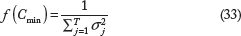
Consider the case where the covariance matrix is a diagonal matrix and the variance of the trees are not equal as shown in Eq. 27.

$$V=\left[\begin{array}{cccc}{\sigma }^2& 0& \dots & 0\\ 0& {\sigma }^2& \dots & 0\\ ⋮& ⋮& \ddots & ⋮\\ 0& 0& \dots & {\sigma }^2\end{array}\right]$$

(27)

where ${\sigma }_i^2$ is the variance of the ith tree. Without loss of generality, assume ${\sigma }_1^2{\Vert C\Vert }_2^2\le f\left(C\right)\le {\sigma }_T^2{\Vert C\Vert }_2^2$ Based on Eq. 22, we have

$${\sigma }_1^2{\Vert C\Vert }_2^2\le f\left(C\right)\le {\sigma }_T^2{\Vert C\Vert }_2^2$$

(28)

Since |C|₁ = 1 and each entry of C ≥ 0,

$$\frac{1}{T}\le {\Vert C\Vert }_2^2\le 1$$

(29)

$$\frac{{\sigma }_1^2}{T}\le f\left(C\right)\le {\sigma }_T^2$$

(30)

When the weights of the trees are equal (ie, C^′ = [1/T, 1/T,…,1/T] we have

$$f\left(C_e\right)=\frac{{\sum }_{i=1}^T{\sigma }_i^2}{T^2}$$

(31)

Thus, there is always a possibility that for some C,

$$f\left(C\right)\le f\left(C_e\right)\frac{{\sigma }_1^2}{T}\le \frac{{\sum }_{i=1}^T{\sigma }_i^2}{T^2}$$

(32)

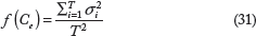
We can show that the minimum f(C_min) in such a scenario is

$$f\left(C_{\min }\right)=\frac{1}{{\sum }_{j=1}^T{\sigma }_j^2}$$

(33)

where $C_{\min }=\left[\frac{1}{{\sum }_{j=1}^T\frac{{\sigma }_1^2}{{\sigma }_j^2}},\dots \frac{1}{{\sum }_{j=1}^T\frac{{\sigma }_T^2}{{\sigma }_j^2}}\right]$ The derivation is included in the Appendix.

Forest with correlated trees

If we consider scenarios where trees are correlated (ie, covariance matrix is not diagonal), placing higher weights on uncorrected trees will result in lower variance. We illustrate this idea intuitively for a forest consisting of three trees.

Consider the covariance matrix for a three-tree forest as

$$\left[\begin{array}{ccc}{a}_1& b_2& c_2\\ b_1& a_2& d_2\\ c_1& d_1& a_3\end{array}\right]$$

(34)

where a₁ ≌ a₂ ≌ a₃ ≌ a, b₁ ≌ b₂ ≌ b, c₁ ≌ c₂ ≌ c, and d₁ ≌ d₂ ≌ d. Consider that the first two trees have high correlation between themselves, while the third tree has little correlation with the other two. Thus, c₁ ≌ c₂ ≌ c ≌ 0 and d₁ ≌ d₂ ≌ d ≌ 0.

The minimum variance will be achieved for $C={\left[\frac{a}{3a+b},\frac{a}{3a+b},\frac{a+b}{3a+b}\right]}^{\text{'}}$ . The details of the derivation are included in the Appendix. Based on numerical weights, we next illustrate the effect of placing higher weight for the third tree on the variance.

Consider $C={\left[\frac{a}{3a+b},\frac{a}{3a+b},\frac{a+b}{3a+b}\right]}^{\text{'}}$ (note that the third tree that is uncorrected to the other trees has higher weight), then the variance of the forest is given by

$$\left[\frac{a}{3a+b},\frac{a}{3a+b},\frac{a+b}{3a+b}\right]\left[\begin{array}{ccc}a& b& 0\\ b& a& 0\\ 0& 0& a\end{array}\right]\left[\begin{array}{c}\frac{a}{3a+b}\\ \frac{a}{3a+b}\\ \frac{a+b}{3a+b}\end{array}\right]=\frac{a\left(a+b\right)}{3a+b}$$

(35)

For a regular RF scenario with equal weights $C=\left[\frac{1}{3}\frac{1}{3}\frac{1}{3}\right]\text{'}$ the variance of the forest is given by

$$\left[\frac{1}{3}\frac{1}{3}\frac{1}{3}\right]\left[\begin{array}{ccc}a& b& 0\\ b& a& 0\\ 0& 0& a\end{array}\right]\left[\begin{array}{c}\frac{1}{3}\\ \frac{1}{3}\\ \frac{1}{3}\end{array}\right]=\frac{\left(3a+2b\right)}{9}$$

(36)

We note that $\frac{\left(3a+2b\right)}{9}-\frac{a\left(a+b\right)}{3a+b}=\frac{2b^2}{9\left(3a+b\right)}>0$ when b > 0. Weights for achieving minimum variance for few more scenarios are derived in the Appendix.

Regression Forest Weight Optimization

In this section, we discuss two approaches to select the weights for the ensemble of trees based on MLE and incorporation of tree correlations.

MLE for mixture model

Consider N independent and identically distributed samples (x _i , y _i ) for i = {1,…,N} used for the generation of the T trees. Let α₁, α _T denote the weights of the trees, then the likelihood (conditional) will be given by:

$$\mathfrak{L}\left(x_1,y_1,\dots x_N,y_N\right)=\prod _{i=1}^N\left(\sum _{j=1}^T{\alpha }_j\left(P(y_1|x_i{\varphi }_j\right)\right)$$

(37)

To ensure that ${\sum }_{j=1}^T{\alpha }_{j}P\left(y_1|x_i{\varphi }_j\right)$ represent a valid probability density function, the weights has to satisfy the following constraints α _i ≥ 0 for i = 1,…,T and ${\sum }_{j=1}^T{\alpha }_j=1$ .

If we denote $P\left(y_i|x_i,{\varphi }_j\right)$ by ${\xi }_{i,j}$ for i = 1,2,…,N samples and j = 1,…,T trees, a compact form of representation of the likelihood of the samples as an N length vector $f={\left[f_1,\cdots ,f_N\right]}^T$ is $f=\xi \alpha$ :

$$\left[\begin{array}{c}{f}_1\\ \cdot \\ \cdot \\ f_N\end{array}\right]=\left|\begin{array}{ccc}{\xi }_{1,1}& \dots & {\xi }_{1,K}\\ & \dots & \\ & \dots & \\ {\xi }_{N,1}& \dots & {\xi }_{N,K}\end{array}\right|\left[\begin{array}{c}{\alpha }_1\\ \cdot \\ \cdot \\ {\alpha }_K\end{array}\right]$$

The goal is to maximize the product ${\prod }_{i=1}^N{f}_i$ with constraints α ≥ 0 and ${\sum }_{j=1}^K{\alpha }_j-1=0$ .

We solve this optimization problem using Matlab fmincon function that utilizes an interior point approach to find the minimum of a constrained nonlinear function.

Weight distribution based on correlation of trees for weighted sum of random variables model

Among T trees in the forest, consider that some of the trees can have higher correlation between themselves which can be clustered as groups with high correlations among the trees in a group but have limited correlation between trees in different groups. The purpose is to provide higher weight to the uncorrelated trees as compared with the correlated trees. The algorithmic pseudo code is shown as Algorithm 1.

Algorithm 1.

Algorithmic representation of weight selection

STEP 1: Cluster Trees Based on Correlations

STEP 2: Let the k clusters be $\left[{\alpha }_1,\dots ,{\alpha }_{{\rho }_1}\right],.,\left[{\alpha }_{T-{\rho }_k}\dots ,{\alpha }_T\right]$

STEP 3: Assign equal weight $\frac{1}{k}$ to each cluster ie, assign weight $\frac{1}{{\rho }_r^k}$ to each tree in cluster r

To achieve the clustering of the trees, we have applied hierarchical clustering with inverse of the covariance between trees as the distance criteria and linkages between clusters decided based on the minimum distance among pairs belonging to the two clusters (single-linkage clustering). The pair of trees that have the smallest distance among all pairs is linked first followed by the next pair and so on. An example of hierarchical ordering with six trees is shown in Figure 2. To generate the final clusters, we have applied a threshold for the inverse covariance and all links below the threshold are considered as separate clusters. The threshold has been taken to be 60% of the average variance of the trees or in other words $\text{threshold}=\frac{0.6}{T}tr(\sum )$ where tr(σ) denotes the trace of the covariance matrix. As an example, consider the hierarchical ordering in Figure 2 with a threshold of 3.8, which will result in four separate cluster of trees [2,3], [4,5], [1], and [6].

Figure 2

Example of hierarchical clustering.

Results

Synthetic dataset

ML estimate for mixture model

To evaluate the performance of our algorithm as compared with competing methodologies, we created a synthetic dataset consisting of 100 × 10 size predictor matrix X and 100 × 1 size response vector Y. The predictor variables are randomly generated based on a [0 1] uniform distribution. The response variable is generated based on the predictor variables using Eq. 38 where N₁ denotes a random noise with pdf ℕ(0,1).

$$\begin{array}{c}{Y}_1=5x_3+5x_9-1.5x_1^3+x_2\\ *x_4+2x_5+10x_6-1.5x_7^2+x_6*x_8+2N_1\end{array}$$

(38)

One of our objectives is to check if we are able to reduce the mean square error (MSE) in prediction along with lowering the width of the CI by using MLE of the tree weights. From henceforth, the probabilistic RF with tree weights generated by MLE will be termed as PRF and the probabilistic RF with equal tree weights will be denoted as RF. The weighted random forest approach ¹⁶ will be denoted by wRF.

To report our results, we have used 75 samples (75%) for training and the remaining 25 samples (25%) for testing (holdout validation) and compared Pearson correlation coefficients, mean absolute error (MAE), MSE, normalized root mean square error (NRMSE), and width of the CI between predicted and experimental responses for RF, wRF, and PRF models. NRMSE of output response can be calculated as:

$$\text{NRMSE}=\sqrt{\frac{{\left(y-\widehat{y}\right)}^T\left(y-\widehat{y}\right)}{\left(y-1\cdot E{\left(y\right)}^T\left(y-1\cdot E\left(y\right)\right)\right)}}$$

(39)

where y and ŷ denote the vector of actual and predicted drug sensitivities, respectively, and $\mathbb{E}(y)$ denote the expectation of vector y. We have considered different number of trees to build the models (RF, wRF, and PRF) and the change in MAE, NRMSE, and correlation coefficients between actual and predicted values for these models are shown in Table 1. Table 1 shows that the prediction errors measured in terms of MAE and NRMSE are smaller with PRF as compared with wRF and RF for different number of trees in the forest. We observe analogous behavior based on a similarity measure with PRF correlation coefficient between predicted and experimental values to be higher than wRF and RF.

Table 1

MAE, NRMSE, and correlation between actual and predicted responses for 100 samples for different number of trees in the forest.

TREE	MAE			NRMSE			CORRELATION
	RF	wRF	PRF	RF	wRF	PRF	RF	wRF	PRF
5	0.1437	0.1431	0.1357	0.7785	0.7759	0.7565	0.6560	0.6600	0.6681
10	0.1126	0.1129	0.1044	0.7623	0.7645	0.7326	0.6535	0.6507	0.6848
20	0.0937	0.0943	0.0876	0.7103	0.7127	0.6747	0.7435	0.7402	0.7627
30	0.1319	0.1318	0.1195	0.6383	0.6371	0.6051	0.8169	0.8188	0.8217
50	0.1240	0.1239	0.1109	0.6737	0.6738	0.6394	0.8151	0.8169	0.8499

Note: Minimum leaf size is 3 and 5 features considered for each split.

The previous measures are based on the mean of the predicted pdf and actual observation. We also consider a probabilistic measure to capture where an actual observation lies in comparison with the predicted pdf. Similar to P-value for doubled tailed event, we considered the probability η(y _i ) of observing results more extreme than y _i when our prediction probability density function is given by the pdf of Ŷ.

$$\eta \left(y_i\right)=2\times \min \left\{\mathrm{Pr}\left(\widehat{Y}\le y_i\right),\mathrm{Pr}\left(\widehat{Y}\ge y_i\right)\right\}$$

(40)

A higher value of η(y _i ) will denote that we cannot reject the hypothesis that the observed responses are from the predicted distributions. A higher value of $\mathbb{E}(\eta (y_i))$ , where the expectation is over the testing samples, will be preferable for model comparisons. Table 2 shows $\mathbb{E}(\eta (y_i))$ for different number of trees for RF, wRF, and PRF. Based on Table 2, we observe that $\mathbb{E}(\eta (y_i))$ for PRF is higher than both wRF and RF.

Table 2

$\mathbb{E}(\eta (y_i))$ for different number of trees in the forest.

TREE	E(η(y i ))
	RF	wRF	PRF
5	0.5596	0.5586	0.5617
10	0.6467	0.6467	0.6655
20	0.7049	0.7034	0.7226
30	0.6328	0.6335	0.6281
50	0.6043	0.6042	0.6303

Note: Minimum leaf size is 3 and 5 features considered for each split.

We report the percentage difference in the width of the CI at different confidence levels (CLs) for PRF as compared with RF and wRF in Table 3. An M% change in the width of the CI denotes that on an average, PRF generated CI is M% lower than the RF generated CI. We observe that the average width of the CI for PRF is lower than RF and wRF for all CLs and different number of trees.

Table 3

Change in CI width for different CLs between RF and PRF and wRF and PRF model for 100 samples for different number of trees in the forest.

TREE	% DECREASE IN MEAN CI COMPARED TO RF					% DECREASE IN MEAN CI COMPARED TO wRF
	50%	70%	80%	95%	99%	50%	70%	80%	95%	99%
	CL	CL	CL	CL	CL	CL	CL	CL	CL	CL
5	7.52	9.29	10.13	8.99	6.31	6.49	8.06	8.57	8.20	5.79
10	0.14	0.63	0.78	1.55	1.98	0.72	0.81	1.00	1.55	1.92
20	3.16	2.43	1.93	0.73	0.50	3.16	2.34	1.78	0.64	0.34
30	12.78	13.45	12.53	9.65	7.54	12.92	13.36	13.01	9.65	7.56
50	3.94	2.61	2.55	1.41	1.65	3.79	2.43	2.48	1.32	1.74

Note: Minimum leaf size is 3 and 5 features considered for each split.

Table 4 shows the NRMSE and correlation coefficient between actual and predicted responses for RF, wRF, and PRF and percentage change in the width of CI with PRF as compared with RF for a simulation with 250 samples. Similar to the previous results with 100 samples, we observe improvement with PRF as compared with both RF and wRF with respect to NRMSE and correlation coefficient between actual and predicted responses. The results also show that the NRMSE has decreased for all the approaches when the sample size has been increased to 250 samples as compared to 100 samples. The absolute difference in performance for PRF as compared with RF and wRF is better for 100 samples, but the percentage improvement in performance is similar for both the sample scenarios.

Table 4

NRMSE, correlation between actual and predicted output, and change in CI width for different CLs for 250 samples for different number of trees in the forest.

TREE							% DECREASE IN MEAN CI WITH PRF COMPARED TO RF
	NRMSE			CORRELATION			DIFFERENT CONFIDENCE LEVEL
	RF	wRF	PRF	RF	wRF	PRF	50%	70%	80%	95%	99%
5	0.5880	0.5871	0.5710	0.8177	0.8182	0.8240	4.66	4.36	4.63	4.61	4.02
10	0.5503	0.5498	0.5299	0.8396	0.8400	0.8529	4.19	4.45	3.92	3.26	2.87
20	0.5746	0.5750	0.5681	0.8243	0.8241	0.8302	3.86	3.07	2.77	2.60	2.79
30	0.5830	0.5832	0.5809	0.8180	0.8178	0.8185	1.36	1.34	1.51	1.35	1.26
50	0.5821	0.5826	0.5626	0.8259	0.8258	0.8380	4.19	3.15	2.90	2.73	2.89

Note: Minimum leaf size is 3 and 5 features considered for each split.

Weighted sum of random variables

In this section, we consider the effect of tree weights on the MSE and prediction variance for the weighted sum of random variables scenario. We generated a synthetic feature matrix of 500 samples and 1000 features based on a uniform probability distribution [0 1]. The output response has been generated based on Eq. 38 where the output response is dependent on nine of the input features. A random set of 300 of these 500 samples have been used for training, while the remaining 200 samples have been used for testing. We have used the filter feature selection approach RRelieff ¹⁹ to reduce the initial set of 1000 features to 100 (10 among these 100 are randomly considered for each node splitting) for training the regression trees.

We have considered five trees for the generation of the RF model, and the covariance matrix for the five trees based on the training samples is given by Eq. 41. We have used smaller number of trees for easy visualization of the covariance matrix along with concise analysis of the inferred weights.

$$V=\left[\begin{array}{ccccc}0.0322& \text{0}.\text{0146}& 0.0137& 0.0126& 0.0166\\ 0.0151& 0.0396& \text{0}.\text{0202}& \text{0}.\text{0178}& 0.0231\\ 0.0135& 0.0202& \text{0}.\text{0357}& \text{0}.\text{0133}& 0.0174\\ 0.0126& 0.0178& \text{0}.\text{0133}& \text{0}.\text{0336}& 0.0183\\ 0.0170& 0.0238& 0.0177& \text{0}.\text{0178}& 0.0390\end{array}\right]$$

(41)

In Eq. 41, the diagonal elements are the variance of each tree with itself, while the nondiagonal elements are covariance between different trees. We note that the covariance between trees 2 and 5 is high compared with the other covariances. By applying hierarchical clustering with inverse covariance as the distance measure and 60% of average variance as threshold, we arrive at four clusters: [2, 5], [1], [3], [4]. We assign equal weights to each cluster (0.25), and where there is more than one tree in a cluster, the weight is equally divided among the trees in the cluster. Thus, we arrive at the following weight vector for PRF model C = [0.25 0.125 0.25 0.25 0.125].

Since we considered holdout validation for variance comparison, we generated the covariance among the trees for the testing samples (denoted by σ) which is shown in Eq. 42.

$$\sum =\left[\begin{array}{ccccc}0.0363& \text{0}.\text{0033}& -0.0025& 0.0029& 0.0045\\ 0.0036& 0.0366& \text{0}.\text{0008}& \text{0}.\text{0030}& 0.0132\\ -0.0033& 0.0006& \text{0}.\text{0348}& \text{0}.\text{0008}& -0.0008\\ 0.0030& 0.0032& \text{0}.\text{0018}& \text{0}.\text{0330}& 0.0001\\ 0.0043& 0.0120& -0.0010& \text{0}.\text{0002}& 0.0379\end{array}\right]$$

(42)

Consequently, the variance of the forest with equal tree weights is given by

$$\begin{array}{l}\left[1/5\hspace{0.17em}1/5\text{}\hspace{0.17em}1/5\hspace{0.17em}1/5\hspace{0.17em}1/5\right]*\sum \\ \hspace{0.17em}*{\left[1/5\hspace{0.17em}1/5\hspace{0.17em}1/5\hspace{0.17em}1/5\hspace{0.17em}1/5\hspace{0.17em}\right]}^{\text{'}}=0.092\end{array}$$

(43)

whereas the variance of the forest based on our weight selection is given by

$$C*\sum *C^{\text{'}}=0.089$$

(44)

The above results illustrate that for the weighted sum of random variables scenario, the variance of the forest prediction can be reduced by generating the weight of the trees based on tree clusters as compared with using equal weights for all trees.

ML estimate of mixture model applied to CCLE dataset

CCLE dataset has been downloaded from http://www.broadinstitute.org/ccle/home. CCLE dataset has two types of genetic characterization information: (i) gene expression and (ii) single-nucleotide polymorphism (SNP6). Gene expression has been downloaded from CCLE_Expression_Entrez_2012-09-29.gct. In this dataset, there are 18,988 gene features with no missing values for 1037 cell lines. The SNP6 dataset has been extracted from CCLE_copynumber_ayGene_2013-12-03.txt. For 1043 cell lines, there are 23,316 features. For our experiments, we have selected 1012 cell lines that are common to both gene expression and SNP6 dataset.

The drug sensitivity data has been downloaded from the addendum published by Barretina et al. ²⁰ The data provide 24 drug responses for 504 cell lines. Drug sensitivity data of the area under the curve have been collected from Act Area and normalized to [0 1]. The SNP6 and gene expression data integrated model was constructed based on individual RF models combined with a linear regression stacking approach. ³

CI and variance

For the calculation of the CI, we have considered 15 drugs in the CCLE database and considered samples with drug sensitivity higher than 0.1 so as to have noticeable variance among the output responses. The number of samples used for the experiments for the 15 drugs varies from 70 to 395. We have used fivefold cross-validation for all our computations, where the data samples are randomly partitioned into five equal parts and four parts are used for training and the remaining part used for testing and the process repeated five times corresponding to the five different testing partitions.

Based on the model inferred from the training samples, the mean and variance of the output of the leaf node for the testing set has been calculated. Thus, for a testing set of 20 samples and 10 trees, we have a matrix of mean and variance of size 20 × 10. Based on the calculated means and variances, a Gaussian mixture distribution has been derived. Cumulative distribution function has been eventually derived from this distribution to calculate the CIs for different CLs.

To analyze the estimated CIs, we have considered the ratio of the number of experimental testing responses contained in the predicted CI to the total number of testing samples. We will term the ratio as the coverage probability of the CI. Note that we are calculating the coverage probability from cross-validation data as compared with resubstitution data, and thus, there can be significant differences from the CI level for limited samples.

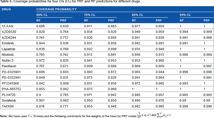
The coverage probability for different CLs for all the 15 drugs is shown in Table 5. We observe that the RF and PRF coverage probabilities are quite similar and PRF coverage probability is closer to the actual CL than the RF coverage probability. As expected, the coverage probability is increasing with the increase in CL for both RF and PRF model.

Table 5

Coverage probabilities for four CIs (CL) for PRF and RF predictions for different drugs.

DRUG	COVERAGE PROBABILITY
	50% CL		70% CL		80% CL		95% CL
	RF	PRF	RF	PRF	RF	PRF	RF	PRF
	17-AAG	0.686	0.650	0.911	0.883	0.977	0.959	1	1
	AZD0530	0.829	0.764	0.934	0.929	0.949	0.959	0.994	0.989
AZD6244	0.743	0.712	0.920	0.893	0.951	0.938	0.991	0.986
Erlotinib	0.844	0.836	0.931	0.939	0.982	0.991	0.991	1
Lapatinib	0.838	0.788	0.932	0.898	0.974	0.949	1	1
Nilotinib	0.795	0.742	0.913	0.881	0.956	0.913	0.986	0.989
Nutlin-3	0.872	0.825	0.941	0.953	0.953	0.965	1	1
Paclitaxel	0.707	0.671	0.909	0.886	0.969	0.959	1	0.997
PD-0325901	0.686	0.665	0.893	0.872	0.965	0.944	0.996	0.996
PD-0332991	0.849	0.831	0.973	0.929	0.991	0.964	1	0.991
PF2341066	0.842	0.808	0.931	0.938	0.972	0.965	0.993	1
PHA-665752	0.855	0.842	0.973	0.960	1	1	1	1
PLX4720	0.9	0.785	0.971	0.942	0.985	0.957	0.985	0.985
Sorafenib	0.901	0.862	0.950	0.950	0.980	0.970	0.99	0.99
TAE684	0.816	0.771	0.955	0.948	0.982	0.965	0.996	0.996

Note: We have used T = 10 trees and the following constraints for the weights of the trees for PRF model $\frac{1}{3T}\le {\alpha }_i\le 1$ and ${\sum }_{j=1}^T{\alpha }_j=1$ .

For the results shown in Table 5, we also calculated the P-values of paired t-test between PRF and RF predictions and actual responses. The P-values of paired t-test between (a) PRF prediction and actual responses turned out to be 0.6172 and between (b) RF prediction and actual responses turned out to be 0.6052. A higher value for the PRF scenario represents that the PRF predictions are closer to the actual responses as compared with the RF predictions.

The change in coverage probability with the number of trees (T) for drug 17-AAG is shown in Table 6. We observe that the coverage probabilities are closer to the actual CLs with lower number of trees. However, the increase in the number of trees in the forest produces lower variance and higher prediction accuracy.

Table 6

Coverage probabilities for four CIs for different number of trees (from 2 to 100) for drug 17-AAG with 395 samples.

NO. OF TREES	COVERAGE PROBABILITY
	50% CL		70% CL		80% CL		95% CL
	RF	PRF	RF	PRF	RF	PRF	RF	PRF
T = 2	0.6532	0.6228	0.8228	0.8101	0.8911	0.8886	0.9848	0.9873
T = 5	0.6937	0.6658	0.9038	0.8861	0.9570	0.9418	0.9975	0.9949
T = 10	0.686	0.650	0.911	0.883	0.977	0.959	1	1
T = 20	0.7089	0.6886	0.9139	0.9089	0.9747	0.9722	1	1
T = 100	0.7291	0.7241	0.9342	0.9266	0.9823	0.9772	1	1

Note: Results for both RF and PRF models show similar type of behavior.

From Tables 5 and 6, we observe that both RF and PRF provide similar coverage probabilities for the generated CIs.

We next analyzed the error in prediction using different error metrics (MSE, MAE, and NRMSE) and the length of the CIs for PRF in comparison with RF and wRF ¹⁶ .

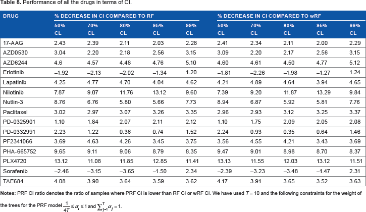
We first explored whether PRF in comparison with RF and wRF can reduce prediction error (as measured by different metrics) while decreasing the CI in majority of the cases. The ratio of the number of testing samples, where the PRF model-generated CI is lower than the RF model-generated CI, to all samples is defined as PRF CI ratio. For example, a PRF CI ratio of 0.60 will denote that for 60% of the testing samples, PRF model-generated CI is lower than RF model-generated CI.

The MSE, MAE, and NRMSE for different drugs are shown in Table 7, while Table 8 shows the PRF CI ratio in comparison with RF and wRF for different CLs. Tables 7 and 8 show that the average errors for PRF in comparison with RF and wRF is similar based on multiple error metrics, whereas the PRF CI ratio is >0.5 (between 0.54 and 0.6) for all CLs. Thus, the results support the idea that as compared with using equal weights for all trees, weight optimization using MLE can potentially predict drug sensitivity with higher confidence while maintaining similar error. Figure 3 represents two example pdfs generated by PRF and RF, which shows that the PRF predicted distribution has lower variance as compared with RF, while maintaining similar mean.

Figure 3

RF generated PDF is more spread out than PRF generated pdf, which implies that the CI of RF generated pdf is higher than PRF generated pdf.

Table 7

Performance of all the drugs in terms of MSE, MAE, and NRMSE.

DRUG	MSE			MAE			NRMSE
	RF	wRF	PRF	RF	wRF	PRF	RF	wRF	PRF
17-AAG	0.0175	0.0167	0.0185	0.1075	0.1051	0.1108	1.0055	0.9828	1.0363
AZD0530	0.0071	0.0066	0.0078	0.0628	0.0605	0.0650	1.0023	0.9637	1.0502
AZD6244	0.0157	0.0160	0.0169	0.0983	0.1018	0.1011	0.9567	0.9642	0.9946
Erlotinib	0.0047	0.0049	0.0057	0.0513	0.0528	0.0573	0.9956	1.0021	1.0894
Lapatinib	0.0070	0.0073	0.0079	0.0629	0.0616	0.0649	0.9799	0.9992	1.0418
Nilotinib	0.0241	0.0226	0.0230	0.1015	0.0931	0.0974	1.0326	1.0021	1.0116
Nutlin-3	0.0034	0.0038	0.0037	0.0435	0.0449	0.0438	0.9762	1.0415	1.0296
Paclitaxel	0.0237	0.0236	0.0243	0.1226	0.1240	0.1257	0.9229	0.9205	0.9354
PD-0325901	0.0259	0.0254	0.0279	0.1312	0.1306	0.1364	0.9534	0.9446	0.9873
PD-0332991	0.0053	0.0045	0.0058	0.0573	0.0524	0.0609	0.9825	0.9139	1.0379
PF2341066	0.0075	0.0074	0.0060	0.0646	0.0603	0.0564	1.0578	1.0458	0.9519
PHA-665752	0.0039	0.0039	0.0039	0.0509	0.0497	0.0488	1.0667	1.0700	1.0616
PLX4720	0.0100	0.0107	0.0106	0.0730	0.0775	0.0720	1.0011	1.0270	1.0283
Sorafenib	0.0072	0.0069	0.0063	0.0568	0.0533	0.0505	1.0471	1.0309	0.9923
TAE684	0.0087	0.0075	0.0089	0.0696	0.0644	0.0707	0.9682	0.8957	0.9759
Average	0.0114	0.0112	0.0118	0.0769	0.0755	0.0774	0.9966	0.9869	1.0149

Note: We have used T = 10 and the following constraints for the weight of the trees for the PRF model $\frac{1}{4T}\le {\alpha }_i\le 1$ and ${\sum }_{j=1}^T{\alpha }_j=1$ .

Table 8

Performance of all the drugs in terms of CI.

DRUG	% DECREASE IN CI COMPARED TO RF					% DECREASE IN CI COMPARED TO wRF
	50% CL	70% CL	80% CL	95% CL	99% CL	50% CL	70% CL	80% CL	95% CL	99% CL
	17-AAG	2.43	2.39	2.11	2.03	2.28	2.41	2.34	2.11	2.00	2.29
AZD0530	3.04	2.20	2.18	2.56	3.15	3.09	2.20	2.17	2.56	3.15
AZD6244	4.6	4.57	4.48	4.76	5.10	4.60	4.61	4.50	4.77	5.12
Erlotinib	–1.92	–2.13	–2.02	–1.34	1.20	–1.81	–2.26	–1.98	–1.27	1.24
Lapatinib	4.25	4.77	4.70	4.04	4.62	4.21	4.89	4.64	3.94	4.65
Nilotinib	7.87	9.07	11.76	13.12	9.60	7.39	9.20	11.87	13.29	9.84
Nutlin-3	8.76	6.76	5.80	5.66	7.73	8.94	6.87	5.92	5.81	7.76
Paclitaxel	3.02	2.97	3.07	3.26	3.35	2.96	2.93	3.12	3.25	3.37
PD-0325901	1.10	1.84	2.07	2.11	2.12	1.10	1.75	2.09	2.05	2.08
PD-0332991	2.23	1.22	0.36	0.74	1.52	2.24	0.93	0.35	0.64	1.46
PF2341066	3.69	4.63	4.26	3.45	3.75	3.56	4.55	4.21	3.43	3.69
PHA-665752	9.65	9.11	9.06	8.79	8.35	9.47	9.01	8.98	8.70	8.37
PLX4720	13.12	11.08	11.85	12.85	11.41	13.13	11.55	12.03	13.12	11.51
Sorafenib	–2.46	–3.15	–3.65	–1.50	2.34	–2.39	–3.23	–3.48	–1.47	2.31
TAE684	4.08	3.90	3.64	3.59	3.62	4.17	3.91	3.65	3.52	3.63

Notes: PRF CI ratio denotes the ratio of samples where PRF CI is lower than RF CI or wRF CI. We have used T = 10 and the following constraints for the weight of the trees for the PRF model $\frac{1}{4T}\le {\alpha }_i\le 1$ and ${\sum }_{j=1}^T{\alpha }_j=1$ .

The percentage decreases in mean CI with PRF as compared with RF and wRF are shown in Table 9. We note that the average CI for PRF is lower than RF and wRF in an overwhelming majority of cases.

Table 9

Percentage decrease in mean CI with PRF as compared with RF and wRF for 15 drugs of CCLE dataset.

DRUG	% DECREASE IN CI COMPARED TO RF					% DECREASE IN CI COMPARED TO wRF
	50% CL	70% CL	80% CL	95% CL	99% CL	50% CL	70% CL	80% CL	95% CL	99% CL
	17-AAG	2.43	2.39	2.11	2.03	2.28	2.41	2.34	2.11	2.00	2.29
AZD0530	3.04	2.20	2.18	2.56	3.15	3.09	2.20	2.17	2.56	3.15
AZD6244	4.6	4.57	4.48	4.76	5.10	4.60	4.61	4.50	4.77	5.12
Erlotinib	–1.92	–2.13	–2.20	–1.34	1.20	–1.84	–2.26	–1.98	–1.27	1.24
Lapatinib	4.25	4.77	4.70	4.04	4.62	4.21	4.89	4.64	3.94	4.65
Nilotinib	7.87	9.07	11.76	13.12	9.60	7.39	9.20	11.87	13.29	9.84
Nutlin-3	8.76	6.76	5.80	5.66	7.73	8.94	6.87	5.92	5.81	7.76
Paclitaxel	3.02	2.97	3.07	3.26	3.35	2.96	2.93	3.12	3.25	3.37
PD-0325901	1.10	1.84	2.07	2.11	2.12	1.10	1.75	2.09	2.05	2.08
PD-0332991	2.23	1.22	0.36	0.74	1.52	2.24	0.93	0.35	0.64	1.46
PF2341066	3.69	4.63	4.26	3.45	3.75	3.56	4.55	4.21	3.43	3.69
PHA-665752	9.65	9.11	9.06	8.79	8.35	9.47	9.01	8.98	8.70	8.37
PLX4720	13.12	11.08	11.85	12.85	11.41	13.13	11.55	12.03	13.12	11.51
Sorafenib	–2.46	–3.15	–3.65	–1.50	2.34	–2.39	–3.23	–3.48	–1.47	2.31
TAE684	4.08	3.90	3.64	3.59	3.62	4.17	3.91	3.65	3.52	3.63

Notes: Number of features used for each split is 10, minimum number of samples in a leaf node = 5, T = 10 and PRF constraints $\frac{1}{4T}\le {\alpha }_i\le 1$ and ${\sum }_{j=1}^T{\alpha }_j=1$ .

We also compared our approach with quantile regression forests (QRFs) ²¹ that uses nonparametric empirical distributions to model the distributions at the leaf nodes. We observed (results not included) that QRFs can produce smaller CIs than RF and PRF but the coverage probability of PRF is significantly lower. It appears that the empirical distributions based on a few samples can provide smaller variance but has limited coverage that defeats the purpose of designing the CIs.

Prior feature selection

In this experiment, we have used filter feature selection algorithm RRelieff ¹⁹ to reduce the initial set of features used for training the RF, PRF, and wRF models. We have considered the CCLE cell lines that are common to all 15 drugs resulting in 396 samples. Features election has been used to reduce the number of features to 50 for each dataset.

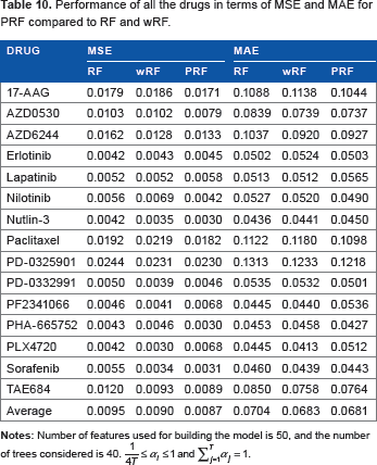
Table 10 shows the average errors in terms of MSE and MAE for the 15 drugs with 50 selected features for RF, wRF, and PRF. We observe that PRF performs better in comparison with RF and wRF in terms of both average MSE and MAE.

Table 10

Performance of all the drugs in terms of MSE and MAE for PRF compared to RF and wRF.

DRUG	MSE			MAE
	RF	wRF	PRF	RF	wRF	PRF
17-AAG	0.0179	0.0186	0.0171	0.1088	0.1138	0.1044
AZD0530	0.0103	0.0102	0.0079	0.0839	0.0739	0.0737
AZD6244	0.0162	0.0128	0.0133	0.1037	0.0920	0.0927
Erlotinib	0.0042	0.0043	0.0045	0.0502	0.0524	0.0503
Lapatinib	0.0052	0.0052	0.0058	0.0513	0.0512	0.0565
Nilotinib	0.0056	0.0069	0.0042	0.0527	0.0520	0.0490
Nutlin-3	0.0042	0.0035	0.0030	0.0436	0.0441	0.0450
Paclitaxel	0.0192	0.0219	0.0182	0.1122	0.1180	0.1098
PD-0325901	0.0244	0.0231	0.0230	0.1313	0.1233	0.1218
PD-0332991	0.0050	0.0039	0.0046	0.0535	0.0532	0.0501
PF2341066	0.0046	0.0041	0.0068	0.0445	0.0440	0.0536
PHA-665752	0.0043	0.0046	0.0030	0.0453	0.0458	0.0427
PLX4720	0.0042	0.0030	0.0068	0.0445	0.0413	0.0512
Sorafenib	0.0055	0.0034	0.0031	0.0460	0.0439	0.0443
TAE684	0.0120	0.0093	0.0089	0.0850	0.0758	0.0764
Average	0.0095	0.0090	0.0087	0.0704	0.0683	0.0681

Notes: Number of features used for building the model is 50, and the number of trees considered is 40. $\frac{1}{4T}\le {\alpha }_i\le 1$ and ${\sum }_{j=1}^T{\alpha }_j=1$ .

The prediction performance can also be measured in terms of the bias and variance of the error distributions produced by different predictive models. The bias will be an inverse measure of accuracy, and variance will be an inverse measure of precision. Table 11 shows the bias and variance for RF, wRF, and PRF for different drugs. We note that the average absolute bias (measure of inaccuracy) is lower for PRF (0.0014) as compared with RF (0.0020) and wRF (0.0025). Similarly, the variance (measure of imprecision) for PRF (0.0087) is smaller than variances for RF (0.0096) and wRF (0.0090).

Table 11

Performance of all the drugs in terms of bias and variance for PRF compared with RF and wRF.

DRUG	BIAS			VARIANCE
	RF	wRF	PRF	RF	wRF	PRF
17-AAG	0.0023	0.0087	0.0020	0.0182	0.0187	0.0173
AZD0530	–0.0055	–0.0150	–0.0005	0.0104	0.0101	0.0080
AZD6244	–0.0133	0.0190	0.0037	0.0162	0.0126	0.0135
Erlotinib	0.0054	0.0110	–0.0054	0.0042	0.0042	0.0045
Lapatinib	–0.0116	–0.0080	–0.0142	0.0052	0.0052	0.0057
Nilotinib	–0.0062	0.0002	0.0012	0.0057	0.0070	0.0043
Nutlin-3	–0.0102	0.0020	–0.0057	0.0042	0.0036	0.0031
Paclitaxel	0.0040	0.0192	0.0351	0.0194	0.0217	0.0171
PD-0325901	0.0086	0.0025	–0.0048	0.0246	0.0234	0.0232
PD-0332991	0.0118	0.0064	0.0083	0.0050	0.0039	0.0047
PF2341066	0.0012	–0.0053	–0.0003	0.0047	0.0041	0.0069
PHA-665752	–0.0045	–0.0108	0.0058	0.0044	0.0046	0.0030
PLX4720	–0.0027	0.0030	–0.0038	0.0042	0.0030	0.0069
Sorafenib	–0.0081	0.0005	–0.0028	0.0055	0.0034	0.0032
TAE684	–0.0009	0.0048	0.0030	0.0122	0.0094	0.0090
Average	–0.0020	0.0025	0.0014	0.0096	0.0090	0.0087

Notes: Number of features used for building the model is 50, and the number of trees considered is 40. $\frac{1}{4T}\le {\alpha }_i\le 1$ and ${\sum }_{j=1}^T{\alpha }_j=1$ .

The results given in Tables 10 and 11 show that the PRF provides improvement in terms of average error, accuracy, and precision. We next consider the length of the CI with PRF as compared with RF and wRF Table 12 shows that the percentage decrease in average CI for PRF when compared with RF and wRF is positive for majority of the drugs.

Table 12

Performance of all the drugs in terms of % decrease in mean CI with PRF as compared with RF and wRF.

DRUG	% DECREASE IN CI COMPARED TO RF					% DECREASE IN CI COMPARED TO wRF
	50% CL	70% CL	80% CL	95% CL	99% CL	50% CL	70% CL	80% CL	95% CL	99% CL
17-AAG	2.79	2.37	2.48	2.59	2.54	2.87	2.38	2.52	2.61	2.54
AZD0530	3.10	2.47	2.86	2.52	3.40	3.11	2.35	2.98	2.58	3.37
AZD6244	1.52	1.68	1.88	0.87	0.70	1.53	1.83	1.79	0.93	0.79
Erlotinib	3.02	2.13	1.75	1.37	1.63	3.03	2.17	1.76	1.39	1.64
Lapatinib	1.49	1.34	1.29	1.02	1.97	1.37	1.31	1.29	0.96	1.95
Nilotinib	1.62	0.64	0.49	2.12	4.50	1.44	0.57	0.44	2.13	4.49
Nutlin-3	0.01	–0.61	–1.01	–1.18	0.06	0.07	–0.65	–1.01	–1.14	0.08
Paclitaxel	3.92	2.91	2.38	1.92	2.03	3.90	2.79	2.48	1.91	2.01
PD-0325901	–0.09	–0.07	–0.03	–0.49	–0.40	0.00	–0.01	–0.06	–0.43	–0.41
PD-0332991	3.38	3.13	2.58	1.65	2.35	3.39	3.13	2.55	1.57	2.29
PF2341066	5.76	6.09	5.08	5.06	5.88	5.82	6.02	5.15	5.05	5.80
PHA-665752	1.83	0.97	0.37	–0.59	–0.23	1.76	0.93	0.37	–0.66	–0.23
PLX4720	0.80	0.59	0.97	–0.23	0.04	0.80	0.64	0.94	–0.20	0.01
Sorafenib	3.95	4.16	3.57	2.81	4.33	3.95	4.29	3.55	2.87	4.32
TAE684	0.61	0.40	0.02	–0.68	–0.33	0.70	0.44	0.02	–0.62	–0.33

Notes: Number of features used for building the model is 50, and the number of trees considered is 40. $\frac{1}{4T}\le {\alpha }_i\le 1$ and ${\sum }_{j=1}^T{\alpha }_j=1$ .

Conclusions

In this article, we considered the probabilistic analysis of RFs by representing an RF as an ensemble of probabilistic regression trees. The two perspectives that we presented in the manuscript are based on how we would like to treat a probabilistic ensemble of regression trees. We can consider that we would like to select one tree from the available trees conditional on the weights and predict the output response based on the tree distribution resulting in the mixture distribution scenario. The second scenario is where the output response is considered as the weighted average of all the realizations of the trees similar to the averaging of responses from different trees as considered in conventional RF. Thus, if individual trees have large biases (measure of inaccuracy) that are both positive and negative, considering a weighted sum of random variables can provide a better representation. If we consider the mixture distribution approach for this case, selecting an individual tree for each prediction might be unable to remove the bias. However, the mixture distribution approach is reasonable in selecting tree weights to reduce the CIs, while maintaining coverage and MSE as shown in the results presented in this article.

The probabilistic representation presented in this article allowed us to generate and analyze the CIs of individual predictions. We explored various structures of covariance matrices representing the relationships between the generated probabilistic regression trees and the corresponding tree weights that will optimally reduce the variance of prediction. We studied the effect of tree weights generated using MLE on different error measures and prediction CIs. The application of the maximum likelihood estimates of tree weights on the CCLE drug sensitivity prediction problem illustrated the average reduction in CI, while maintaining or lowering MSE. Future research will consider the generation of a probabilistic framework for multivariate RFs along with generation of sufficiency conditions for reduction in CI by optimizing tree weights.

Software Availability

Matlab implementation can be downloaded from https://github.com/razrahman/PRF_codes.git.

Author Contributions

Conceived and designed the experiments: RR, SH, SG, RP. Analyzed the data: RR, SH, RP. Wrote the first draft of the manuscript: RR, RP. Contributed to the writing of the manuscript: RR, SH, RP. Agreed with manuscript results and conclusions: RR, SH, SG, RP. Jointly developed the structure and arguments for the paper: RR, RP. Made critical revisions and approved the final version: RR, RP. All the authors reviewed and approved the final manuscript.