Sage Journals: Discover world-class research

Abstract

Gene expression signatures are commonly used to create cancer prognosis and diagnosis methods, yet only a small number of them are successfully deployed in the clinic since many fail to replicate performance on subsequent validation. A primary reason for this lack of reproducibility is the fact that these signatures attempt to model the highly variable and unstable genomic behavior of cancer. Our group recently introduced gene expression anti-profiles as a robust methodology to derive gene expression signatures based on the observation that while gene expression measurements are highly heterogeneous across tumors of a specific cancer type relative to the normal tissue, their degree of deviation from normal tissue expression in specific genes involved in tissue differentiation is a stable tumor mark that is reproducible across experiments and cancer types. Here we show that constructing gene expression signatures based on variability and the anti-profile approach yields classifiers capable of successfully distinguishing benign growths from cancerous growths based on deviation from normal expression. We then show that this same approach generates stable and reproducible signatures that predict probability of relapse and survival based on tumor gene expression. These results suggest that using the anti-profile framework for the discovery of genomic signatures is an avenue leading to the development of reproducible signatures suitable for adoption in clinical settings.

Keywords

cancer genomics anti-profiles gene expression

Background

Despite many advances in cancer treatment, early detection remains the most promising avenue in terms of patient survival.^1–5 While there have been many attempts at devising early cancer screening techniques, many approaches remain inefficient in clinical settings and are not pragmatic because of lack of cost-effectiveness or requirement of invasive procedures.^6–8 Genomic screening techniques are a promising approach in this area. Continuing advances in high-throughput technology make these approaches both cost- and time-effective. Certain types of genomic data, such as gene expression derived from peripheral blood, are minimally invasive as well.

The main difficulty in developing such techniques has been the lack of stable markers in cancer gene expression profiles. Apart from a few exceptions,^9,10 many gene signatures have failed to reproduce their results when tested on independently obtained data,¹¹ indicating that the signature is not adequately robust to be deployed in a clinical setting.

However, a recent work by Corrada Bravo et al.¹² demonstrates that by modeling consistent increased gene expression variability across cancer types, a statistical model can be developed that provides a stable and robust predictor of cancer that works well across multiple cancer types. The underlying observation behind this approach is that certain genes will consistently show higher across-sample variability in cancer as compared to normal samples in multiple cancer types. Hypervariability in these genes can be leveraged to measure deviation from a stable profile of normal expression, resulting in a cancer anti-profile.

Here we further advance this approach by demonstrating that it can also be used as a predictor of survival or relapse. We demonstrate that using genes that show consistent, or universal, hyper-variability across cancer types, their degree of deviation in gene expression from normal tissue can be used as a measurement of potential malignancy (measured as risk of relapse or death). The results indicate that the anti-profile approach can be used as a more robust and stable indicator of tumor malignancy than traditional classification approaches.

Methods

We extend the observation of consistent hypervariability in cancer with respect to the normal samples to include tumor progression. Our hypothesis here is that the degree of hyper-variability as measured with respect to the normal samples would increase with tumor progression.

Corrada Bravo et al.¹² defined how to derive a colon-cancer anti-profile for screening colon tumors by measuring deviation from normal colon samples. Briefly, to create an anti-profile, a set of normal samples and tumor samples is selected; probesets are then ranked by the quantity $\frac{σ_{j, t u m o r}}{σ_{j, t u m o r}}$ (where $σ_{j, t u m o r}$ and $σ_{j, n o r m a l}$ are the standard deviations among the tumor samples and normal samples, respectively, for probeset j) in descending order, and a certain number of probesets (typically 100) with the highest value are selected. Normal regions of expression are calculated for each probeset, and an anti-profile score for a sample is calculated by counting the number of probesets for which the expression lies outside the normal region.

We used a number of publicly available microarray datasets and two methylation datasets. The expression microarray datasets were either Affymetrix Human Genome U133 Plus 2.0 (GPL570) or Affymetrix Human Genome U133A (GPL96). The raw data were collected and processed using frozen robust multiarray analysis (fRMA) normalization¹³ and the barcode algorithm¹⁴ to obtain z-scores. A detailed description of the datasets used and the selection of samples can be found in the Supplementary File.

For anti-profile analysis, a variance-ratio statistic across multiple tissues is calculated.¹² This statistic is computed as $u_{g} = \log_{2} \frac{m e a n_{c^{S} g c}}{m e a n_{t^{S} g t}}$ , where s_gc and s_st are the standard deviations of cancer type c and tissue t and g is the probeset. Probesets are ranked according to u_g. We used the 100 probesets with the highest u_g values for our experiments with anti-profile scores. This calculation was available for the GPL570 platform by Bravo et al, and we used a number of cancer and normal samples of many tissue types from GPL96 microarray platform experiments to obtain a similar universal set of probesets for our GPL96 experiments.

The normal regions of expression are calculated based on median and median absolute deviation (mad) statistics as m_g ± 5 x mad_g for a probeset g. Here m_g = median_t (median_gt) for tissue t and mad_g = median_t(mad_gt). For most of our experiments, our computations were limited to a single tissue type (colon, breast, lung, thyroid, or adrenal cortex).

The normalized expression values and the selected probesets can be supplied to the apCount method of the antiProfiles Bioconductor package,¹⁵ which counts the number of probesets for which the expression of the given tumor sample lies outside the normal range of expression. This count is used as the anti-profile score. The AntiProfileStats object from the package and the buildAntiProfile method were used to compute and use the universal anti-profile signature.

For comparing the anti-profile scoring method against classifiers that do not take into account the hypervariability of cancer, we compared our approach with PAM, a popular shrunken centroid classifier.¹⁶ PAM extends the regular centroid-based classification by computing a standardized centroid for each class. The shrunken centroid represents the class using the average gene expression of that class divided by the within-class standard deviation for that gene. The amount of shrinkage is determined via a threshold parameter that affects the classification by reducing the effects of features that are determined to be non-informative.

For shrunken centroid classifications, we used pamr, an R package that implements the PAM algorithm. The methods pamr.train, pamr.cv, and pamr.predict were used for training, cross-validation, and testing, respectively. For any given dataset, a binary classification was attached to the data (either a high-risk vs. low-risk classification based on patient survival information or a carcinoma vs. adenoma classification based on tumor progression information), which was used for fitting the PAM model, and after cross-validation on the training dataset, the threshold parameter was selected to minimize both training error and the number of probesets used for classification.

Results and Discussion

Gene Expression Anti-Profiles Capture Tumor Progression

In our experiments, we first extended the anti-profile approach by using colon-cancer anti-profiles for differentiation between tumors according to their progression level. To test our hypothesis, we obtained two publicly available microarray datasets with normal, adenoma, and cancer colon samples.^17,18

Based on the finding that consistent decreases in methylation are observed along large genomic blocks,¹⁹ probesets were selected in Ref. 12 by selecting genes that lie inside such blocks to create a colon-cancer anti-profile. From those probesets, we selected the 100 probesets that showed most hyper-variability among cancer samples in comparison to the normal samples. We then plotted the distribution of variance of cancer/adenoma samples to variance of normal samples ratio (in log₂ scale) for these probesets on the other dataset (Fig. 1A and B). 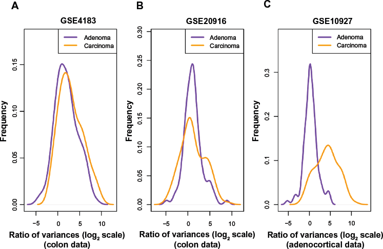Both adenoma and cancer samples show higher variability than normals (region to the right of x = 0), while cancer samples show higher hypervariability than adenomas. This suggests that hypervariability is a stable marker between experimental datasets and that specific selection of hypervariable genes across cancer types and the anti-profile method can be extended to model tumor progression. While a global Kolmogorov–Smirnov test for differences between the two distributions is not significant, further experiments with anti-profile scoring demonstrate that these probesets can be useful for differentiating between adenoma and cancer samples (see below).

Figure 1

Among probes that exhibit higher variability among cancers than among normals, the degree of hypervariability observed is related to the level of progression. (A) Distribution of variance ratio statistic $(\log_{2} [σ_{t u m o r}^{2} \div σ_{n o r m a l}^{2}])$ for colon dataset (Gyorffy et al; GSE4183) from anti-profile computed using another colon dataset (Skrzypczak et al; GSE20916). (B) Distribution of variance ratio statistic for Skrzypczak et al colon dataset from anti-profile computed using Gyorffy et al colon dataset. (C) Distribution of variance ratio statistic for adrenocortical data (Giordano et al; GSE10927) for universal anti-profile probesets.

Next, we performed an analysis using the universal anti-profile signature computed in Ref.12 We obtained an adrenocortical microarray dataset²⁰ containing normal, adenoma, and cancer samples. For the most hypervariable 100 probesets from the universal anti-profile, we plotted the distribution of variance of cancer/adenoma samples to variance of normal samples ratio (Fig. 1C). The same observations as before could be seen: a majority of these probesets show greater variability among cancer and adenoma samples than among normal samples, and this degree of variability is higher among cancer samples in comparison with adenoma samples (A Kolmogorov–Smirnov test between the two distributions with the alternative hypothesis being that the distribution for adenoma samples is less than that of cancer samples yields P = 1). This extends the suggestion of our hypothesis regarding hypervariability and tumor progression level to the universal anti-profile signature.

In the next stage of our experiments, we applied the anti-profile scoring method. As discussed in Ref. 12, the anti-profile scoring method counts the number of hypervariable probesets for which the expression of tumor samples lies beyond the normal region of expression. It has been shown to be an effective measurement in differentiating between tumor samples and normal samples, and our aim was to apply the same scoring method for differentiating between different stages of tumor progression. With the two colon-cancer datasets used to derive colon-cancer anti-profiles, we used the hypervariable probesets and the normal regions of expression for probesets derived from one dataset to calculate anti-profile scores for the normal, adenoma and cancer samples in the other dataset. The distribution of these scores are plotted in Figure 2A and B: for both datasets, the average anti-profile score increases from the normal group to the adenoma group to the cancer group: for the first dataset,¹⁷ the mean scores for these groups are 18.88, 27.93, and 35.33, respectively, and for the second dataset,¹⁸ the respective mean scores are 32.2, 51.4, and 58.9. 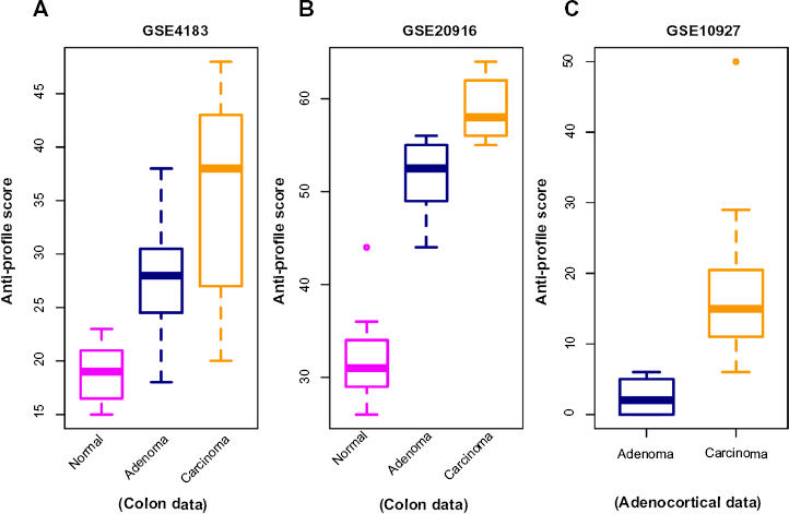Comparing the adenoma scores against the cancer scores yields an area under the receiver operating characteristic (ROC) curve (AUC) of 0.711 and a P-value of 0.05 from the Wilcoxon rank-sum test for the first dataset; the same comparison for the second dataset yields an AUC value of 0.97 and a P-value <10^-3 from the Wilcoxon rank-sum test.

Figure 2

Anti-profile scores calculated for tumors and normals. (A) Anti-profile scores for colon dataset (Gyorffy et al) from anti-profile computed using another colon dataset (Skrzypczak et al); carcinoma vs. adenoma AUC = 0.711 and Wilcoxon rank-sum test P-value = 0.05. (B) Anti-profile scores for Skrzypczak et al colon dataset from anti-profile computed using Gyorffy et al colon dataset; carcinoma vs. adenoma AUC = 0.97 and Wilcoxon rank-sum test P-value is <10^-3. (C) Anti-profile scores for adrenocortical data (Giordano et al) from universal anti-profile probesets; AUC = 0.997 and Wilcoxon rank-sum test P-value is <10^-4.

Similarly, we applied the anti-profile scoring method for the adrenocortical dataset with the universal anti-profile probesets (Fig. 2C). The cancer samples have higher anti-profile scores than the adenoma samples: the mean anti-profile scores are 2.5 and 16.84 for the adenoma and cancer groups, respectively. The comparison of the two score groups gives an AUC value of 0.997 and a Wilcoxon rank-sum test P-value of <10^-4. In addition, we also performed the same experiment on 10 follicular thyroid adenomas and 13 follicular thyroid carcinomas obtained from GSE27155,²¹ where we used the 100 most hypervariable probes from a universal anti-profile signature for the GPL96 platform (see the Application to Breast Cancer section). This provided an AUC of 0.808 and a Wilcoxon rank-sum test P-value of 0.01. However, only four normal samples were available in this dataset, thus limiting the confidence in the experimental result.

Anti-Profiles Based on DNA Methylation Also Capture Tumor Progression

DNA methylation is one of the primary epigenetic mechanisms for gene regulation, and is believed to play a particularly important role in cancer.²² High levels of methylation in promoter regions are usually associated with low transcription.^23,24 Abnormal methylation patterns have been observed in cancer, with loss of sharply methylation levels (in comparison with normal methylation levels) in regions associated with tissue differentiation,^19,25 and is associated with increased hypervariability in gene expression across multiple solid tumor types.²⁵ Given these observations, we expected that the anti-profile method would be applicable to methylation measurements from samples through cancer progression.

We applied the anti-profile scoring method to DNA methylation data from thyroid and colon samples,¹⁹ where for each tissue type, normal, adenoma and cancer samples were available. Using 384 probesets available in their custom Illumina methylation array data, for each cancer type, we used the normal samples to define the normal regions of methylation and calculated anti-profile scores by summing the number of features that fell outside the normal methylation region for each cancer sample.

Figure 3 shows the distribution of adenoma and carcinoma samples against normal samples on a principal component plot, showing the presence of the hypervariability pattern in methylation data: the normal samples cluster tightly, while the adenomas show some dispersion and the carcinomas show even greater dispersion. Since these behaviors are present for both colon and thyroid data, it again reinforces our notion that the anti-profile approach has wide application for classification in cancer.

Figure 3

Anti-profiles applied to methylation data: first two principal components of (A) thyroid methylation data and (B) colon methylation data.

Supplementary Figure 1 shows the results obtained with the anti-profile scores. As with the gene expression data, the methylation data also show that adenomas tend to have lower anti-profile scores than the carcinomas: for the thyroid tumors, the median anti-profile score for the adenoma class is 10, while for the carcinoma class is 17, and for the colon tumors, the median score for the adenoma class is 75.5, while for the carcinoma class is 121.5.

We also obtained data from a multiple solid tumor methylation study based on the Illumina HumanMethylation450 beadarray.²⁵ This dataset contains DNA methylation levels for normal, adenoma, and cancer samples comprised of thyroid, breast, colon, pancreas and lung tissues (see Supplementary Table 2).²⁵ Sample-specific methylation levels over CpG clusters were obtained as described in the Supplementary Methods section. To test the ability of anti-profile scoring to capture stable epigenetic marks across multiple tissue types, we followed a two-stage leave-one-tissue-out cross-validation procedure for each tissue type in the dataset (see Supplementary File), where feature selection for each tissue-specific anti-profile is based on consistent hypervariable methylation within common hypomethylation blocks of the other tissues in the dataset and anti-profile construction is based only on the normal samples of the tissue. In this case, no tumor data for each tissue are used when constructing their anti-profile. We observed high separation in anti-profile score between adenoma and tumor in all tissues (Supplementary Fig. 2, Wilcoxon rank-sum test; colon, P = 0.018; thyroid, P = 0.068; pancreas, P = 0.011; and breast, P = 0.058) and AUC greater than 0.8 for all tissues except thyroid (colon, AUC = 0.816; thyroid, AUC = 0.682; pancreas, AUC = 0.840; and breast, AUC = 0.837).

Increased Expression Variability is Associated with Clinical Outcome in Colon, Lung, and Breast Cancer

Based on the observation that increased expression variability and anti-profile scores in probesets with hypervariable expression is associated with tumor progression, we hypothesized that it will also be associated with clinical outcomes for tumors: aggressive tumors exhibiting poor clinical outcome would be associated with increased hypervariability in these specific genes and vice versa.

Application to Colon Cancer

We first experimented with a colon-cancer anti-profile as discussed in the previous section. We obtained a microarray dataset of colon tumor samples supplied with survival information (indicating the relapse of a patient within a certain number of years).²⁶ Using the other colon-cancer microarray datasets used in the previous section,^17,18 we constructed a colon-cancer anti-profile using the normal and cancer samples, limiting the probesets to the colon-cancer hypervariable genes from Corrada Bravo, et al.¹² A set of 100 probesets with the highest variability among cancer samples with respect to normal samples was selected from this anti-profile. These probesets and the normal regions of expression calculated for them using the normal colon samples from the abovementioned datasets together constituted the colon-cancer anti-profile used.

We stratified the samples into high risk and low risk as follows: patients who relapsed within 1 year after diagnosis were classified as high risk and those who did not relapse within 1 year were classified as low risk. For the selected probesets, we calculated the distribution of variance of high-/low-risk samples to variance of normal samples ratio (Supplementary Fig. 3). The hypervariability of the colon-cancer anti-profile probesets is reflected in these results, given that the majority of the probesets have a log₂ variance ratio >0. We can also see that the high-risk samples exhibit slightly higher variability than the low-risk samples when compared against the normals, affirming that the hypervariability observation extends to tumor prognosis as well.

Further, we calculated anti-profile scores for the colon tumor samples. Since the high-risk and low-risk grouping is not a well-defined classification, only tentatively captures tumor progression, we used Kaplan–Meier survival curves to measure the effectiveness of the anti-profile scores. We ordered the tumor samples according to the anti-profile score and stratified them to three equal- sized groups and observed the rate of survival in each group using Kaplan–Meier curves. This demonstrated that the anti-profile scores clearly correlate with the prognosis of the tumors, with higher anti-profile scores showing higher chances of relapse and vice versa (Fig. 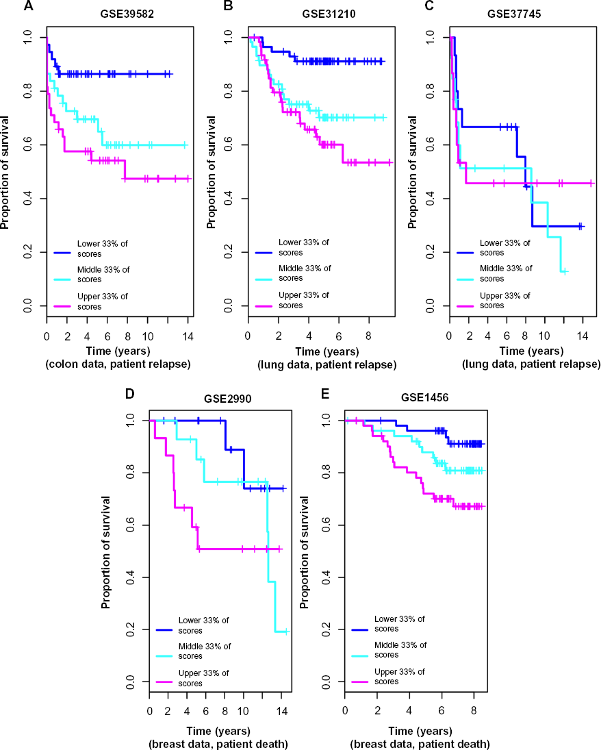4A; log-rank test score 9.452, P-value 0.008). We also noticed that the high-risk samples have a higher score on average than the low-risk samples (Supplementary Fig. 3): mean anti-profile scores for low-risk and high-risk groups are 41.85 and 48.87, respectively (Wilcoxon rank-sum test P-value is 0.0078 between the two groups).

Figure 4

Anti-profile scores correspond to tumor prognosis: (A) Kaplan–Meier survival curves for colon tumor samples ranked by anti-profile scores are grouped into three equal-sized groups; log-rank test score 9.452, P-value 0.008. (B) Survival curves for the first lung dataset (Okayama et al) – samples ranked by anti-profile scores are grouped to three equal-sized groups; log-rank test score 15.44, P-value <10^-4. (C) Survival curves fort the second lung dataset (Botling et al); log-rank test score 0.611, P-value 0.73. (D) Survival curves for the first breast dataset (Sotiriou et al); log-rank test score 3.971, P-value 0.137. (E) Survival curves for the second breast dataset (Pawitan et al); log-rank test score 10.467, P-value 0.005.

Application to Lung Cancer

Next, we applied the anti-profile method to analyze lung cancer survival. Here we tested the universal anti-profile from Corrada Bravo, et al.¹² with two microarray lung cancer datasets containing patient survival information based on patient relapse, the primary dataset containing both normal and tumor samples²⁷ and the secondary dataset containing only tumor samples.²⁸

As with the colon dataset, we stratified the samples into high risk and low risk based on patient relapse within five years. For the universal anti-profile probesets, we plotted the distribution of variance of high- and low-risk samples to variance of normal samples ratio (Supplementary Fig. 4). The majority of the universal anti-profile probesets show higher variability among the tumor samples than the normal samples, indicating that the universal anti-profile manages to capture the hypervariability property of these datasets.

We used normal lung samples to calculate anti-profile scores for the tumor samples for both datasets. Ordering the tumor samples by anti-profile score, for each dataset, we stratified them to three equal-sized groups and plotted Kaplan–Meier survival curves (Fig. 4B). For the first dataset, the tumor samples with the highest anti-profile scores show greatest relapse among the three groups, while the tumor samples with the lowest scores show the least relapse (log-rank statistic for the first dataset 15.44, P-value <10^-3). For the second dataset, we obtained a log-rank statistic 0.611 and a P-value 0.73 from the same procedure. The distribution of the scores for the high-risk and low-risk samples (Supplementary Fig. 5) indicates that for both datasets, the low-risk samples have lower antiprofile scores and vice versa (for the first dataset, the mean scores for low-risk and high-risk groups are, respectively, 14.32 and 19.81 with a Wilcoxon rank-sum test P-value of <10^-3; for the second dataset, the mean scores for low-risk and high-risk groups are, respectively, 31.64 and 33.32 with a Wilcoxon rank-sum test P-value of 0.58).

Figure 5

Anti-profiles applied to Cox proportional hazard models for survival prediction: Cox proportional hazard models with significant clinical covariates and anti-profiles were used to predict patient survival at 5 years for the second breast caner dataset (Pawitan et al) with (A) patient death and (B) patient relapse. The plots show accuracy of prediction calculated for 100 training and testing subsets randomly selected.

The results obtained for the second lung dataset did not show as much separation in the Kaplan–Meier survival curves when sorted into three groups. Comparing the generalized normalized unscaled standard error (GNUSE) values, a standard metric of microarray quality,²⁹ to compare the quality of the microarray data for the two lung cancer datasets (Supplementary Fig. 6), we noticed that this second dataset has a higher GNUSE value distribution in comparison to the first dataset, which might explain the poor performance. However, stratifying the samples as top 50% of scores and lower 50% of scores did show some separation of the two groups in terms of survival (log-rank statistic 1.418, P-value 0.22). The survival curves show the expected survival difference between the groups for the first 8 years, suggesting that the prognosis predicted by the anti-profile scores may become less relevant over time. In addition with increasing age, there is increased possibility that the health of a patient may deteriorate more aggressively.

The first dataset also contained information about death of patients. A similar analysis as before with patient death instead of relapse showed a log-rank statistic of 8.342 with P-value 0.015 when the samples were ranked by anti-profile scores and stratified to two groups (Supplementary Fig. 7).

These results demonstrate that the universal anti-profile probesets can be used to model the hypervariability in lung microarray data and further validate the use of using deviation from normal samples as a measurement of tumor prognosis.

Application to Breast Cancer

We next applied the methodology to breast cancer microarray data on Affymetrix Human Genome U133A platform (GPL96). Since the universal anti-profile signature had been derived from Affymetrix Human Genome U133 Plus 2.0 (GPL570) microarray data, we used a number of publicly available GPL96 platform cancer and normal samples (1207 cancer samples and 773 normal samples) of multiple tissue types to recalculate an anti-profile signature for the GPL96 platform (see the Methods section). We used the most significant 100 probesets from this signature for our breast cancer anti-profile experiments.

After obtaining two publicly available breast cancer microarray datasets,^30,31 we selected lymph node negative and estrogen receptor (ER) positive samples and verified that these probesets were able to capture the hypervariability of cancer samples (Supplementary Fig. 8). Since relapse information was not available for majority of the samples, we used death within 5 years as our criteria for obtaining a high-risk-low-risk classification.

We collected breast normal samples from publicly available datasets and calculated anti-profile scores for the two datasets. We drew Kaplan–Meier survival curves by ranking the samples by score and grouping them into three equal-sized classes (Fig. 4C). Similar to our observation with colon and lung cancer data, the anti-profile scores showed a correlation with survival of patients (log-rank statistic for the first dataset 3.971, P-value 0.137; log-rank statistic for the second dataset 10.467, P-value 0.005). The distribution of the scores for the high-risk and low-risk samples (Supplementary Fig. 9) demonstrates that high-risk samples have higher scores on average, and vice versa (for the first dataset, the mean scores for low-risk and high-risk groups are, respectively, 10.13 and 17.12 with a Wilcoxon rank-sum test P-value of 0.0061; for the second dataset, the mean scores for low-risk and high-risk groups are, respectively, 11.41 and 16.91 with a Wilcoxon rank-sum test P-value <10^-3).

The second breast dataset also contained information about patient relapse. Performing a similar analysis using relapse instead of death provided a log-rank statistic of 10.755 (P-value 0.004) when the samples were grouped by anti-profile score (Supplementary Fig. 10).

In addition, Supplementary Figure 11 shows similar results obtained for the third breast cancer dataset with patient death information. With only nine deaths being recorded, our method of stratifying samples into high-risk and low-risk classes was not appropriate for this dataset. However, we observed a trend of samples with high anti-profile scores exhibiting a higher rate of relapse and vice versa, as with the other datasets.

In summary, these results obtained for lung and breast cancer data further show the utility of the anti-profile approach as a robust and effective method for modeling tumor prognosis and validate our hypothesis that deviation from the normal group can be considered a measure of the risk level associated with a tumor.

Anti-Profile Approach is More Stable than Standard Classification Methods

We compared the anti-profile method with PAM using lung cancer data. For this, using the high-risk and low-risk stratification of samples previously described, we constructed a binary classification problem between low and high risk, and trained the PAM classifier on one dataset and tested the classifier on the other dataset. We used cross-validation on the training dataset to determine the threshold parameter that minimizes the misclassification error on the training data. The same experiment was performed between the two breast cancer datasets, and also, the two colon-cancer datasets used in our analysis were based on tumor progression (here the adenoma/carcinoma status was used as the binary stratification). The posterior probabilities obtained for the testing dataset were used to calculate AUC values and Wilcoxon rank-sum test P-values.

To compare against this, we applied the anti-profile method to the same training and testing dataset pairs. For each tissue type, we used normal samples and the tumor samples of one dataset to select probesets and calculate anti-profile scores for the other dataset. A comparison of these results can be seen in Table 1.

Table 1.

Comparison of prediction results obtained using the anti-profile scoring method and PAM. For each tissue type of lung, breast, and colon, two datasets with tumor samples were obtained and both the anti-profile method and the PAM model were fitted on one dataset and tested on the other dataset. For a binary stratification of samples by risk level, AUC values and the p-values from the Wilcoxon rank-sum test were calculated from the decision values resulting from each method. Datasets used were Lung1(GSE31210), Lung2(GSE37745), Breast1(GSE2990), Breast2(GSE1456), Colon1(GSE4183), and Colon2(GSE15960).

TESTED	TRAINING	ANTI-PROFILE SCORE		PAM
DATASET	DATASET	AUC	WILCOXON P-VALUE	AUC	WILCOXON P-VALUE
Lung1	Lung2	0.739	0.00002	0.663	0.003
Lung2	Lung1	0.44	0.571	0.5	1
Breast1	Breast2	0.712	0.08	0.641	0.25
Breast2	Breast1	0.707	0.0021	0.657	0.01
Colon1	Colon2	0.711	0.05	0.253	0.02
Colon2	Colon1	0.97	0.00042	0.87	0.003

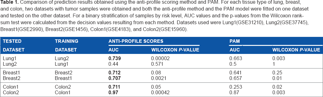
From the comparison of AUCs and the Wilcoxon rank-sum test P-values, we see that while the shrunken centroid classifier performed at a similar level with the one of the breast cancer datasets, it performed much poorly with the other datasets. Particularly with the lung cancer data, the PAM classifications failed to distinguish the high-risk and low-risk samples of the testing data. These results show that taking into account the stochastic hypervariability of cancers with regard to normals can produce more stable classifiers when building predictors across datasets.

Anti-Profile Approach may be used for Prognostic Prediction

To further examine the prognostic ability of the anti-profile score, we used the anti-profile scores as a covariate for modeling patient survival for some of the datasets. We obtained clinical covariates for the microarray datasets when publicly available and fitted each covariate separately to a Cox proportional hazards model to ascertain their prognostic significance. The Cox proportional hazards model is a widely used statistical model for assessing censored survival information.³² It provides a way for modeling the effect of a particular factor (such as age, severity of disease, etc) on the time taken by a patient to relapse (from the time of entering the clinical trial) or the time at which a patient dies. Here we treated the anti-profile score in the same manner as the other clinical factors.

For the first lung cancer dataset,²⁷ we tested age, sex, smoking status, and pathological stage. After fitting each covariate individually to a Cox proportional hazards model (assuming constant covariates) with patient relapse information, only pathological stage provided a P-value <0.05 from a Wald test. In addition, we also fitted the anti-profile score as a covariate, which also yielded P-value <0.05. Using patient death information instead of relapse, once again both pathological stage and anti-profile score showed significant association with survival (Wald test P < 0.05).

For the second breast cancer dataset,³¹ we tested pathological stage and subtype (Basal, ERBB2, Luminal A, Luminal B, Normal Like) for prognostic relevance with relapse and found that only pathological stage was significant when fitted to a Cox model (Wald test P < 0.05). The anti-profile scores provided P-value <0.05 as well. Using patient death information instead of survival produced similar results with pathological stage and anti-profile score, both showing prognostic significance when fitted independently (Wald test P < 0.05).

For the colon-cancer dataset with survival information (patient relapse),²⁶ we tested age, pathological stage, chemotherapy (treatment or lack of it), and location (distal vs. proximal). Pathological stage and chemotherapy status proved to be significant (Wald test P < 0.05, with pathological stage yielding P < 10^-5) when fitted independently to a Cox model. The anti-profile scores proved to be significant as well (P < 0.05).

For these datasets, we also tested the predictive ability of a Cox model fitted with the covariates selected above by predicting whether a given patient would live up to a given time t (we used t = 5 years). For this, we predicted the survival curve for that patient using a model fitted with a training set and compared the predicted survival curve to the rate of survival for the training group patients who did not survive at time t against training group patients who did survive up to time t. The dataset is split randomly into training (70%) and testing (30%) sets, and three Cox models are fitted to the training data: (a) a model with only selected clinical covariates, (b) a model with only anti-profile scores, and (c) a model with both clinical covariates and the anti-profile scores. For each model, the mean survival at time t is calculated for training set patients surviving and not-surviving at that time point. For each patient in the testing set, the predicted survival probability at time t is compared to the surviving group mean and not-surviving group mean, and the closest group is chosen to predict whether the patient will survive or not. These predictions are compared to actual survival to calculate an accuracy rate (patients censored by the time t are not used for the calculation). This process is repeated for a 100 training and testing subsets created from the main dataset, and the distribution of accuracy values was plotted.

For the second breast cancer dataset,³¹ a Cox model fitted with the pathological stage proved to be less accurate than a model fitted with the anti-profile score (Fig. 5A) for predicting patient death at 5 years. The mean accuracy level for the model fitted with the pathological stage was 0.619, for a model fitted with the anti-profile score was 0.726, and for a model fitted with both covariates was 0.655. A Wilcoxon test between the results from the first and third models yielded P-value <0.005, showing that the anti-profile score can significantly increase predictive power of a model. A similar test based on patient relapse (Fig. 5B) showed that all three model choices performed at a similar accuracy level, with the anti-profile score-based model providing a slightly higher accuracy rate.

We used a similar experiment on the lung and colon-cancer datasets mentioned above, but found that adding anti-profile scores to survival models, including significant clinical covariates, did not improve their performance significantly (Supplementary Fig. 12).

Conclusions

Our aim has been to develop a robust and stable approach for classification of tumor samples. We have demonstrated that the anti-profile scoring method, which was initially applied for classification between tumor and normal samples, can be extended to classification between tumor samples as well. This method has the particular advantage that tumor samples are only used to select probesets, but given this, the anti-profile score is based strictly on normal tissue samples. The ability of the anti-profile score to successfully provide a ranking of tumor samples, which correspond to their risk of relapse (or death) and the robustness of the method across experimental datasets, demonstrates that the universal anti-profile signature provides a robust basis to develop feature selection methods for tumor prognosis and diagnosis-related microarray experiments. In addition, it confirms our hypothesis behind the extension of the anti-profile approach to tumor prognosis: the measurement of deviation from a set of normal samples, which are likely to be more cohesive, is a more stable and robust indicator of the risk level of a tumor sample as opposed to direct comparisons between the highly variable tumor samples.

High-throughput technologies for gene expression measurements, especially microarrays, have progressed to the point that the use of gene expression data to develop gene expression-based cancer signatures is quite common in cancer research.³³ However, despite a number of gene expression profile-based signatures being published and even commercially utilized, in many instances, the developed signature has performed inadequately under subsequent validations. Validations of such signatures should ideally be carried out on populations completely independent of the population selected for the derivation of the signature. Only a few gene signatures produced, such as the Amsterdam 76-gene signature,³⁴ have proven to be reliable for clinical use.

Heterogeneity among multiple types of tumors has been a well-known observation.¹¹ While the proliferating ability of tumor cells is a widely used principle behind many prognostic gene signatures, this is usually measured via a mean-shift-based differential expression measurement. However, Feinberg and Irizarry³⁵ demonstrate that increased variance in the genotype may increase fitness via increased variability of the phenotype, regardless of any significant change in the mean phenotype. This shifts the focus of measuring tumor heterogeneity from a mean shift to a variance shift.

As part of a comprehensive study of the colon-cancer methylome, the degree of hypervariability in DNA methylation between the adenoma and the cancer samples was observed to increase significantly.¹⁹ When projected to a lower dimensional space using PCA, the normal samples clustered tightly together with the cancer samples dispersed and the adenoma samples demonstrated an intermediate degree of variability and an intermediate distance to the normal cluster. Based on these findings, Bravo et al.¹² introduced anti-profiles as a stable method for screening multiple types of cancer. The principle underlying this model of cancer screening is that certain genes will consistently show higher across-samples variability among cancer samples as compared with normal samples. In this study, these genes are identified and the hyper-variability is used to predict outcome, where the model is referred to as an anti-profile as it measures variation from normal behavior. The same study also demonstrated that the genes corresponding to expression hypervariability in cancer are also generally tissue-specific genes, an observation that is utilized to develop a universal anti-profile. Recent studies have looked at gene expression variability in the context of geneset and pathway discovery³⁶ and unsupervised construction of profiles in prostate cancer based on outlier analysis.³⁷

The anti-profile methods developed here are applications and extensions to the predictive setting of ideas in existing statistical methods developed to identify and model outliers in gene expression because of cancer,^38,39 and other extensions are in active development.⁴⁰ These ideas are increasingly used in the analysis of epigenetic data.^41,42 The general idea of using deviation from a stable class to classify between groups of anomalies is underdeveloped in the machine learning field, but should prove to be a fertile ground for the development of general methodology.⁴³

The results presented here confirm that an anomaly classification-based approach to gene expression and methylation-based experiments of tumor prognosis and diagnosis can be highly valuable. In summary, our work shows by application to lung cancer, breast cancer, colon-cancer and adrenocortical tumor gene expression datasets, and also to thyroid and colon methylation data, that the anti-profile approach does in fact produce models that are accurate, robust, and stable.

Author Contributions

Conceived and designed the experiments: HCB, WD. Analyzed the data: WD. Wrote the first draft of the manuscript: WD, HCB. Jointly developed the structure and arguments for the paper: HCB, WD. Both authors reviewed and approved of the final manuscript.

supplementary Materials

Supplementary Table 1.

A summary of the gene expression microarray datasets used.

Supplementary Table 2

A summary of the DNA methylation datasets used.

Supplementary Figure 1

Anti-profiles applied to methylation data: (A) Distribution of anti-profile scores for adenoma and carcinoma for thyroid tumor samples from methylation data (AUC = 0.784, Wilcoxon rank-sum P value < 10^-5); (B) Distribution of anti-profile scores for adenoma and carcinoma for colon tumor samples from methylation data (AUC = 0.717, Wilcoxon rank-sum P value = 0.093).

Supplementary Figure 2

Anti-profiles applied to Illumina Human Methylation 450 data: Distribution of anti-profile scores for adenoma and carcinoma for (A) Thyroid (B) Colon (C) Pancreas and (D) Breast tissue samples.

Supplementary Figure 3

Colon cancer survival analysis based on patient relapse: (A) Distribution of variance ratio statistic for high risk and low risk samples from colon dataset (Marisa et al.; GSE39582) from an anti-profile computed using another colon data. (B) Distribution of anti-profile scores among low risk and high risk samples; AUC = 0.684, Wlcoxon rank-sum test P-value = 0.0078.

Supplementary Figure 4

Lung cancer survival analysis based on relapse: (A) Distribution of variance ratio statistic for high risk and low risk samples from first lung dataset (Okayama et al.; GSE31210) for 100 universal anti-profile probests with the highest hyper-variability. (B) Distribution of variance ratio statistic for high risk and low risk samples from second lung dataset (Botling et al.; GSE37745) for 100 universal anti-profile probests with the highest hyper-variability.

Supplementary Figure 5

Lung cancer prognosis is related to the anti-profile score: (A) Anti-profile scores for first dataset (Okayama et al.) high and low risk samples from universal anti-profile probesets; AUC = 0.716, Wlcoxon rank-sum test P-value < 10^-3. (B) Anti-profile scores for second dataset (Botling et al.) high and low risk samples; AUC = 0.558, Wlcoxon rank-sum test P-value = 0.58.

Supplementary Figure 6

GNUSE value comparison: Distribution of generalized normalized unscaled standard error values for the two lung cancer datasets, GSE31210 (Okayama et al.), and GSE37745 (Botling et al.).

Supplementary Figure 7

Additional lung cancer survival results: (A) Kaplan–Meier survival curves based on patient death for first lung dataset (Okayama et al.); samples ranked by anti-profile scores are grouped to three equal sized groups; Logrank test score 8.342, P-value 0.015. (B) Distribution of same anti-profile scores for high and low risk classification based on patient death within 5 years; AUC = 0.685, Wlcoxon rank-sum test P-value 0.01.

Supplementary Figure 8

Breast cancer analysis based on patient death: (A) Distribution of variance ratio statistic for high risk and low risk samples from first breast dataset (Sotiriou et al.; GSE2990) for 100 universal anti-profile probests with the highest hyper-variability. (B) Distribution of variance ratio statistic for high risk and low risk samples from second breast dataset (Pawitan et al.; GSE1456) for 100 universal anti-profile probests with the highest hyper-variability.

Supplementary Figure 9

Breast cancer prognosis is related to the anti-profile score: (A) Anti-profile scores for first dataset (Sotiriou et al.) high and low risk samples from universal anti-profile probesets; AUC = 0.832, Wlcoxon rank-sum test P-value 0.0061. (B) Anti-profile scores for second dataset (Pawitan et al.) high and low risk samples; AUC = 0.743, Wlcoxon rank-sum test P-value < 10^-3.

Supplementary Figure 10

Additional breast cancer survival results: (A) Kaplan–Meier survival curves based on relapse for second breast cancer dataset (Pawitan et al.); samples ranked by anti-profile scores are grouped to three equal sized groups; Logrank test score 10.755, P-value 0.004. (B) Distribution of same anti-profile scores for high and low risk classification based on relapse within 5 years; AUC = 0.703, Wlcoxon rank-sum test P-value < 10^-3.

Supplementary Figure 11

Additional breast cancer survival results: (A) Kaplan–Meier survival curves based on patient death for an additional breast cancer dataset (Miller et al.; GSE3494); samples ranked by anti-profile scores are grouped to three equal sized groups; Logrank test score 0.696, P-value 0.706. (B) Anti-profile scores obtained for the third breast cancer dataset for a risk classification based on patient death or survival within 8 years (48 low risk and 6 high risk samples); AUC = 0.694, Wlcoxon rank-sum test P-value 0.1257. Our method of stratifying samples into risk groups was not well applicable for this dataset.

Supplementary Figure 12

Anti-profiles applied to Cox models for survival prediction: Cox proportional hazard models with significant clinical covariates and anti-profiles were used to predict patient survival at 5 years for (A) first lung cancer dataset (Okayama et al.) with patient relapse, (B) first lung cancer dataset with patient death, and (C) colon cancer dataset (Marisa et al.) with patient relapse. The plots show accuracy of prediction calculated for 100 training and testing subsets randomly selected. Model M0 only contains significant clinical covariates, model M1 contains only the anti-profile score, and model M2 contains both selected clinical covariates and the anti-profile score.

References

Tabár

, Fagerberg

C.J.

, Gad

. Reduction in mortality from breast cancer after mass screening with mammography: randomised trial from the breast cancer screening working group of the Swedish national board of health and welfare. Lancet. 1985; 325: 829–32.

Newcomb

P.A.

, Norfleet

R.G.

, Storer

B.E.

, Surawicz

T.S.

, Marcus

P.M.

Screening sigmoidoscopy and colorectal cancer mortality. J Natl Cancer Inst. 1992; 84: 1572–5.

Andriole

G.L.

, Crawford

E.D.

, Grubb

III . PLCO Project Team. Mortality results from a randomized prostate-cancer screening trial. N Engl J Med. 2009; 360: 1310–9.

Mandel

J.S.

, Bond

J.H.

, Church

T.R.

. Reducing mortality from colorectal cancer by screening for fecal occult blood. N Engl J Med. 1993; 328: 1365–71.

Walsh

J.M.

, Terdiman

J.P.

Colorectal cancer screening: scientific review. JAMA. 2003; 289: 1288–96.

Klabunde

C.N.

, Vernon

S.W.

, Nadel

M.R.

, Breen

, Seeff

L.C.

, Brown

M.L.

Barriers to colorectal cancer screening: a comparison of reports from primary care physicians and average-risk adults. Med Care. 2005; 43: 939–44.

Lerman

, Rimer

, Trock

, Balshem

, Engstrom

P.F.

Factors associated with repeat adherence to breast cancer screening. Prev Med. 1990; 19: 279–90.

Harewood

G.C.

, Wiersema

M.J.

, Melton

LJ.

III . A prospective, controlled assessment of factors influencing acceptance of screening colonoscopy. Am J Gastroenterol. 2002; 97: 3186–94.

Veer

L.J.

, Dai

, Van De Vijver

M.J.

. Gene expression profiling predicts clinical outcome of breast cancer. Nature. 2002; 415: 530–6.

10.

Gianni

, Zambetti

, Clark

. Gene expression profiles in paraffin-embedded core biopsy tissue predict response to chemotherapy in women with locally advanced breast cancer. J Clin Oncol. 2005; 23: 7265–77.

11.

Koscielny

Why most gene expression signatures of tumors have not been useful in the clinic. Sci Transl Med. 2010; 2: s2–14.

12.

Bravo

H.C.

, Pihur

, McCall

, Irizarry

, Leek

Gene expression anti-profiles as a basis for accurate universal cancer signatures. BMC Bioinformatics. 2012; 13: 272.

13.

McCall

M.N.

, Jaffee

H.A.

, Irizarry

R.A.

fRMA ST: frozen robust multiarray analysis for affymetrix exon and gene ST arrays. Bioinformatics. 2012; 28: 3153–54.

14.

McCall

M.N.

, Uppal

, Jaffee

H.A.

, Zilliox

M.J.

, Irizarry

R.A.

The gene expression barcode: leveraging public data repositories to begin cataloging the human and murine transcriptomes. Nucleic Acids Res. 2011; 39: 1011–5.

15.

Bravo

H.C.

, Irizarry

R.A.

, Leek

J.T.

antiProfiles: Implementation of Gene Expression Anti-Profiles. R package version 1.6.0. 2013

16.

Tibshirani

, Hastie

, Narasimhan

, Chu

Diagnosis of multiple cancer types by shrunken centroids of gene expression. Proc Natl Acad Sci U S A. 2002; 99: 6567–72.

17.

Gyorffy

, Molnar

, Lage

, Szallasi

, Eklund

A.C.

Evaluation of microarray preprocessing algorithms based on concordance with RT-PCR in clinical samples. PLoS One. 2009; 4: e5645.

18.

Skrzypczak

, Goryca

, Rubel

. Modeling oncogenic signaling in colon tumors by multidirectional analyses of microarray data directed for maximization of analytical reliability. PLoS One. 2010; 5: e13091.

19.

Hansen

K.D.

, Timp

, Bravo

H.C.

. Increased methylation variation in epigenetic domains across cancer types. Nat Genet. 2011; 43: 768–75.

20.

Giordano

T.J.

, Kuick

, Else

. Molecular classification and prognostication of adrenocortical tumors by transcriptome profiling. Clin Cancer Res. 2009; 15: 668–76.

21.

Giordano

T.J.

, Kuick

, Thomas

D.G.

. Molecular classification of papillary thyroid carcinoma: distinct BRAF, RAS, and RET/PTC mutation-specific gene expression profiles discovered by DNA microarray analysis. Oncogene. 2005; 24: 6646–56.

22.

Gal-Yam

E.N.

, Saito

, Egger

, Jones

P.A.

Cancer epigenetics: modifications, screening, and therapy. Annu Rev Med. 2008; 59: 267–80.

23.

Suzuki

M.M.

, Bird

DNA methylation landscapes: provocative insights from epigenomics. Nat Rev Genet. 2008; 9: 465–76.

24.

, Zhu

, Tian

. The DNA methylome of human peripheral blood mononuclear cells. PLoS Biol. 2010; 8: e1000533.

25.

Timp

, Bravo

H.C.

, McDonald

O.G.

. Large hypomethylated blocks as a universal defining epigenetic alteration in human solid tumors. Genome Med. 2014; 6: 61.

26.

Marisa

, de Reyniès

, Duval

. Gene expression classification of colon cancer into molecular subtypes: characterization, validation, and prognostic value. PLoS Med. 2013; 10: e1001453.

27.

Okayama

, Kohno

, Ishii

. Identification of genes upregulated in ALK-positive and EGFR/KRAS/ALK-negative lung adenocarcinomas. Cancer Res. 2012; 72: 100–11.

28.

Botling

, Edlund

, Lohr

. Biomarker discovery in non-small cell lung cancer: integrating gene expression profiling, meta-analysis, and tissue microarray validation. Clin Cancer Res. 2013; 19: 194–204.

29.

McCall

M.N.

, Murakami

P.N.

, Lukk

, Huber

, Irizarry

R.A.

Assessing affymetrix GeneChip microarray quality. BMC Bioinformatics. 2011; 12: 137.

30.

Pawitan

, Bjöhle

, Amler

. Gene expression profiling spares early breast cancer patients from adjuvant therapy: derived and validated in two population-based cohorts. Breast Cancer Res. 2005; 7: R953.

31.

Miller

L.D.

, Smeds

, George

. An expression signature for p53 status in human breast cancer predicts mutation status, transcriptional effects, and patient survival. Proc Natl Acad Sci USA. 2005; 102: 13550–5.

32.

Spruance

S.L.

, Reid

J.E.

, Grace

, Samore

Hazard ratio in clinical trials. Antimicrob Agents Chemother. 2004; 48: 2787–92.

33.

Subramanian

, Simon

Gene expression-based prognostic signatures in lung cancer: ready for clinical use?

J Natl Cancer Inst. 2010; 102: 464–74.

34.

Wang

, Klijn

J.G.

, Zhang

. Gene-expression profiles to predict distant metastasis of lymph-node-negative primary breast cancer. Lancet. 2005; 365: 671–9.

35.

Feinberg

A.P.

, Irizarry

R.A.

Stochastic epigenetic variation as a driving force of development, evolutionary adaptation, and disease. Proc Natl Acad Sci U S A. 2010; 107: 1757–64.

36.

Afsari

, Geman

, Fertig

E.J.

Learning dysregulated pathways in cancers from differential variability analysis. Cancer Inform. 2014; 13(suppl 5): 61–7.

37.

Ghosh

, Li

Unsupervised outlier profile analysis. Cancer Inform. 2014; 13: 25–33.

38.

MacDonald

J.W.

, Ghosh

COPA–cancer outlier profile analysis. Bioinformatics. 2006; 22: 2950–1.

39.

Tibshirani

, Hastie

Outlier sums for differential gene expression analysis. Biostatistics. 2007; 8: 2–8.

40.

Wang

, Taciroglu

, Maetschke

S.R.

, Nelson

C.C.

, Ragan

M.A.

, Davis

M.J.

mCOPA: analysis of heterogeneous features in cancer expression data. J Clin Bioinforma. 2012; 2: 22.

41.

Teschendorff

A.E.

, Jones

, Fiegl

. Epigenetic variability in cells of normal cytology is associated with the risk of future morphological transformation. Genome Med. 2012; 4: 24.

42.

Chambwe

, Kormaksson

, Geng

. Variability in DNA methylation defines novel epigenetic subgroups of DLBCL associated with different clinical outcomes. Blood. 2014; 123: 1699–708.

43.

Dinalankara

, Bravo

H.C.

Anomaly classification with the anti-profile support vector machine. arXiv org. 2013: 1301.3514.

Gene Expression Signatures Based on Variability can Robustly Predict Tumor Progression and Prognosis

Abstract

Keywords

Background

Methods

Results and Discussion

Gene Expression Anti-Profiles Capture Tumor Progression

Anti-Profiles Based on DNA Methylation Also Capture Tumor Progression

Increased Expression Variability is Associated with Clinical Outcome in Colon, Lung, and Breast Cancer

Application to Colon Cancer

Application to Lung Cancer

Application to Breast Cancer

Anti-Profile Approach is More Stable than Standard Classification Methods

Anti-Profile Approach may be used for Prognostic Prediction

Conclusions

Author Contributions

supplementary Materials

Supplementary Table 1.

Supplementary Table 2

Supplementary Figure 1

Supplementary Figure 2

Supplementary Figure 3

Supplementary Figure 4

Supplementary Figure 5

Supplementary Figure 6

Supplementary Figure 7

Supplementary Figure 8

Supplementary Figure 9

Supplementary Figure 10

Supplementary Figure 11

Supplementary Figure 12

References