Web Tool for Estimating the Cancer Hazard Rates in Aging

Abstract

A computational approach for estimating the overall, population, and individual cancer hazard rates was developed. The population rates characterize a risk of getting cancer of a specific site/type, occurring within an age-specific group of individuals from a specified population during a distinct time period. The individual rates characterize an analogous risk but only for the individuals susceptible to cancer. The approach uses a novel regularization and anchoring technique to solve an identifiability problem that occurs while determining the age, period, and cohort (APC) effects. These effects are used to estimate the overall rate, and to estimate the population and individual cancer hazard rates. To estimate the APC effects, as well as the population and individual rates, a new web-based computing tool, called the CancerHazard@Age , was developed. The tool uses data on the past and current history of cancer incidences collected during a long time period from the surveillance databases. The utility of the tool was demonstrated using data on the female lung cancers diagnosed during 1975–2009 in nine geographic areas within the USA. The developed tool can be applied equally well to process data on other cancer sites. The data obtained by this tool can be used to develop novel carcinogenic models and strategies for cancer prevention and treatment, as well as to project future cancer burden.

Introduction

The concept of the population cancer hazard rates in aging is tightly connected with the concept of the age-specific incidence rates that are characterized by a number of new cancers of a specific site/type, occurring within an age-specific group of individuals from a specified population during a distinct time period.^1–6 The population hazard rates in aging, which we will call the population hazard rates (or just population rates), are determined by a correction of the age-specific incidence rates on the age, period, and cohort (APC) effects (see Refs. 5–7 and below).

Recently, ⁵ a novel concept, the individual hazard rates in aging (shortly, individual rates), was introduced. This concept assumes that only a small fraction (pool) of individuals in the population is susceptible to cancer, while the rest of the population (a large fraction) is resistant to cancer. The individual rates characterize the risk of getting cancer for the age-specific group of individuals who are susceptible to cancer and will get cancer in their lifetime.

The main obstacle to the wide use of the population and individual rates in cancer research is the absence of a simple computational approach and a freely available computerized tool for their estimation. The present work is aimed at filling this gap.

The APC effects are more typical for adult rather than for childhood cancers. This is because the occurrence of adult cancers is often associated with lifestyle and environmental risk factors, while the occurrence of childhood cancers is often linked to genetic abnormalities. Since the adult cancers are usually diagnosed at the ages of 20 and older, analysis of the occurrence of these cancers is performed using cancer-related data on people in that age group.

In cancer epidemiology, the APC effects are often estimated in the frame of the log-linear age–period–cohort (LLAPC) model. While using this model, however, the identifiability problem arises. To solve this problem, the use of additional assumptions or specific estimable functions is needed (see Refs. 8–13 and references therein). Recently, in Ref. 9, a novel estimable function, called the fitted age-at-onset curve, was introduced and used to develop the AgePeriodCohort web tool (http://analysistools.nci.nih.gov/apc/). ¹⁰

In the present work, we expanded the traditional approach,^11–13 in which (within a set of the unknown parameters required for estimating the APC effects) four redundant parameters are equated to zero. In our approach, we set only three parameters to zero and determined an optimal value of the fourth parameter by an assumption that the effects of the adjacent cohorts are close. ⁷ To the best of our knowledge, this is the mildest assumption used so far to solve the APC problem.

Based on the approach ⁷ and using a simple regularization and anchoring technique, we developed a novel computational framework to estimate the APC effects, the population and individual hazard rates of cancer development in aging, and the overall cumulative hazard rate (or shortly the overall rate). In this framework, the population hazard rates are estimated by correcting the observed age-specific incidence rates of cancer on the APC effects. After that, the overall rate and the individual rates are determined.

The proposed computational framework was implemented in a new, stand-alone web tool, called CancerHazard@Age. This tool is freely available at http://registry.unmc.edu/CHA/.

The performance of CancerHazard@Age was demonstrated using data on the female lung cancers diagnosed in 1975–2009 in nine geographic areas within the USA.

Materials and Methods

Mathematical Methods.

Age-Specific Incidence Rates.

The age-specific incidence rates can be determined as a ratio of the number of cancer cases, O_i,j, divided by the total person-years at risk, P_i,j, in equal age intervals. P_i,j is determined as the size of a population, Pop _i,j , multiplied by the “width (in years) of the time periods of observations, δ. For better accountability and to avoid the use of small decimal numbers, the age-specific incidence rates of cancer are expressed as a number of new cancer cases per 100,000 person-years in five-year age groups.

APC Analysis.

In the frame of the LLAPC model, the APC analysis is performed using the following system of conditional equations:

$$\begin{array}{r}{Y}_{i,j}=\mu +{\alpha }_i+{\beta }_j+{\gamma }_k,\hspace{0.17em}\hspace{0.17em}\left(i=1,\mathrm{\dots },n\right)\hspace{0.17em}\hspace{0.17em}\left(j=1,\mathrm{\dots },m\right)\\ \left(k=j-i+n=1,\mathrm{\dots },l\right)\end{array}$$

(1)

In the system (1):

$$Y_{i,j}=\ln \left(I_{i,j}\right)=\ln \left(\frac{O_{i,j}}{P_{i,j}}\right),\hspace{0.17em}\hspace{0.17em}(i=1,\mathrm{\dots },n)\hspace{0.17em}\hspace{0.17em}(j=1,\mathrm{\dots },m)$$

(2) where Y_i,j is a logarithm of the incidence rate, I_i,j; O_i,j is the number of cancer occurrences; and P_i,j is the person-years at risk. In the system (1), α _i is the age (A) effect; β _j is the time-period (P) effect; γ _k is the birth cohort (C) effect; and μ is a constant, called the intercept. ² The age intervals are indexed as (i = 1, …, n); the time-period intervals of cancer occurrences are indexed as (j = 1, …, m); the birth cohort intervals of cancer occurrences are indexed as (k = j − 1 + n = 1, …, l); and n, m, and l are numbers of the age intervals, time periods, and birth cohorts, which are indexed correspondingly. The matrixes, O _i,j and P _i,j , are obtained from observations. The APC effects and the intercept are estimated by solving the system (1).

In the model used, Y_i,j are taken with weights (w_i,j), which are inversely proportional to their sampling variances, SE ² (Y_i,j). In this case, according to Ref. 7:

$$w_{i,j}=O_{i,j},\hspace{0.17em}\hspace{0.17em}(i=1,\mathrm{\dots },n)\hspace{0.17em}\hspace{0.17em}(j=1,\mathrm{\dots },m)$$

(3)

The problem is to determine from the system of the n × m conditional equations (1) with weights (3) the following: (i) the n estimates of the A effects, ${\alpha }_i^{*}$ ; (ii) the m estimates of the P effects, ${\beta }_j^{*}$ ; (iii) the l estimates of the C effects, ${\gamma }_i^{*}$ ; and (iv) the intercept, μ*. Here and below the asterisks sign, ^*, designates estimates.

The system (1) cannot be solved directly by methods of multiple linear regressions. This is because the design matrix of the system (1) is rank deficient because of a linear interrelation of the APC effects. Consequently, the APC effects cannot be uniquely and simultaneously estimated (multiple estimators of these effects provide similar solutions). In this work, to solve this identifiability problem, we used the heuristic approach proposed in Ref. 7. We implemented this approach in the computational framework, which we used for developing the CancerHazard@Age tool (see Results and Discussion).

Data Preparation.

The CancerHazard@Age tool was tested using data on the female lung cancers diagnosed in 1975–2009 in San Francisco-Oakland SMSA, Connecticut, Detroit (Metropolitan), Hawaii, Iowa, New Mexico, Seattle (Puget Sound), Utah, and Atlanta (Metropolitan) areas. Data on lung cancer cases were obtained from the database. ¹⁴ Data on the female populations were obtained from the databases.^15,16 Data on the female lung cancers and on the sizes of the female populations were extracted by SEER^*Stat 8.1.5 software, ¹⁷ and used to create the case and population matrixes utilized for testing the CancerHazard@Age tool.

Obtaining Data for the Case Matrix.

Initially, from the database, ¹⁴ we selected and saved a column with 19 numbers of histologically confirmed female lung cancers, diagnosed during the 1975–1979 time period in 19 age intervals (0, 1–4, 5–9, …; 80–84, and 85+). Then, we extended this column by splitting the number of cases in the 85+ age interval into the number of the female lung cancers in the 85–89, 90–94, 95–99, and 100+ age intervals. To do this, we determined a number of the cancers in the 85–89, 90–94, 95–99, and 100+ age intervals. Thus, we obtained a column with the numbers of the histologically confirmed female lung cancers diagnosed in 22 age intervals (0, 1–4, 5–9, 95–99, and 100+ years) during the 1975–1979 time period. Analogously, we determined columns with 22 numbers of the female lung cancers diagnosed during the 1980–1984, …, 2005–2009 time periods.

Overall, we obtained seven columns with 22 numbers of the histologically confirmed female cancers diagnosed in 22 age intervals (0, 1–4, 5–9, …, 95–99, and 100+) and in seven time periods (1975–1979, …, 2005–2009). Then, we concatenated (joined) these seven columns into one 22 × 7 matrix. Finally, we omitted six age intervals (0, 1–4, 5–9, 10–14, 15–19, and 100+) in which the numbers of lung cancers were small (less than 10). Thus, we truncated the 22 × 7 matrix to the 16 × 7 matrix, presenting the number of the female lung cancers diagnosed in 16 age intervals (20–24, …, 95–99) in seven time periods (1975–1979, …, 2005–2009). This truncated matrix was used for testing the CancerHazard@Age.

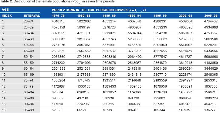
Obtaining Data for the Population Matrix.

Using the database, ¹⁵ we created columns with 19 numbers showing the female populations in 19 age intervals (0, 1–4, 5–9, …, 80–84, and 85+ years) in the 1975–1979 time period. We also created analogous columns showing the female populations in the 1980–1984, 1985–1989, 1990–1994, and 1995–1999 time periods. Using the database, ¹⁶ we created columns showing the female populations in 22 age intervals (0, 1–4, 5–9, …, 95–99, and 100+ years) in the 2000–2004 and the 2005–2009 time periods.

To estimate the sizes of the female populations in the 85–89, 90–94, 95–99, and 100+ age intervals in the first five time periods considered (ie, 1975–1979, …, 1995–1999), we proportionally split the sizes of the female populations in the 85+ age interval based on the female populations in the 85–89, 90–94, 95–99, and 100+ age intervals. The proportions were estimated from the female populations observed within 2000–2009 in the 85–89, 90–94, 95–99, and 100+ age intervals. Thus, for all seven time periods, we obtained seven columns with the female populations in 22 age intervals (0, 1–4, 5–9, …, 95–99, and 100+).

Finally, we concatenated the obtained columns into one 22 × 7 matrix. This matrix presents the female populations in 22 age intervals (0–4, 5–9, …, 95–99, 100+) for the consecutive seven five-year time periods (1975–1979, 1980–1984, 1985–1989, 1990–1994, 1995–1999, 2000–2004, and 2005–2009). Finally, by omitting the female populations in six age intervals (0, 1–4, 5–9, 10–14, 15–19, and 100+), we truncated the obtained 22 × 7 population matrix to the 16 × 7 matrix. This was done to have the same dimensions for the case and population matrices.

Results and Discussion

Computational Framework.

We developed a three-step computational framework to estimate the population and individual hazard rates. In the first step, the APC effects and the intercept were estimated. In the second step, using these estimates, the population hazard rates were determined. Finally, in the third step, from the determined population hazard rates, the individual hazard rates were estimated. A more detailed description of this framework is presented below.

Step 1. To determine the APC effects, the following anchoring procedure is performed. Three parameters ( $({\alpha }_{i_0}=0,\hspace{0.17em}{\beta }_{j_0}=0,{\gamma }_{k_0}=0)$ ) are set to zero. The proposed framework offers two possible ways of choosing the i₀, j₀, and k₀ indexes to anchor the A, P, and C effects, correspondingly.

One way, which we called manual anchoring, is in using the appropriate, up-front given integer numbers as the i₀ and j₀ indexes. These numbers can be taken from the following two sets of numbers: {1, …, n} and {3, …, m}, where n is the number of the considered age intervals and m is the number of the time periods. The k₀ index is determined as k₀ = j₀ − i₀ + n. The choice of these indexes depends on the used observed data and on how the APC effects (to be determined) will be further used.

The other way, which we called an automatic anchoring, is to algorithmically determine the i₀, j₀, and k₀ indexes. This determination starts with choosing the j₀ index that presents a median time period. Specifically, when the number of time periods, m, is odd, the central index is used as the anchor period index, j₀. When m is even, the upper of the two median indexes is used as j₀. After getting j₀, the index, i₀, for which the corresponding equation in system (1) for the given j₀ has a maximum weight (ie, $O_{i_0,j_0}=\max$ ) is chosen as the anchor age index. Finally, k₀ is determined as k₀ = j₀ − i₀ + n.

By setting ${\alpha }_{i_0}=0$ , ${\beta }_{j_0}=0$ , ${\gamma }_{k_0}=0$ , the identifiability problem is reduced to the problem of determining one redundant parameter called the identification parameter. ⁷ In the proposed framework, the P effect, ${\beta }_{j_0-1}$ , designated by $\delta (\delta ={\beta }_{j_0-1})$ , is used as the identification parameter. By varying δ, a family of estimates of the APC effects is obtained. To get an optimal value of the identification parameter, a heuristic assumption that the effects of the adjacent cohorts are close is used. By this assumption, the optimal value of δ is numerically determined by minimizing (with respect to δ) the weighted average of the squared differences between the estimates of the adjacent C effects, ${({\gamma }_{k+1}^{*}-{\gamma }_k^{*})}^2$ . This optimization problem is formulated as follows ⁷ :

$$\frac{1}{{\sum }_{k=1}^{l=1}{W}_k}{\sum }_{k=1}^{l=1}{W}_k{({\gamma }_{k+1}^{*}-{\gamma }_k^{*})}^2\to {\min }_{\delta }$$

(4) where the weights, W_k, are reciprocals of the variances of the differences between estimates of the adjacent C effects, ( $({\gamma }_{k+1}^{*}-{\gamma }_k^{*})$ ). In the proposed framework, the optimal value of δ that gives the best solution of the system (1) is obtained by varying δ within the interval, [−0.5, 0.5], with the step equal to 0.001. This solution provides a unique set of estimates of the A, P, and C effects, ${\alpha }_i^{*},{\beta }_j^{*},{\gamma }_k^{*}$ , and the estimates of the intercept, μ^*, as well as the estimates of their standard errors, SE^*.

Step 2. The estimates of the population rates, $h_{U,i}^{*},$ , and their standard errors, SE* $\left(h_{U,i}^{*}\right)$ , in the successive age intervals i (i = 1, …, n) are determined by ${\alpha }_i^{*}$ , μ^*, SE^* $\left({\alpha }_i^{*}\right)$ , and SE^*(μ^*), estimated on the previous step, as follows ⁷ :

$$h_{U,i}^{*}=\exp \left({\mu }^{*}+{\alpha }_i^{*}\right)\hspace{0.17em}\left(i=1,\mathrm{\dots },n\right)$$

(5) and

$$S{E}^{*2}\left(h_{U,i}^{*}\right)=h_{U,i}^{*2}\left[S{E}^{*2}\left({\mu }^{*}\right)+S{E}^{*2}\left({\alpha }_i^{*}\right)\right]\hspace{0.17em}\hspace{0.17em}\left(i=1,\mathrm{\dots },n\right)$$

(6)

Step 3. The estimates of the individual rates, $h_i^{*}$ , and their standard errors, SE $\left(h_i^{*}\right)$ , are obtained by formulas (34)–(39) in Ref. 5.

Web-Based Computing Tool, CancerHazard@Age.

The proposed computational framework was incorporated into a computing tool, called the CancerHazard@Age , which is aimed at estimating the overall hazard rate, and the population and individual hazard rates of a specific cancer site/type. The tool is a two-tier web application. The business logic of this tool primarily lies within Java classes. The graphical user interface of the CancerHazard@Age is implemented as JavaServer Pages (JSP). The JAMA library (developed by the MathWorks and the National Institute of Standards and Technology) is used to perform the calculations, and the JFreeChart library (developed by the Object Refinery Limited) is utilized to build graphs. The input and output pages of the CancerHazard@Age tool are shown in Figures 1 and 2, correspondingly.

Figure 1.

Screen shot of the input page. The page shows values of the input data described in Section utility of the CancerHazard@Age.

Figure 2.

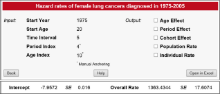
Screen shot of the output page. Additional graphs and tables are displayed when the corresponding check boxes are checked.

Input Data.

To work with the CancerHazard@Age , values of the following variables have to be input: Title, Start Age, Start Year, and Time Interval. In addition, when the manual anchoring is used, two other variables, Periodindex and Age Index, have to be input. Note, when automatic anchoring is used, the tool calculates the Period Index and the Age Index automatically; thus, input of these two variables is not needed. Finally, two matrixes, the Cases and the Populations, saved as a comma-separated-value or a tab-separated-value file, have to be uploaded. The meaning of the input data is explained below.

Title describes the computing work to be executed (for instance, hazard rates of female lung cancers diagnosed in 1975–2005).

Start Age represents the youngest age (in years) of the first age interval (for instance, 20 for the first age interval, 20–24).

Start Year represents the first year of the first time period (for instance, 1975 for the first time period, 1975–1979).

Time Interval represents the width (A) (in years) of the time-period intervals (for instance, 5). Note, the width of the time-period intervals and the width of the age intervals must be equal.

Period Index represents the index (j₀) of the anchored time period. This index can be a number taken from the set of integer numbers, {3, …, m}, where m is the number of the considered time periods. Note, when the automatic anchoring is used, this variable is calculated automatically.

Age Index represents the index (i₀) of the anchored age interval. This index can be a number taken from the set of integer numbers, {1, …, n}, where n is the number of the considered age intervals. Note, this variable is calculated automatically when the automatic anchoring is used.

Cases represents the n × m matrix (O_i,j) with the numbers of the cancers of a specific site/type diagnosed in n successive age intervals (rows) and in m successive time periods (columns). For instance, this matrix can be obtained by copping the raw data from Table 1, while excluding the age index and the age interval columns, as well as all the headers.

Table 1.

Distribution of the female lung cancers (O_i,j) diagnosed in seven time periods.

AGE		NUMBER OF CANCERS IN THE TIME PERIODS (J = 1, …, 7)
INDEX	INTERVAL	1975–79	1980–84	1985–89	1990–94	1995–99	2000–04	2005–09
1	20–24	9	9	14	13	18	11	14
2	25–29	28	23	28	28	19	22	26
3	30–34	64	55	65	84	64	64	74
4	35–39	165	183	181	197	244	167	135
5	40–44	421	450	450	469	467	571	396
6	45–49	839	808	886	969	1004	1099	1179
7	50–54	1348	1568	1475	1594	1659	1730	1919
8	55–59	1839	2285	2426	2349	2382	2659	2551
9	60–64	1995	2760	3342	3286	3145	3250	3535
10	65–69	1735	2858	3607	4320	4307	3755	4030
11	70–74	1320	2208	3239	4054	4594	4373	4189
12	75–79	796	1380	2264	3074	3715	4054	4120
13	80–84	393	689	1087	1560	2147	2580	3106
14	85–89	163	266	403	543	792	1008	1382
15	90–94	28	74	108	135	172	224	322
16	95–99	7	16	26	17	19	35	45

Populations presents the n × m matrix (PoP _i,j ) with the corresponding populations from which the cancer cases were diagnosed. For instance, this matrix can be obtained by copping the raw data from Table 2, while excluding the age index and the age interval columns, as well as all the headers.

Table 2.

Distribution of the female populations (Pop _i,j ) in seven time periods.

AGE		POPULATIONS IN THE TIME PERIOD INTERVALS (J = 1, …, 7)
INDEX	INTERVAL	1975–79	1980–84	1985–89	1990–94	1995–99	2000–04	2005–09
1	20–24	4818118	5022802	4633214	4337370	4200331	4589554	4704432
2	25–29	4576150	5099197	5270726	4983957	4839239	4632896	4934900
3	30–34	3921551	4719961	5219021	5504044	5294338	5050167	4759552
4	35–39	3090013	3819857	4653743	5269860	5596083	5262558	5063586
5	40–44	2734976	3067061	3871091	4758729	5291060	5514007	5228291
6	45–49	2802539	2667562	3017532	3773293	4657456	5181428	5434556
7	50–54	2937860	2740573	2608849	2964492	3777547	4614727	5098668
8	55–59	2714232	2794993	2603976	2518057	2861670	3612048	4483859
9	60–64	2304858	2521021	2591301	2475818	2401406	2690294	3444829
10	65–69	1951631	2177955	2371890	2434845	2307710	2228174	2540365
11	70–74	1550264	1748745	1935514	2114640	2183559	2091997	2053318
12	75–79	1172607	1333155	1509433	1689485	1870856	1930891	1837533
13	80–84	823674	898818	1023052	1174386	1336730	1486723	1566215
14	85–89	393639	497110	576938	674730	792002	886959	1009229
15	90–94	177610	224296	260315	304438	357351	401343	454218
16	95–99	52358	66121	76739	89746	105344	115935	136277

Output Data.

The CancerHazard@Age outputs the following data: (i) Intercept, (ii) Overall Rate, (iii) Age Effects, (iv) Period Effects, (v) Cohort Effects, (vi) Population Rates, and (vii) Individual Rates. The results of the calculation can be presented in graphical and tabular forms by checking the corresponding checkboxes. The numbers shown on a screen are rounded to four digits after the decimal point. Values, smaller than 0.0001, are shown as <0.0001. Results can be opened in Microsoft Excel by clicking the Open in Excel Button. In Excel, the numbers are shown without rounding. The meaning of the output data is explained below.

Intercept shows a constant μ (and its standard error) estimated by solving the system (1).

Overall Rate shows the estimate of the overall population hazard rate, $H_{\text{UO}}^{*}$ (and its standard error).

Age Effects show the estimates of the age effects (and their standard errors). The age effects are presented as graphs (age effects vs. age at diagnosis) and as the corresponding tables.

Period Effects show the estimates of the time-period effects (and their standard errors). The time-period effects are presented as graphs (period effects vs. year of diagnosis) and as the corresponding tables.

Cohort Effects show the estimates of the birth cohort effects (and their standard errors). The birth cohort effects are presented as graphs (cohort effects vs. birth date at diagnosis) and as the corresponding tables. Note, the birth date at diagnosis is referred to by the mid-year of the birth of the cohort.

Population Rates show the estimates of the population cancer hazard rates (and their standard errors). The population rates are presented as graphs (population rates vs. age at diagnosis) and as the corresponding tables.

Individual Rates show the estimates of the individual cancer hazard rates (and their standard errors). The individual rates are presented as graphs (individual rates vs. age at diagnosis) and as the corresponding tables.

Utility of the CancerHazard@Age.

To demonstrate the utility of the CancerHazard@Age , we used data on the female lung cancers diagnosed in 1975–2009 in nine geographic areas within the USA. In the computing experiment performed, the manual anchoring and the following values of the variables (shown in parentheses and in italics) were used: Start Age (20), Start Year (1975), Period Index (4), Age Index (10), and Time Interval (5). Two additional matrixes (Cases and Populations) were uploaded. These matrices (with the numbers of cancer cases and sizes of population, which were determined as described in Materials and Methods) are shown in Tables 1 and 2, correspondingly.

Using these input data and the uploaded files, the CancerHazard@Age determined a unique solution for the system (1). This solution is presented by values of the following variables and the corresponding standard errors (SE): (i) the constant μ (the intercept); (ii) age (A) effects; (iii) period (P) effects; (iv) cohort (C) effects; (v) overall rate; (vi) population rates; and (vii) individual rates. Specifically, the estimated value of the intercept was −7.9572 with the SE of 0.0159. The obtained estimates of the A, P, and C effects (and their SE) are shown in Tables 3–5, correspondingly. The estimated value (given in units of the number of cancer cases per 100,000 person-years) of the overall rate was 1363.434 with the SE of 17.607. The obtained estimates of the population and individual rates (and their SE) are shown in Tables 6 and 7, correspondingly.

Table 3.

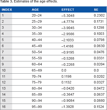
Estimates of the age effects.

INDEX	AGE	EFFECT	SE
1	20–24	−5.3048	0.2302
2	25–29	−4.7774	0.1731
3	30–34	−3.9045	0.1298
4	35–39	−2.9566	0.1003
5	40–44	−2.1033	0.0798
6	45–49	−1.4166	0.0630
7	50–54	−0.9195	0.0476
8	55–59	−0.5268	0.0331
9	60–64	−0.2268	0.0204
10	65–69	0.0	0.0
11	70–74	0.1198	0.0202
12	75–79	0.1132	0.0327
13	80–84	−0.0420	0.0472
14	85–89	−0.3647	0.0637
15	90–94	−0.9084	0.0880
16	95–99	−1.3928	0.1524

Table 4.

Estimates of the period effects.

INDEX	PERIOD	EFFECT	SE
1	1975–79	−0.4038	0.0406
2	1980–84	−0.2044	0.0266
3	1985–89	−0.0770	0.0
4	1990–94	0.0	0.0
5	1995–99	0.0507	0.0246
6	2000–04	0.0850	0.0382
7	2005–09	0.1528	0.0524

Table 5.

Estimates of the cohort effects.

INDEX	COHORT	EFFECT	SE
1	1880	−0.7756	0.5975
2	1885	−0.8357	0.2620
3	1890	−0.5907	0.1407
4	1895	−0.7178	0.1038
5	1900	−0.5850	0.0807
6	1905	−0.4195	0.0629
7	1910	−0.2370	0.0473
8	1915	−0.0891	0.0332
9	1920	−0.0405	0.0207
10	1925	0.0	0.0
11	1930	−0.0150	0.0207
12	1935	−0.1137	0.0333
13	1940	−0.2483	0.0472
14	1945	−0.4662	0.0617
15	1950	−0.7366	0.0771
16	1955	−0.8050	0.0930
17	1960	−0.8204	0.1102
18	1965	−1.1568	0.1346
19	1970	−1.2870	0.1712
20	1975	−0.9857	0.2164
21	1980	−1.2386	0.3166
22	1985	−1.2252	0.4783

Table 6.

Estimates of the population rates.

INDEX	AGE	RATE	SE
1	20–24	0.1739	0.0401
2	25–29	0.2947	0.0512
3	30–34	0.7056	0.0923
4	35–39	1.8206	0.1848
5	40–44	4.2734	0.3479
6	45–49	8.4922	0.5522
7	50–54	13.9604	0.7017
8	55–59	20.6740	0.7604
9	60–64	27.9058	0.7225
10	65–69	35.0128	0.5599
11	70–74	39.4679	1.0154
12	75–79	39.2109	1.4290
13	80–84	33.5718	1.6742
14	85–89	24.3108	1.5976
15	90–94	14.1160	1.2623
16	95–99	8.6961	1.3322

Table 7.

Estimates of the individual rates.

INDEX	AGE	RATE	SE
1	20–24	0.0001	<0.0001
2	25–29	0.0002	<0.0001
3	30–34	0.0005	<0.0001
4	35–39	0.0013	0.0001
5	40–44	0.0032	0.0003
6	45–49	0.0065	0.0004
7	50–54	0.0112	0.0006
8	55–59	0.0178	0.0007
9	60–64	0.0268	0.0008
10	65–69	0.0396	0.0010
11	70–74	0.0565	0.0020
12	75–79	0.0782	0.0037
13	80–84	0.1051	0.0067
14	85–89	0.1390	0.0121
15	90–94	0.1792	0.0232
16	95–99	0.4000	0.0867

For the female lung cancers, Figure 3 shows how the age (A) effects depend on the age at diagnosis. The values of these effects and their SE are presented in Table 3. Figure 3 and Table 3 show that up to the age of 70, the age effects increase with the increase in the age at diagnosis, reach the maximum at the age interval of 70–74, and fall at older ages.

Figure 3.

Female lung cancer occurrence: age effects vs. age at diagnosis. Filled circles present the age (A) effects for mid-points (mid-age) of the age intervals at which the cancer diagnosis was performed. Bars show the 95% confidence intervals (CIs) of the A effects. The solid line shows the trend of the A effects. The triangle presents the anchored A effect.

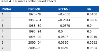
Figure 4 shows how the period (P) effects depend on the period of diagnosis. The values of these effects and their SE are presented in Table 4. As can be seen from Figure 4 and Table 4, the trend of the P effects continuously increases when the period (date) of the cancer diagnosis increases.

Figure 4.

Female lung cancer occurrence: time-period effects vs. time period of diagnosis. Filled circles present the time-period (P) effects for the mid-points (mid-dates, in years) of the corresponding time-period intervals within which the cancer diagnosis was performed. Bars show the 95% CI of the P effects. The solid line shows the trend of the P effects. The triangle presents the anchored P effect. The diamond presents the identification parameter.

Figure 5 shows the birth cohort (C) effects vs. the year of the cohort birth. The values of these effects and their SE are presented in Table 5. A mid-year birth of the cohort considered at the date of diagnosis is considered as the year of the cohort birth. Figure 5 and Table 5 show that the trend of the C effects, referred to by 1880, 1985, …, and 1920, increases with an increase in the mid-year of the cohort birth; reaches a maximum for the cohort referred to by 1925; falls for the cohorts referred to by 1930, 1935, …, 1960; and almost flattens for the cohorts referred to by 1965, 1970, …, 1985.

Figure 5.

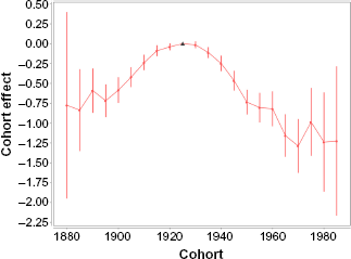
Female lung cancer occurrence: birth cohort effects vs. year of the cohort birth. Filled circles present the birth cohort (C) effects for the mid-year of the cohort birth. Bars show the 95% CI of the C effects. The solid line shows the trend of the C effects. The triangle shows the anchored C effect.

Figure 6 shows the population rates vs. age at diagnosis. The estimates of these rates and their SE are presented in Table 6. These estimates are given in units of the number of cancer cases per 100,000 person-years. Figure 6 and Table 6 suggest that the trend of the population rates increases up to the age of 70, reaches a maximum at the 70–74 age interval, and falls at older ages.

Figure 6.

Female lung cancer occurrence: population hazard rates vs. age at diagnosis. Filled circles present the population hazard rates for the mid-points of the age intervals at which the cancer diagnosis was performed. Bars show the 95% CI of the population hazard rates. The rates and their CI are given in units of the number of cancer cases per 100,000 person-years. The solid line shows the trend of the population hazard rates. The triangle presents the anchored population hazard rate.

Figure 7 shows the individual rates vs. age at diagnosis. The estimates of these rates and their standard errors are presented in Table 7. These estimates are given in units of the number of cancer cases per 100,000 person-years. (It should be noted that the point presenting the individual rates in the 95–99 age interval is not shown in Figure 7. The individual rates are inaccurately estimated in that age interval because of the fact that a very small number of women susceptible to lung cancer are alive at the ages of 95 and older.) Figure 7 and Table 7 suggest that the trend of the individual rates increases, with an increase in the age at diagnosis.

Figure 7.

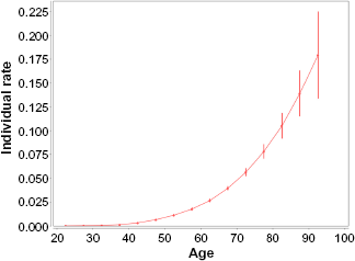
Female lung cancer occurrence: individual hazard rates vs. age at diagnosis. Filled circles present the individual hazard rates for mid-points of the age intervals at which the cancer diagnosis was performed. Bars show the 95% CI of the individual hazard rates. The rates and their CI are given in units of the number of cancer cases per 100,000 person-years. The solid line shows the trend of the individual hazard rates.

Main Distinguishable Features of the CancerHazard@Age.

Conceptually, the CancerHazard@Age tool presented in this work is closely related to the AgePeriodCohort tool that was recently published in Ref. 10. Both tools use the past and current history of cancer incidences collected during a long time period in the surveillance databases to perform the APC analysis. These tools also share the main limitations of the descriptive analysis; however, the CancerHazard@Age tool and the AgePeriodCohort tool use different mathematical approaches and different assumptions. The ability of further use of the results obtained by these tools depends on the competency of the assumptions used for solving the identifiably problem. Specifically, the goodness of estimable parameters and functions determined by the AgePeriodCohort tool depends on the competency of several null hypotheses (see Table 2 in Ref. 10). Analogously, the goodness of a solution provided by the CancerHazard@Age tool depends on the fact that the effects of the adjacent cohorts on cancer hazard in aging are close. ⁷ Such an assumption, however, appears to be a mild constrain in comparison with constrains (null hypotheses) used in Ref. 10. For a given set of input data, the validity of using the LLAPC model for the APC analysis by the CancerHazard@Age tool can be checked by using several plots ⁷ : (i) the normal probability plot of the standardized residuals, (ii) the residuals vs. the modeled values plot, and (iii) the observed vs. the modeled values plot.

The CancerHazard@Age tool uses the estimated APC effects for calculating the overall cancer hazard rate, as well as the population and individual cancer hazard rates. The concept of the overall hazard rate extends the concept of the age-adjusted incidence rate, commonly used in cancer epidemiology. A distinguished feature of the overall rate is in accounting for the APC effects. Analogously, the concept of the population cancer hazard rates extends the concepts of the cross-sectional (period-specific) and longitudinal (cohort-specific) age-specific incidence rates. The CancerHazard@Age also implements the novel concept of the individual hazard rates recently introduced in Ref. 6.

The population and individual cancer hazard rates can be further analyzed by methods of statistical modeling (such as proportional hazards, confounding factors, interaction, and effect modification). The overall cancer hazard rate and the population and individual cancer hazard rates determined by the CancerHazard@Age can be used for purposes of descriptive and interferential statistics. Mathematical modeling of the population and individual hazard rates can shed light on the intrinsic propensity of cancer development in distinct organ sites. Analysis of the temporal trends of the APC effects, determined by this tool, can be used for projecting future cancer burden.

Author Contributions

Conceived and designed the experiments: TM, AS, OS, SS. Analyzed the data: TM, AS, OS, SS. Wrote the first draft of the manuscript: TM, SS. Contributed to the writing of the manuscript: TM, AS, OS, SS. Agree with manuscript results and conclusions: TM, AS, OS, SS. Jointly developed the structure and arguments for the paper: TM, AS, OS, SS. Made critical revisions and approved final version: SS. All authors reviewed and approved of the final manuscript.