Basic Equations and Computing Procedures for Frailty Modeling of Carcinogenesis: Application to Pancreatic Cancer Data

Abstract

Modeling of cancer hazards at age t deals with a dichotomous population, a small part of which (the fraction at risk) will get cancer, while the other part will not. Therefore, we conditioned the hazard function, h(t), the probability density function (pdf), f(t), and the survival function, S(t), on frailty α in individuals. Assuming α has the Bernoulli distribution, we obtained equations relating the unconditional (population level) hazard function, h_U(t), cumulative hazard function, H_U(t), and overall cumulative hazard, H₀, with the h(t), f(t), and S(t) for individuals from the fraction at risk. Computing procedures for estimating h(t), f(t), and S(t) were developed and used to ft the pancreatic cancer data collected by SEER9 registries from 1975 through 2004 with the Weibull pdf suggested by the Armitage-Doll model. The parameters of the obtained excellent fit suggest that age of pancreatic cancer presentation has a time shift about 17 years and five mutations are needed for pancreatic cells to become malignant.

Introduction

Mathematical modeling of cancer hazards in aging is aimed at determining the relationship between the observed cancer incidences in the population with the carcinogenic processes ongoing in individuals. At the present time, many different carcinogenetic models have been developed in which the hazard of getting cancer in aging is considered as a random process. The main difference between these models is in accounting the variability of the hazard of getting cancer within individuals. Some of the models assume that all individuals initially have equal chances of getting cancer,^1,2 while other models assume that within individuals these chances are randomly distributed and introduce a nonnegative random variable (a frailty) that is multiplied with the hazard to cancer. ³

Modeling of cancer hazards in aging requires the use of a theoretical hazard function and, when frailty is assumed, a frailty distribution function. As hazard functions, linear functions, ¹ exponential functions, ⁴ beta-functions,^5,6 and some other functions have been used. ⁷ As frailty, the gamma-distribution, compound Poisson distribution, power-variance distribution, as well as other distributions, have been utilized.^8–12 Mathematically, the problem of modeling is stated as a best fitting of the hazard rates with observations using methods of regression analysis. The obtained models are useful when the utilized model parameters have apparent biological meaning and the estimated values of these parameters are consistent with the estimates presented by biological means. Unfortunately, often these models are very complicated and do not agree with the observed data. In addition, some model parameters do not have clear biological meaning, and/or their values are inconsistent with the estimates provided by the current knowledge on the carcinogenetic processes ongoing in individuals. ³

In the present work, for a better accounting for cancer hazards on individual and population levels, we utilized the main concepts of survival analysis (the survival function, S(t), the hazard function, h(t), and the probability density function (pdf), f(t)), and conditioned these functions on frailty α used on an individual level. We assumed that the population under consideration is a dichotomous one: a small part of this population (so called fraction at risk) will eventually get the cancer, ⁹ while the other part (immune fraction) will not. In such a case, it is appropriate to present the frailty α by the Bernoulli distribution. Based on the main concepts of survival analysis and the mathematical statistics,^13,14 we developed novel equations and a computing framework to be used in carcinogenetic modeling. We suggested that these equations and the computing framework can be applied to estimate the parameters of different carcinogenic models with a given f(t) (or h(t), or S(t)) on the individual levels. As an example, we used the Weibull pdf, suggested by the Armitage-Doll multiple mutation model of carcinogenesis, and estimated the model parameters of the pancreatic cancer occurrence in aging using the corresponding data collected by SEER9 registries from 1975 through 2004.

Basic Equations for Frailty Modeling of Cancer Hazards in Aging

To determine the relationship between the estimates of the hazard function performed for the dichotomous population (population level) with the survival, hazard, and probability density functions determined on the individual level, we utilized the concept of frailty. We presented variability to cancer susceptibility between individuals in the dichotomous population using the Bernoulli distribution, which provides a binary presentation (1/0) to the statistical distribution of individuals within the considered population, assuming that “1” means that an individual belongs to the fraction at risk and eventually will get cancer, while “0” means that this individual belongs to the immune fraction and will not get cancer.

Main Concepts for Modeling of Cancer Hazards in Aging for Individuals from the Fraction at Risk

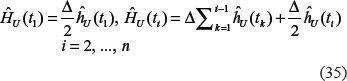
The concepts of survival function, S(t), a hazard function, h(t) and a probability density function (pdf), f(t), developed in “classical” survival analysis can be directly used for the mathematical presentation of events occurring in the fraction at risk. In this case, the event time, t, refers to the age of an individual when a cancer is diagnosed and the survival function, S(t), can be defined as:

$$S\left(t\right)=1-F\left(t\right)$$

(1)

where F(t) is a cumulative frequency function (or a cumulative distribution function, cdf), which refers to the probability that in an individual, a considered event will occur up to the time t. This function can be presented as:

$$F\left(t\right)={\displaystyle {\int }_0^{t}f\left(u\right)du}$$

(2)

By definition, a hazard function, h(t), is determined by formula ¹³ :

$$h\left(t\right)=\frac{-d\left[S\left(t\right)\right]/dt}{S\left(t\right)}$$

(3)

From (1)–(3) it follows:

$$h\left(t\right)=\frac{f\left(t\right)}{S\left(t\right)}$$

(4)

Note that by specifying the probability density function, f(t), or the survival function, S(t), or the hazard function, h(t), the other two functions can be ascertained. For example, if f(t) is the Weibull pdf, then the corresponding hazard function, h(t), will be an exponential function of tand ln[-ln S(t)] is a linear function with ln t.

Basic Equations for Modeling of Cancer Hazards in Aging for Individuals from the Dichotomous Population

In frailty models, the basic hazard rate, h(t), is multiplied with the frailty positive random variable α. The frailty random variable expresses the extent of frailty in each individual. A large value of αreflects that an individual is highly susceptible to cancer, whereas a low value characterizes an individual that is less susceptible to cancer. The individual hazard rate and survival function conditioned on frailty can be expressed as ¹³ :

$$h\left(t|\alpha \right)=\alpha h\left(t\right)$$

(5)

and

$$S\left(t|\alpha \right)=S{\left(t\right)}^{\alpha }$$

(6)

When the frailty distribution with the pdf, g(α), is known from the conditional survival function, S(t|α), which is determined on the individual level, one can obtain unconditional survival function, S_U(t), and the unconditional hazard function, h_U(t), on the population level. In fact, for the population under consideration, we have: ¹³

$$S_U\left(t\right)={\displaystyle {\int }_0^{\infty }S\left(t|\alpha \right)g\left(\alpha \right)d\alpha }$$

(7)

Note that if αis a discreet random variable, α= α_N, N= 1,2…, with probability distribution g(α_N) = g_N, then instead of (7) we have:

$$S_U\left(t\right)={\displaystyle \sum _{N}S\left(t|{\alpha }_N\right)g_N}$$

(8)

and by definition: ¹³

$$h_U\left(t\right)=\frac{-d\left[S_U\left(t\right)/dt\right]}{S_U\left(t\right)}$$

(9)

Based on the fact that only a small part of the population (fraction at risk) is exposed to the cancer, while the other part of the population (immune fraction) is not, we assumed that the frailty αcan also take the value of zero (that means that the individual is immune to the cancer) and that the frailty αhas the Bernoulli distribution with the parameter, p, which is a probability that a given individual will eventually get the cancer. The Bernoulli distribution, which in mathematical statistics is usually designated as B(1,p), has the following discreet pdf:

$$g\left(\alpha =0\right)=1-p$$

(10)

and

$$g\left(\alpha =1\right)=p$$

(11)

In such a case, according to (6) and (8), we have:

$$S_U\left(t\right)=S^0\left(t\right)\cdot \left(1-p\right)+S^1\left(t\right)\cdot p=1-p+pS\left(t\right)$$

(12)

Taking into account (1), (2), (9), and (12) we have:

$$h_U\left(t\right)=\frac{pf\left(t\right)}{1-p{\displaystyle {\int }_0^{t}f\left(u\right)du}}$$

(13)

For the majority of cancer types, p < 1 (because a particular type of cancer is a rare disease) and the denominator of the right side of the (13) is very close to 1. Therefore, from formula (13) it follows that h_U(t) can be approximated by pf(t):

$$h_U\left(t\right)=pf\left(t\right)$$

(14)

(Below, without losing generosity, we considered formula (14) as a precise equality).

According to (14), in the age-specific population, the age-specific hazard function is proportional to pdf, f(t), of ages at which individuals from the fraction at risk will get cancer. Taking into account that ${\displaystyle {\int }_0^{\infty }f\left(t\right)dt=1}$ , the parameter, p, can be easily obtained by integrating both sides of (14):

$$p={\displaystyle {\int }_0^{\infty }{h}_U\left(t\right)dt}$$

(15)

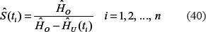
On the other hand, by definition, the overall cumulative unconditional hazard rate, H₀, is determined as:

$$H_0=H_U\left(\infty \right)={\displaystyle {\int }_0^{\infty }{h}_U\left(t\right)dt}$$

(16)

where

$$H_U\left(t\right)={\displaystyle {\int }_0^t{h}_U\left(\tau \right)d\tau }$$

(17)

is the unconditional cumulative hazard rate. Thus, from (15) and (16) it follows that, on the population level, the overall cumulative unconditional hazard, H₀, characterizes the fraction at risk in the dichotomous population and is equal to p.

Finally, by dividing both sides of (14) on pand substituting pon H₀we can obtain that:

$$\frac{h_U\left(t\right)}{H_o}=f\left(t\right)$$

(18)

The equation (18) relates the hazard function, h_U(t), and the overall hazard, H_O, on the population level with the pdf, f(t), on the individual level. The left side of (18) can be estimated from the observed data. We consider (18) as a basic equation for estimating the unknown model parameters of f(t) based on values of h_U(t) and H_Othat can be estimated from the observed data. As we show below, the problem of estimating the model parameters of f(t) from the values of h_U(t) and H_Ois reduced to the problem of solving the corresponding system of the conditional equations.

Using (1) to (4) and (18), after elementary transformations, one can obtain the following two equations:

$$\frac{h_U\left(t\right)}{H_o-H_U\left(t\right)}=h\left(t\right)$$

(19)

and

$$\frac{H_o}{H_o-H_U\left(t\right)}=S\left(t\right)$$

(20)

These equations can also be used for forming the system of the conditional equations from which unknown parameters of model hazard and survival functions can be estimated.

Computing Procedures for Modeling of Cancer Hazards in Aging

Below we propose computing procedures for modeling cancer hazards in aging by using the observed data on the population level (presented in a discrete tabulated form) and a theoretical form of the pdf, f(t), given on the individual level. In a discrete form, to solve the problem of modeling of cancer hazards in aging, the following three procedures need to be consecutively executed.

Procedure 1: Estimation of the Age-Specific Hazard Rates by the Age-Period-Cohort(Apc)Analysis

Let us assume that the observed numbers of cancer cases and the numbers of population in the equal-sized consecutive nage intervals, ${{\Delta }^{\prime }}_i\left(\left|{{\Delta }^{\prime }}_i\right|=\Delta ;i=1,2,\dots ,n\right)$ , and mconsecutive time-period intervals, ${{\Delta }^{″}}_i\left(\left|{{\Delta }^{″}}_i{}_i\right|=\Delta ;j=1,2,\dots ,m\right)$ , are known. In cancer registries, the cancer incidences and the size of population are usually tabulated with five-year age intervals and five-year timeperiod intervals (ie, δ = 5). Such tables have nrows, associated with the age intervals, and mcolumns, associated with the time-period intervals. The estimates of the age-specific incidence crude rates for each i,j cell of a cancer registry table, ${\widehat{I}}_{i,j}\left(t_i\right)$ , and their standard errors, $S\widehat{E}\left[{\widehat{I}}_{i,j}\left(t_i\right)\right]$ , can be determined as: ¹⁵

$${\widehat{I}}_{i,j}\left(t_i\right)=\frac{m_{i,j}}{\Delta P_{i,j}},\hspace{1em}i=1,2,\dots ,n$$

(21)

and

$$S\widehat{E}\left[{\widehat{I}}_{i,j}\left(t_i\right)\right]=\frac{\sqrt{m_{i,j}}}{\Delta P_{i,j}},\hspace{1em}i=1,2,\dots ,n$$

(22)

where t_iis the midpoint of the i-th age interval (i= 1,2, …, n). (Here and below symbols “^” designate the corresponding estimates.) In (21) and (22), m_i,jand P_i,jare the number of cancer cases and the size of population in the i-th age interval, observed during the j-th time-period, correspondingly.

According to the log-linear age-period-cohort (LLAPC) model, the observed age-specific incidence rates can be presented as:^16–18

$${\widehat{I}}_{i,j}\left(t_i\right)=v_j{u}_l{h}_U\left(t_i\right),\hspace{1em}i=1,2,\dots ,n,\hspace{1em}j=1,2,\dots ,m$$

(23)

where v_jand u_iare the time-period and birth-cohort effects, correspondingly, and h_U(t_i) are the values of the unknown hazard function at age, t_i, to be estimated from the system of the conditional equations (23). In (23), the index lis defined by a linear combination of the age and time-period indexes in the following way:

$$l=j-i+n\hspace{1em}\left(l=1,2,\dots ,k\right)$$

(24)

From system (23) it follows that, when the time-period and birth-cohort effects are negligible (v_j ≅ 1 and u_l ≅ 1), the best estimates of the hazard function values, ${\widehat{h}}_U\left(t_i\right)$ , will be the weighted means of the incidence rates:

$${\widehat{h}}_U\left(t_i\right)=\frac{{\displaystyle {\sum }_{j=1}^m{W}_{i,j}{\widehat{I}}_{i,j}\left(t_i\right)}}{{\displaystyle {\sum }_{j=1}^m{W}_{i,j}}}\hspace{1em}i=1,2,\dots ,n\hspace{1em}j=1,2,\dots ,m$$

(25)

where weights, W_i,j, can be calculated using formula (22) as:

$$W_{i,j}=\frac{1}{S{\widehat{E}}^2\left[{\widehat{I}}_{i,j}\left(t_i\right)\right]}\hspace{1em}i=1,2,\dots ,n$$

(26)

and

$$S{\widehat{E}}^2\left[{\widehat{h}}_U\left(t_i\right)\right]=\frac{1}{{\displaystyle {\sum }_{j=1}^{m}1/S{\widehat{E}}^2\left[{\widehat{I}}_{i,j}\left(t_i\right)\right]}}\hspace{1em}i=1,2,\dots ,n$$

(27)

When the time-period and birth-cohort effects are significant, the estimates, ${\widehat{h}}_u\left(t_i\right)$ , can be obtained by the age-period-cohort (APC) analysis. Recently, ¹⁹ we proposed an efficient computational procedure for determining the APC effects in the frame of the LLAPC model and demonstrated how this procedure can be used in practice.

Procedure 2: Estimation of the Pdf, Cdf, Hazard, and Survival Functions on the Individual Level

To estimate f(t), we will use the equation (18) that presents a relationship between the values of the hazards of getting cancer in aging and f(t). In a discrete form, the estimates $\widehat{f}\left(t_i\right)$ can be obtained from formula (18) by substituting h_U(t) and H_Owith their estimates:

$$\widehat{f}\left(t_i\right)=\frac{{\widehat{h}}_U\left(t_i\right)}{{\widehat{H}}_o}\hspace{1em}i=1,2,\dots ,n$$

(28)

In (28), ${\widehat{h}}_U\left(t_i\right)$ , are determined by formula (25), and according to (16), ${\widehat{H}}_o$ can be determined as:

$${\widehat{H}}_o={\displaystyle {\sum }_{i=1}^n{\widehat{h}}_U\left(t_i\right)\Delta \hspace{1em}i=1,2,\dots ,n}$$

(29)

Standard errors of $\widehat{f}\left(t_i\right)$ can be obtained by the simulation experiments in the following way ¹⁴ Assuming that the errors follow a Gaussian distribution around ${\widehat{h}}_U\left(t_i\right)$ with known $S\widehat{E}\left[{\widehat{h}}_U\left(t_i\right)\right]$ , one can simulate, via equations (28) and (29), the estimated values of $\widehat{f}\left(t_i\right)$ for many times and then obtain the estimates, $S\widehat{E}\left[\widehat{f}\left(t_i\right)\right]$ , in a standard way. An alternative way for obtaining $S\widehat{E}\left[\widehat{f}\left(t_i\right)\right]$ is to use the standard rules of error propagation. ²⁰ Our computational experiments showed that these two approaches give nearly the same results. Below, $S\widehat{E}\left[\widehat{f}\left(t_i\right)\right]$ is obtained by the standard rules of error propagation. ²⁰

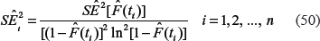
Assuming that a correlation between errors of the ${\widehat{H}}_o$ and ${\widehat{h}}_U\left(t_i\right)$ is negligible, and using standard rules of error propagation, we presented the standard errors of ${\widehat{H}}_o$ and $\widehat{f}\left(t_i\right)$ as:

$$S{\widehat{E}}^2\left[{\widehat{H}}_o\right]={\Delta }^2{\displaystyle {\sum }_{i=1}^{n}S{\widehat{E}}^2\left[{\widehat{h}}_U\left(t_i\right)\right]\hspace{1em}i=1,2,\dots ,n}$$

(30)

$$S{\widehat{E}}^2\left[\widehat{f}\left(t_i\right)={\left(\frac{{\widehat{h}}_U\left(t_i\right)}{{\widehat{H}}_o}\right)}^2\left\{\frac{S{\widehat{E}}^2\left[{\widehat{h}}_U\left(t_i\right)\right]}{{\left[{\widehat{h}}_U\left(t_i\right)\right]}^2}+\frac{S{\widehat{E}}^2\left({\widehat{H}}_o\right)}{{\widehat{H}}_o{}^2}\right\}\right]\hspace{1em}i=1,2,\dots ,n$$

(31)

Estimates of the cumulative distribution function (cdf) $\widehat{F}\left(t_i\right)$ , and the estimates of their standard errors, $S\widehat{E}\left[\widehat{F}\left(t_i\right)\right]$ , can be obtained as follows:

$$\widehat{F}\left(t_1\right)=\frac{\Delta }{2}\widehat{f}\left(t_1\right),\widehat{F}\left(t_i\right)=\Delta {\displaystyle {\sum }_{k=1}^{i=1}\widehat{f}\left(t_k\right)+\frac{\Delta }{2}\widehat{f}\left(t_i\right)\hspace{1em}i=2,\dots ,n}$$

(32)

$$\begin{array}{c}S{\widehat{E}}^2\left[\widehat{F}\left(t_i\right)\right]=\frac{{\Delta }^2}{4}S{\widehat{E}}^2\left[\widehat{f}\left(t_1\right)\right],S{\widehat{E}}^2\left[\widehat{F}\left(t_i\right)\right]\\ ={\Delta }^2{\displaystyle {\sum }_{k=1}^{i=1}S{\widehat{E}}^2\left[\widehat{f}\left(t_i\right)\right]+\frac{{\Delta }^2}{4}S{\widehat{E}}^2\left[\widehat{f}\left(t_i\right)\right],\hspace{1em}i=2,\dots n}\end{array}$$

(33)

where t_k is the midpoint of the interval, Δ_k, and $\widehat{f}\left(t_i\right)$ and $S\widehat{E}\left[\widehat{f}\left(t_i\right)\right]$ are given by formulas (28) and (31), correspondingly.

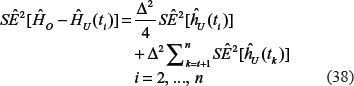
Analogously, to estimate the hazard and survival functions on the individual level from the observed data in a discrete form, the systems of conditional equations can be constructed on the basis of the equations (19) and (20). For estimates of the hazard function on the individual level we obtained:

$$\widehat{h}\left(t_i\right)=\frac{{\widehat{h}}_U\left(t_i\right)}{{\widehat{H}}_o-{\widehat{H}}_U\left(t_i\right)}\hspace{1em}i=1,2,\dots ,n$$

(34)

where ${\widehat{H}}_o$ is the estimate of the overall hazard given by formula (28). The estimate of the cumulative hazard, ${\widehat{H}}_U$ , is obtained as:

$${\widehat{H}}_U\left(t_1\right)=\frac{\Delta }{2}{\widehat{h}}_U\left(t_1\right),{\widehat{H}}_U\left(t_i\right)=\Delta {\displaystyle {\sum }_{k=1}^{i-1}{\widehat{h}}_U\left(t_k\right)+\frac{\Delta }{2}{\widehat{h}}_U\left(t_i\right)\hspace{1em}i=2,\dots ,n}$$

(35)

$$\begin{array}{c}S{\widehat{E}}^2\left[{\widehat{H}}_U\left(t_1\right)\right]=\frac{{\Delta }^2}{4}S{\widehat{E}}^2\left[{\widehat{h}}_U\left(t_1\right)\right],S{\widehat{E}}^2\left[{\widehat{H}}_U\left(t_i\right)\right]\\ ={\Delta }^2{\displaystyle {\sum }_{k=1}^{i-1}S{\widehat{E}}^2\left[{\widehat{h}}_U\left(t_k\right)\right]+\frac{{\Delta }^2}{4}S{\widehat{E}}^2\left[{\widehat{h}}_U\left(t_i\right)\right]\hspace{1em}i=2,\dots ,n}\end{array}$$

(36)

It is easy to show that

$${\widehat{H}}_o-{\widehat{H}}_U\left(t_i\right)=\frac{\Delta }{2}{\widehat{h}}_U\left(t_i\right)+\Delta {\displaystyle {\sum }_{k=i+1}^n{\widehat{h}}_U\left(t_k\right)\hspace{1em}i=2,\dots ,n}$$

(37)

and

$$S{\widehat{E}}^2\left[{\widehat{H}}_o-{\widehat{H}}_U\left(t_i\right)\right]=\frac{{\Delta }^2}{4}S{\widehat{E}}^2\left[{\widehat{h}}_U\left(t_i\right)\right]+{\Delta }^2{\displaystyle {\sum }_{k=i+1}^{n}S{\widehat{E}}^2\left[{\widehat{h}}_U\left(t_k\right)\right]\hspace{1em}i=2,\dots ,n}$$

(38)

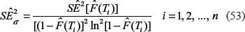
According to (34), using the standard rules of error propagation, we have:

$$S{\widehat{E}}^2\left[\widehat{h}\left(t_i\right)\right]=\frac{{\left[{\widehat{h}}_U\left(t_i\right)\right]}^2}{{\left[{\widehat{H}}_o-{\widehat{H}}_U\left(t_i\right)\right]}^2}\left\{\frac{S{\widehat{E}}^2\left[{\widehat{h}}_U\left(t_i\right)\right]}{{\left[{\widehat{h}}_U\left(t_i\right)\right]}^2}+\frac{S{\widehat{E}}^2\left[{\widehat{H}}_o-{\widehat{H}}_U\left(t_i\right)\right]}{{\left[{\widehat{H}}_o-{\widehat{H}}_U\left(t_i\right)\right]}^2}\right\}\hspace{1em}i=2,\dots ,n$$

(39)

where estimates: $\widehat{h}\left(t_i\right),S{\widehat{E}}^2\left[\widehat{h}\left(t_i\right)\right],{\widehat{h}}_U\left(t_i\right),S{\widehat{E}}^2\left[{\widehat{h}}_U\left(t_i\right)\right],{\widehat{H}}_o-{\widehat{H}}_u$ and $\text{S}{\widehat{E}}^2\left[{\widehat{H}}_o-{\widehat{H}}_u\left(t_i\right)\right]$ are given by formulas (34), (39), (25), (27), (37), and (38), correspondingly.

For estimates of the survival function on the individual level we have:

$$\widehat{S}\left(t_i\right)=\frac{{\widehat{H}}_o}{{\widehat{H}}_o-{\widehat{H}}_U\left(t_i\right)}\hspace{1em}i=1,2,\dots ,n$$

(40)

Note that

$$\widehat{S}\left(t_i\right)=1-\widehat{F}\left(t_i\right)\hspace{1em}i=1,2,\dots ,n$$

(41)

and

$$S{\widehat{E}}^2\left[\widehat{S}\left(t_i\right)\right]=S{\widehat{E}}^2\left[\widehat{F}\left(t_i\right)\right]\hspace{1em}i=1,2,\dots ,n$$

(42)

where $\widehat{F}\left(t_i\right)$ and $S{\widehat{E}}^2\left[\widehat{F}\left(t_i\right)\right]$ are given by formulas (32) and (33), correspondingly.

So, we have shown that $\widehat{f}\left(t_i\right),\widehat{h}\left(t_i\right)$ and $\widehat{S}\left(t_i\right)$ (and their standard errors) on the individual level can be simply obtained from the estimates of the cancer hazard function, ${\widehat{h}}_U\left(t_i\right)$ , (and their standard errors) determined on the population level from the observed data.

Procedure 3: Estimation of the Model Pdf(or Cdf)Parameters

Based on the theoretical models of carcinogenesis, one might assume that the f(t) ought to follow to some nonlinear (in a general case) function f of age, t, defined with the s parameters, ${\tilde{a}}_1,{\tilde{a}}_2,\dots ,{\tilde{a}}_s:f\left({\tilde{a}}_1,{\tilde{a}}_2,\dots ,{\tilde{a}}_s;t\right)$ . In such case, the cdf, F(t), will also be defined by the same sparameters: $F\left({\tilde{a}}_1,{\tilde{a}}_2,\dots ,{\tilde{a}}_s;t\right)$ . To estimate these parameters, one can consider the system of conditional equations:

$$\widehat{f}\left(t_i\right)=f\left({\tilde{a}}_1,{\tilde{a}}_2,\dots ,{\tilde{a}}_s;t_i\right)\hspace{1em}i=1,2,\dots ,n$$

(43)

with the weights, w_i, determined as:

$$w_i=\frac{1}{S{\widehat{E}}^2\left[\widehat{f}\left(t_i\right)\right]}\hspace{1em}i=1,2,\dots ,n$$

(44)

where t_i is the midpoint of the i-th age interval and $\widehat{f}\left(t_i\right)$ is the estimate of the pdf at age t_i, derived from the observations.

Note that we have one response variable, that is the pdf of age, f(t), and one predictor variable, the age t. The predictor is assumed to be measured with no error, while the response data can be affected by an observational error. In general, to obtain the estimates ${\widehat{\tilde{a}}}_1,{\widehat{\tilde{a}}}_2,\dots ,{\widehat{\tilde{a}}}_s$ , the model function, $f\left({\tilde{a}}_1,{\tilde{a}}_2,\dots ,{\tilde{a}}_s;t_i\right)$ with the known observed estimates, $\widehat{f}\left(t_i\right)$ , one can utilize a weighted least squares method. ¹⁴

The aforementioned computational procedure can be applied for determining parameters of different pdf (or cdf) with known mathematical forms. However, for modeling of the cancer occurrence in aging, the mathematical form of the pdf (or cdf) should be chosen by considering the appropriate biological concepts, leading to carcinogenesis. The parameters of this function should have distinct biological and/or epidemiological meaning.

As an example, let us assume that according to the multiple mutation carcinogenic model, the cancer occurrence in aging on the individual level can be represent with a two- or three-parameter Weibull pdf:^4,21,22

$$f\left(\lambda ,r;t\right)=\lambda r^{r-1}\exp \left(-\lambda t^r\right)$$

(45)

and

$$f\left(\lambda ,r;t\right)=\lambda r{\left(t-A\right)}^{r-1}\exp \left[-\lambda {\left(t-A\right)}^r\right]$$

(46)

where the λ is a “scale” parameter, t denotes age, r is a “shape” parameter, and A is a “shift” parameter (according to designations of (43), $\lambda ={\tilde{a}}_1,r={\tilde{a}}_2$ and $A={\tilde{a}}_3$ ). The shift parameter, A, was introduced into the carcinogenesis modeling more than 40 years ago, ⁴ where the effective exposure period, T = t – A, was used to improve the quality of curve fitting for prostate cancer.

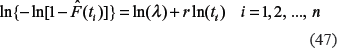
For two-parameter Weibull distribution, when the estimates of the cdf, $\widehat{F}\left(t_i\right)$ , and their standard errors, $S{\widehat{E}}^2\left[\widehat{F}\left(t_i\right)\right]$ in the age intervals, t_i(i = 1,2, …, n), are known from observations, the following linear system of conditional equations with regard to unknown parameters, ln(λ) and r, can be written (note that here the response variable is ln{–ln[1–F(t)]} and the predictor is ln(t)) as:^13,23

$$\ln \left\{-\ln \left[1-\widehat{F}\left(t_i\right)\right]\right\}=\ln \left(\lambda \right)+r\ln \left(t_i\right)\hspace{1em}i=1,2,\dots ,n$$

(47)

with the weights, w_i, that are presented as the inverse of the squares of the standard errors of the left side of (47):

$$S{\widehat{E}}_i=S\widehat{E}\left\{\ln \{-\ln [1-\widehat{F}\left(t_i\right)]\}\right\}i=1,2,\dots ,n$$

(48)

$$w_i=\frac{1}{S{\widehat{E}}_i^2}\hspace{1em}i=1,2,\dots ,n$$

(49)

According to the standard rules of error propagation, for the standard errors of the $\ln \{-\ln [1-\widehat{F}\left(t_i\right)]\}$ , we have:

$$S{\widehat{E}}_i^2=\frac{S{\widehat{E}}^2\left[\widehat{F}\left(t_i\right)\right]}{{\left[\left(1-\widehat{F}\left(t_i\right)\right)\right]}^2{\ln }^2\left[1-\widehat{F}\left(t_i\right)\right]}\hspace{1em}i=1,2,\dots ,n$$

(50)

The λ and r parameters (and their standard errors) of the Weibull pdf can be obtained from the system (47) to (50) by methods of linear regression. Note that the estimates of the response variable, $\ln \left\{-\ln \left[1-\widehat{F}\left(t_i\right)\right]\right\}$ , and their standard errors are derived using formulas (32) and (33) and eventually are obtained by means of the observed estimates, $\widehat{f}\left(t_i\right),S\widehat{E}\left[\widehat{f}\left(t_i\right)\right]$ , as well as the value of δ.

For three-parameter Weibull distribution, the problem is to estimate the parameters λ, r, and A from the observational rates (25) and their standard errors (27). For this purpose, instead of the system of the conditional equations (47) to (50), the following system can be considered:

$$\ln \left\{-\ln \left[1-\widehat{F}\left(T_i\right)\right]\right\}=\ln \left(\lambda \right)+r\ln \left(T_i\right)\hspace{1em}i=1,2,\dots ,n$$

(51)

with weights:

$$w_{iT}=\frac{1}{S{\widehat{E}}_{iT}^2}\hspace{1em}i=1,2,\dots ,n$$

(52)

where

$$S{\widehat{E}}_{iT}^2=\frac{S{\widehat{E}}^2\left[\widehat{F}\left(T_i\right)\right]}{{\left[(1-\widehat{F}\left(T_i\right)\right]}^2{\ln }^2\left[1-\widehat{F}\left(T_i\right)\right]}\hspace{1em}i=1,2,\dots ,n$$

(53)

and

$$T_i=t_i-A\hspace{1em}i=1,2,\dots ,n$$

(54)

To estimate the parameters of the three-parameter Weibull distribution, one can use a special technique, analogous to one presented in MATLAB, ²⁴ as follows. For each provisional value of the shift parameter, A, the λ and r parameters of the Weibull pdf, as well as their standard errors, are obtained by methods of linear regression. To evaluate the quality of fitting of the same dataset by different regression lines, the Akaike's information corrected criterion (AIC) can be used. ²⁵ Assuming that the scatter of points around the regression line follows a Gaussian distribution, the AIC can be defined by the following formula:

$$AIC=l\ln \left(SS\right)+2K+\frac{2K\left(K+1\right)}{l-K-1}$$

(55)

where (SS) is the weighted sum of the squares of the residuals of the system (51) with the weights (53), l is the number of observed points, K = q + 1 (q is the number of parameters used for curve fitting). When fittings of the same dataset by different regression lines are compared, it is assumed that the curve fitting is better for the line with the smallest AIC. ²⁵ In our case, the value of the shift parameter, A, from the set of provisional values, providing the best fitting with observations, can be considered as Â.

Note that the analogous procedures can be easily developed when instead of the parametric form of the pdf, $f\left({\tilde{a}}_1,{\tilde{a}}_2,\dots ,{\tilde{a}}_s;t\right)$ , the parametric forms of the hazard function, $h\left({\tilde{a}}_1,{\tilde{a}}_2,\dots ,{\tilde{a}}_s;t\right)$ , or the survival function, $S\left({\tilde{a}}_1,{\tilde{a}}_2,\dots ,{\tilde{a}}_s;t\right)$ , are used.

Application of the Computing Procedures for Modeling Pancreas Cancer Data

Data Preparation

The proposed computing procedures were utilized for modeling of pancreatic carcinogenesis using SEER9 data collected from 1975 through 2004. Table 1 presents the number of pancreatic cancer cases collected in this database. Below, we consider only data for the ages older than 30 years, assuming that for younger age the data are statistically indistinguishable from zero. The first column of Table 1 presents the middle points of five-year age intervals of the human lifespan beginning from the age of 30 (30–100 years). The following six columns present a number of cases in the five-year time periods.

Table 1.

Number of pancreatic cancer cases (m _i'j ) observed in the i-th age intervals (i = 1, …, 14) and the j-th time periods (j = 1, …, 6).

Age interval		Number of pancreatic cancer cases in the time periods
Index i	Middle point	1975–79	1980–84	1985–89	1990–94	1995–99	2000–04
1	32.5	21	30	32	36	28	33
2	37.5	52	67	76	79	81	93
3	42.5	107	136	149	174	186	193
4	47.5	250	261	265	273	365	447
5	52.5	496	487	396	449	601	744
6	57.5	788	821	692	663	758	939
7	62.5	990	1065	1068	866	927	1033
8	67.5	1083	1205	1311	1301	1198	1181
9	72.5	967	1148	1235	1345	1370	1328
10	77.5	767	872	1028	1122	1141	1262
11	82.5	412	573	630	649	750	863
12	87.5	216	247	294	269	336	375
13	92.5	48	76	74	69	98	105
14	97.5	8	10	19	17	16	11

Table 2 presents the size of the population for the corresponding age intervals and time periods.

Table 2.

Size of population (P_i'j) in the i-th age intervals (i = 1, …, 14) and the j-th time periods (j = 1, …, 6).

Age interval		Size of population in the time periods
Index i	Middle point	1975–79	1980–84	1985–89	1990–94	1995–99	2000–04
1	32.5	7291410	8654598	9515416	9996359	9504334	8923264
2	37.5	5747082	7035723	8459694	9530762	10046610	9385987
3	42.5	5058238	5617689	7020470	8558255	9432785	9851252
4	47.5	5168362	4882479	5509347	6834156	8287256	9218643
5	52.5	5383837	4982156	4712700	5319301	6702478	8165360
6	57.5	4967846	5026033	4641418	4457735	5059291	6396013
7	62.5	4170350	4494233	4521169	4284805	4136707	4686289
8	67.5	3378073	3747710	4041082	4084061	3855749	3709270
9	72.5	2564325	2881252	3171932	3460794	3528958	3352121
10	77.5	1829784	2071664	2348747	2641488	2925008	2966996
11	82.5	1220832	1310834	1485732	1718090	1978101	2199898
12	87.5	660595	735699	819341	936240	1065538	1254478
13	92.5	246941	277522	311892	373624	462990	504348
14	97.5	48511	63847	84030	98634	130432	133403

Modeling of Pancreatic Carcinogenesis in Aging

To perform modeling of pancreatic cancer hazards in aging we consecutively completed three procedures of the proposed computing framework.

Procedure 1

As described in our previous work, ¹⁹ for the observed data, presented in Tables 1 and 2, we performed APC analysis using the log-linear age-period-cohort (LLAPC) model. According to this model, an age-specific incidence rate of a cancer can be presented as a product of the time-period and birth-cohort coefficients, as well as an unknown age-specific hazard function (ie, the risk function of getting the cancer at a given age). We found that for the data presented in Tables 1 and 2 the time-period and birth-cohort effects are statistically insignificant (data are not shown).

Procedure 2

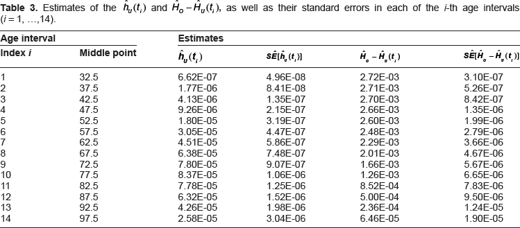
By neglecting the time-period and birth-cohort effects, we obtained ${\widehat{h}}_U\left(t_i\right)$ and $S\widehat{E}\left[{\widehat{h}}_U\left(t_i\right)\right]$ by formulas (25) to (27). Note, in our calculations, the index, i, varied from i = 1, which corresponds to the age interval with a midpoint of 32.5 years, to i = n = 14, which corresponds to the age interval with the midpoint of 97.5 years. The obtained values of ${\widehat{h}}_U\left(t_i\right)$ and $S\widehat{E}\left[{\widehat{h}}_U\left(t_i\right)\right]$ are presented in Table 3. For ${\widehat{H}}_o$ and $S\widehat{E}\left[{\widehat{H}}_o\right]$ we obtained the values of 2.72 · 10⁻³ and 2.25 · 10⁻⁵, correspondingly. The differences between the overall cumulative hazard, H_O, and the cumulative hazard function, H_U(t_i), and the standard errors of these differences are given in the third and fourth columns of Table 3.

Table 3.

Estimates of the ${\widehat{h}}_U\left(t_i\right)$ and ${\widehat{H}}_o-{\widehat{H}}_U\left(t_i\right)$ , as well as their standard errors in each of the i-th age intervals (i = 1, …, 14).

Age interval		Estimates
Index i	Middle point	${\widehat{h}}_U\left(t_i\right)$	$S\widehat{E}\left[{\widehat{h}}_U\left(t_i\right)\right]$	${\widehat{H}}_o-{\widehat{H}}_U\left(t_i\right)$	$S\widehat{E}\left[{\widehat{H}}_o-{\widehat{H}}_U\left(t_i\right)\right]$
1	32.5	6.62E-07	4.96E-08	2.72E-03	3.10E-07
2	37.5	1.77E-06	8.41E-08	2.71E-03	5.26E-07
3	42.5	4.13E-06	1.35E-07	2.70E-03	8.42E-07
4	47.5	9.26E-06	2.15E-07	2.66E-03	1.35E-06
5	52.5	1.80E-05	3.19E-07	2.60E-03	1.99E-06
6	57.5	3.05E-05	4.47E-07	2.48E-03	2.79E-06
7	62.5	4.51E-05	5.86E-07	2.29E-03	3.66E-06
8	67.5	6.38E-05	7.48E-07	2.01E-03	4.67E-06
9	72.5	7.80E-05	9.07E-07	1.66E-03	5.67E-06
10	77.5	8.37E-05	1.06E-06	1.26E-03	6.65E-06
11	82.5	7.78E-05	1.25E-06	8.52E-04	7.83E-06
12	87.5	6.32E-05	1.52E-06	5.00E-04	9.50E-06
13	92.5	4.26E-05	1.98E-06	2.36E-04	1.24E-05
14	97.5	2.58E-05	3.04E-06	6.46E-05	1.90E-05

Figure 1 shows the discrete distribution of ${\widehat{h}}_U\left(t_i\right)$ in aging (presented by circles) with the 95% confidence intervals (CI) presented by error bars. As can be seen from this Figure, the hazard rates on the population level fall in old age and has a reverse bathtub shape.

Figure 1.

Discrete distribution of the estimates of the unconditional hazard function, ${\widehat{h}}_u\left(t_i\right)$ (in person years), of pancreatic cancer in the age intervals, t_i.

Procedure 3

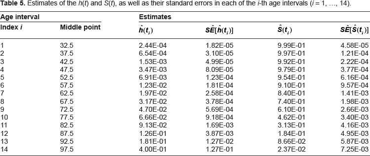
The $\widehat{f}\left(t_i\right),\widehat{F}\left(t_i\right),\widehat{h}\left(t_i\right)$ and $\widehat{S}\left(t_i\right)$ were obtained by formulas (28), (32), (34), and (40), correspondingly, while their standard errors were obtained by formulas (31), (33), (36), and (42). The obtained values of the $\widehat{f}\left(t_i\right),S\widehat{E}\left[\widehat{f}\left(t_i\right)\right],\widehat{F}\left(t_i\right),S\widehat{E}\left[\widehat{F}\left(t_i\right)\right],\widehat{h}\left(t_i\right),S\widehat{E}\left[\widehat{h}\left(t_i\right)\right],\widehat{S}\left(t_i\right)$ and $S\widehat{E}\left[\widehat{S}\left(t_i\right)\right]$ are presented in Tables 4 and 5, correspondingly.

Table 4.

Estimates of the $\widehat{f}\left(t_i\right)$ and $\widehat{F}\left(t_i\right)$ , as well as their standard errors in each of the i-th age intervals (i = 1, …, 14).

Age interval		Estimates
Index i	Middle point	$\widehat{f}\left(t_i\right)$	$S\widehat{E}\left[\widehat{f}\left(t_i\right)\right]$	$\widehat{F}\left(t_i\right)$	$S\widehat{E}\left[\widehat{F}\left(t_i\right)\right]$
1	32.5	2.43E-04	1.83E-05	6.09E-04	4.58E-05
2	37.5	6.52E-04	3.14E-05	2.85E-03	1.21E-04
3	42.5	1.52E-03	5.11E-05	8.28E-03	2.22E-04
4	47.5	3.40E-03	8.40E-05	2.06E-02	3.77E-04
5	52.5	6.60E-03	1.29E-04	4.56E-02	6.16E-04
6	57.5	1.12E-02	1.89E-04	9.01E-02	9.57E-04
7	62.5	1.66E-02	2.55E-04	1.60E-01	1.41E-03
8	67.5	2.35E-02	3.36E-04	2.60E-01	1.98E-03
9	72.5	2.87E-02	4.09E-04	3.90E-01	2.66E-03
10	77.5	3.07E-02	4.67E-04	5.38E-01	3.40E-03
11	82.5	2.86E-02	5.18E-04	6.87E-01	4.16E-03
12	87.5	2.32E-02	5.91E-04	8.16E-01	4.95E-03
13	92.5	1.56E-02	7.38E-04	9.13E-01	5.87E-03
14	97.5	9.50E-03	1.12E-03	9.76E-01	7.25E-03

Table 5.

Estimates of the h(t) and S(t), as well as their standard errors in each of the i-th age intervals (i = 1, …, 14).

Age interval		Estimates
Index i	Middle point	$\widehat{h}\left(t_i\right)$	$S\widehat{E}\left[\widehat{h}\left(t_i\right)\right]$	$\widehat{S}\left(t_i\right)$	$S\widehat{E}\left[\widehat{S}\left(t_i\right)\right]$
1	32.5	2.44E-04	1.82E-05	9.99E-01	4.58E-05
2	37.5	6.54E-04	3.10E-05	9.97E-01	1.21E-04
3	42.5	1.53E-03	4.99E-05	9.92E-01	2.22E-04
4	47.5	3.47E-03	8.09E-05	9.79E-01	3.77E-04
5	52.5	6.91E-03	1.23E-04	9.54E-01	6.16E-04
6	57.5	1.23E-02	1.81E-04	9.10E-01	9.57E-04
7	62.5	1.97E-02	2.58E-04	8.40E-01	1.41E-03
8	67.5	3.17E-02	3.78E-04	7.40E-01	1.98E-03
9	72.5	4.70E-02	5.69E-04	6.10E-01	2.66E-03
10	77.5	6.66E-02	9.18E-04	4.62E-01	3.40E-03
11	82.5	9.13E-02	1.69E-03	3.13E-01	4.16E-03
12	87.5	1.26E-01	3.87E-03	1.84E-01	4.95E-03
13	92.5	1.81E-01	1.27E-02	8.66E-02	5.87E-03
14	97.5	4.00E-01	1.27E-01	2.37E-02	7.25E-03

To perform modeling of pancreatic cancer hazards in aging, we used the multiple mutation carcinogenic model, according to which the cancer occurrence in aging on the individual level can be represented with a two- or three-parameter Weibull pdf, described by formulas (45) and (46), correspondingly. Our numerical experiments suggested that, in the case of pancreatic cancer, the best fitting of the observed data can be achieved by using the three-parameter Weibull pdf. Therefore, we show the results of this modeling below (data for two-parameter Weibull pdf are not shown).

To estimate the λ, r, and A parameters of the three-parameter Weibull pdf, we used the system of conditional equations, presented by formulas (51) to (54). By varying the values of the A from 0 to 30 years with a one-year age interval, we obtained estimates of two other parameters. For each set of parameters obtained in such a way, we evaluated the quality of fitting using the AIC as described previously. Figure 2 shows a variation of the AIC (presented by open circles) with age.

Figure 2.

Variation of the AIC with the age (in years) for the three-parameter Weibull pdf modeled function, fitted by the estimates, $\widehat{f}\left(t_i\right)$ .

As can be seen from Figure 2, the best fitting was achieved for $\widehat{A}=17$ , when AIC reached the minimum value. For this case, we found that $\widehat{\lambda }=3.55\cdot {10}^{-10}\left({\widehat{\lambda }}_l=3.21\cdot {10}^{-10};{\widehat{\lambda }}_u=3.94\cdot {10}^{-10}\right)$ ; and $\widehat{r}=5.24\left({\widehat{r}}_l=5.21;{\widehat{r}}_u=5.27\right)$ where 95% confidence intervals (CI) are given in parenthesis. The obtained values of the model parameters suggest that age of pancreatic cancer presentation has a time shift about 17 years ( $\widehat{A}=17$ ), and the average number of clones developed from the mutated cells during the first year after the beginning of the effective exposure period is $\widehat{\lambda }=3.55\cdot {10}^{-10}$ , as well as that for pancreatic cells at least five mutations are needed to became malignant ( $\widehat{\lambda }=5.24$ ).

Figure 3 shows the discrete distribution of $\widehat{f}\left(t_i\right)$ (presented by open circles and error bars presenting their 95% CI) in aging. The solid line shows the Weibull curve, obtained by using $\widehat{A}=17,\widehat{\lambda }=3.55\cdot {10}^{-10}$ and $\widehat{r}=5.24$ , which provide the best fit of the Weibull curve with $\widehat{f}\left(t_i\right)$ . As can be seen from this figure, the pdf on the individual level has a reverse bathtub shape, which is similar to the shape of the hazard rates on the population level.

Figure 3.

Discrete distribution of f(t_i), of pancreatic cancer in the age intervals, t_i, obtained from the observed pancreatic cancer incidence rates and modeled by three-parameter Weibull pdf, $f\left(\widehat{\lambda },\widehat{r};t\right)=\widehat{\lambda }\widehat{r}{\left(t-\widehat{A}\right)}^{\widehat{r}-1}\exp [-\widehat{\lambda }{\left(t-\widehat{A}\right)}^r$ .

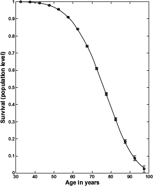
Figures 4 and 5 show the estimates (presented by open circles) of the hazard and survival functions on the individual level, obtained from the formulas (19) and (20) by substitution of the h_U(t), H_U(t) and H_O by their discrete estimates. The solid lines show the modeled hazard and survival functions with $\widehat{A}=17,\widehat{\lambda }=3.55\cdot {10}^{-10}$ and $\widehat{r}=5.24$ .

Figure 4.

Discrete distribution of the estimates of the conditional hazard function for pancreatic cancer (individual level), $\widehat{h}\left(t_i\right)$ (shown by open circles), in the age intervals, t_i, and their 95% CI (shown by the error bars).

Figure 5.

Discrete distribution of the estimates of the conditional survival function for pancreatic cancer (individual level), $\widehat{S}\left(t_i\right)$ , (shown by open circles), in the age intervals, t_i, and their 95% CI (shown by the error bars).

Notes

The h(t_i) distribution was obtained from the observed pancreatic cancer incidence rates and modeled by three-parameter Weibull hazard function, $h\left(\widehat{\lambda },\widehat{r},\widehat{A};t\right)=\widehat{\lambda }\widehat{r}{\left(t-\widehat{A}\right)}^{\widehat{r}-1}$ ; the last point of this distribution (at the age interval t₁₄ = 97.5 year) is omitted because of a very large error bar. The $\widehat{S}\left(t_i\right)$ distribution was obtained from the observed pancreatic cancer incidence rates and modeled by three-parameter Weibull survival function, $S\left(\widehat{\lambda },\widehat{r},\widehat{A};t\right)=\exp \left[-\widehat{\lambda }{\left(t-\widehat{A}\right)}^{\widehat{r}}\right]$ .

As can be seen from these figures, the modeled functions provide excellent fittings to the estimated values of the hazard and survival functions on the individual level.

Comparison of Figures 1 and 4 showed that the trends of the hazards in aging on the population level (see Fig. 1) and on the individual level (see Fig. 4) are dramatically different. Such phenomena can be explained by the fact that cancer is a rare disease occurring in the dichotomous population, a very small part of which will eventually get the cancer, while the biggest part of the population will not get cancer.

Conclusion

This work was inspired by the fact that the existing approaches used in carcinogenic modeling are focused on the ongoing processes on the individual level, while the observed data used in this modeling are obtained on the population level. Currently used mathematical equations relating hazard functions on the individual level with hazard functions on the population level are rather arbitrary, do not have clear biological/epidemiological meaning, and do not allow one to obtain an appropriate fitting with the observed data. Particularly, these equations do not answer why the hazard functions on the population level fall at old ages, while the hazard functions on the individual level do not fall.

In this work we analyzed the relationships between cancer hazards on the population and individual levels using mathematical concepts (the hazard function, h(t), the probability density function, f(t), the survival function, S(t), and frailty, α) in survival analysis. We showed that these concepts can be adopted for analyzing the hazards of cancer occurrence in aging, assuming that the considered population is a dichotomous one: a small part of this population (the fraction at risk) will eventually get the cancer, while the other part will not. We assumed that for individuals within the dichotomous population, αhas the Bernoulli distribution, with parameter p. We used the model, h_U(t) = pf(t), which is a special boundary case (when p < 1) of the general model with the Bernoulli frailty, S_U(t) = 1 – p + pS(t). It should be mentioned that an analogous model was widely used in the cure models of survival analysis, ²⁶ in which parameter pand parameters of survival function, S(t), have to be simultaneously estimated by multivariate regression. However, we showed that in the considered boundary case (p < 1), for arbitrary (parametric or non-parametric) f(t), pis equal to the overall hazard, H_O, and for estimating pit is not a necessity to perform simultaneous estimation of the parameters of the individual level survival function, S(t), by multivariate regression. This allowed us to obtain three basic equations relating the unconditional (determined on population level) hazard function, h_U(t), cumulative hazard function, H_U(t), and overall cumulative hazard, H₀, with the corresponding conditional equations (determined on the individual level) functions, h(t), f(t), and S(t), for individuals belonging to the fraction at risk: (1) h_U(t)/[H₀ – H_U(t)] = h(t); (2) h_U(t)/H₀ = f(t); and (3) [H₀ – H_U(t)]/H₀ = S(t).

One of the main advantages of these basic equations is that they have clear epidemiological meaning. Specifically, the equation h_U(t)/H₀ = f(t) indicates that the values of the hazard functions on the population level, h_U(t), are proportional to the probability density function, f(t), on the individual level, suggesting that the shapes of these functions should be similar. In addition, in this equation, the coefficient of proportionality is the cumulative hazard, H₀, that characterizes both the fraction at risk in the dichotomous population and the probability, p, that an individual will eventually get the cancer. At the same time, the other equation, h_U(t)/[H₀ – H_U(t)] = h(t), indicates that the relationship between cancer hazards on population and individual levels depends on the age and may have different shapes. This explains why the hazard functions on the population level fall at old ages, while the hazard functions on the individual level may not fall.

Using the derived basic equations, we developed a computing framework for estimating the carcinogenic parameters from the observed cancer incidences in aging. The framework includes three procedures. The first procedure is aimed at correcting the cancer incidence rates observed on the population level on the time-period and birth-cohort effects and estimating the corresponding cancer hazards in aging (on the population level). For assessing the cancer hazards in aging, this procedure uses the LLAPC model. In the present work, we have used the procedure developed in our previous work that reduces the problem of estimating cancer hazards in aging to the problem with removable interactions. ¹⁹ The second procedure is aimed at estimating in a discrete form the pdf, cdf, hazard function, and survival function on the individual level from the cancer hazards in aging estimated by the first procedure. Finally, the third procedure is aimed at determining the model parameters of the pdf from the discrete estimates of the pdf (or cdf, or hazard function, or survival function) on the individual level, performed by the previous procedure. We showed that, in a general case, this problem can be solved by methods of nonlinear regression analysis.

As an example, we estimated the modeled parameters of pancreatic carcinogenesis, using the corresponding data collected by SEER9 registries from 1975 through 2004. We showed that, in the case of pancreatic cancer, the time-period and birth-cohort effects can be neglected. Therefore, we could use the observed incidence rates as the cancer hazards in aging. Then, using the obtained cancer hazards in aging, we estimated the pdf of pancreatic cancer in a discrete form. To obtain values of the carcinogenic parameters, we used the three-parameter Weibull pdf, suggested by the Armitage-Doll multiple mutation model. By using a special technique, we reduced the nonlinear problem of estimating three parameters of the Weibull pdf, to the problem with removable interactions and estimated parameters of this pdf that provide an excellent fitting with the observed data. The estimated values of these parameters suggest that age of pancreatic cancer presentation has a time shift about 17 years, and that, for pancreatic cells, at least five mutations are needed to become malignant. Our finding of the number of mutations required for pancreatic cells to become malignant is consistent with what is known about the required number of mutations leading to cancer occurrence in other organ sites. ²⁷

Overall, in this work we mathematically proved that a simple assumption of a rareness of cancer in a dichotomous population (the Bernoulli frailty effect) is enough to explain why the observed incidence rates (hazard functions) on the population level fall at old ages, when the modeled hazard functions on the individual level are not falling. We derived three basic equations that relate the observed cancer hazards in aging on the population level with the hazard function, the pdf, the cdf, and the survival function on the individual level. We used these equations to develop a novel computing framework for estimating the carcinogenic parameters from the observed cancer incidences in aging. We suggest that the basic equations and computing framework developed in this work can be applied for estimating parameters of carcinogenic models with any given hazard function (or the pdf, or the cdf, or the survival function) on the individual level.

Author Contributions

Conceived and designed the experiments: TM, SS. Analysed the data: TM, SS. Wrote the first draft of the manuscript: TM, SS. Contributed to the writing of the manuscript: TM, SS. Agree with manuscript results and conclusions: TM, SS. Jointly developed the structure and arguments for the paper: TM, SS. Made critical revisions and approved final version: TM, SS. All authors reviewed and approved of the final manuscript.

Funding

This work was supported by the 5 R01 CA140940-03 (NIH, SS the PI) grant.

Competing Interests

Author(s) disclose no potential conflicts of interest.

Disclosures and Ethics

As a requirement of publication author(s) have provided to the publisher signed confirmation of compliance with legal and ethical obligations including but not limited to the following: authorship and contributorship, conflicts of interest, privacy and confidentiality and (where applicable) protection of human and animal research subjects. The authors have read and confirmed their agreement with the ICMJE authorship and conflict of interest criteria. The authors have also confirmed that this article is unique and not under consideration or published in any other publication, and that they have permission from rights holders to reproduce any copyrighted material. Any disclosures are made in this section. The external blind peer reviewers report no conflicts of interest.