Network-Constrained Group Lasso for High-Dimensional Multinomial Classification with Application to Cancer Subtype Prediction

Abstract

Classic multinomial logit model, commonly used in multiclass regression problem, is restricted to few predictors and does not take into account the relationship among variables. It has limited use for genomic data, where the number of genomic features far exceeds the sample size. Genomic features such as gene expressions are usually related by an underlying biological network. Efficient use of the network information is important to improve classification performance as well as the biological interpretability. We proposed a multinomial logit model that is capable of addressing both the high dimensionality of predictors and the underlying network information. Group lasso was used to induce model sparsity, and a network-constraint was imposed to induce the smoothness of the coefficients with respect to the underlying network structure. To deal with the non-smoothness of the objective function in optimization, we developed a proximal gradient algorithm for efficient computation. The proposed model was compared to models with no prior structure information in both simulations and a problem of cancer subtype prediction with real TCGA (the cancer genome atlas) gene expression data. The network-constrained mode outperformed the traditional ones in both cases.

Introduction

In cancer diagnosis, cancer patients with the same diagnostic profile may have different clinical outcomes. The difference probably lies in the limitation of the traditional classification of tumor types, based mainly on morphology. A reliable and precise classification of tumors is essential for successful diagnosis. ¹ Modern sequencing and microarray technology have enabled more detailed molecular characterization of cancer samples, leading to the discovery of many cancer subtypes. Depending on the subtype, different treatments are administered. In fact, cancer subtype identification has become an integral part of personalized medicine. ¹

Traditionally, the problem of cancer subtype classification has been approached in many ways such as multinomial logit models, ² Bayesian probit models,^3,4 random forest, ⁵ and support vector machine (SVM).^6–9 Other discriminatory methods, including linear discriminant analysis (LDA), k-nearest-neighbor (kNN) classifier, and classification trees, were also investigated. ¹⁰ Among these, SVM is a successful procedure applied to microarray-based cancer diagnosis problems.^2,11 However, it suffers from the difficulty to interpret the resulted model as well as no direct outcome probability estimates produced.^12–14 Multinomial logit model, on the other hand, is endowed with feature interpretability and probabilistic nature. ¹⁵

Classic multinomial logit model works well when the number of predictors is small. As the number of predictors increases, the generalization power of the model deteriorates because of model overfitting. When the number of predictors exceeds the number of observations as is commonly seen in genomic studies, the method breaks down. To deal with the curse of high dimensionality as well as to increase the model interpretability, regularized procedures that incorporate a sparsity penalty have been proposed.^16–20 Among these methods, group lasso is particularly appropriate for models with multiclass responses, in which all the coefficients linked to a common predictor form a group and are required to shrink to zero simultaneously in order to achieve the selection of predictors. ¹⁶

Although the sparse multinomial logit models are capable of selecting variables, they cannot efficiently use underlying structure information such as a network of regulatory relationships between genes or gene-products. Such structure information could be obtained by a data-driven approach via clustering ²¹ or other similarity-based methods,^22,23 or be extracted from the external databases accumulated through years of biomedical research. Databases such as KEGG, Reactome, and MIPS have been developed to organize different types of biological network information. Cancer is a complex disease caused by dysregulation of pathways instead of a single gene.^24–26 Thus, the incorporation of the network information can potentially increase the power of identifying cancer subtypes.

Networks are often represented as graphs, with each vertex indicating a gene or a gene-product and each edge indexed by a relationship between two vertices. Incorporation of network information has been studied in other regression models. A constraint, induced by the Laplacian matrix of the graph, ²⁷ has been proposed to facilitate the selection of predictors in ordinary regression settings, enhancing both the global smoothness over the network and the interpretability of the association between selected genes and responses in the context of known biology.

In this paper, we propose a network-constrained sparse multinomial logit model for high-dimensional multinomial classification, aiming at improving prediction performance by utilizing the underlying network prior. The remainder of this article is organized as follows. The model is first presented, followed by the algorithm to fit the model. We then validate our network-constrained model using simulations. Finally, the model is applied to a real data set of predicting the subtypes of glioblastoma multiforme (GBM).

Multinomial Logit Model and Penalized likelihood Approach

For data (y _i , x _i ), i = 1, …, n with n observations and p predictors, y _i denotes an observation of the categorical response variable Y ∊ {1, …, k} and x _i = (x_i1, x_i2, …, x _ip ) ∊ R^p indicates an observation of a p-dimensional vector of predictors. Assuming that y _i follows a multinomial distribution, a multinomial logit model is built with logit link, which is

$${\pi }_{ir}=P\left(Y=r|x_i\right)=\frac{\exp ({\beta }_{r0}+x_i{\beta }_{r.}^T)}{{\sum }_{s=1}^k\exp ({\beta }_{s0}+x_i{\beta }_{s.}^T)}=\frac{\exp ({\eta }_{ir})}{{\sum }_{s=1}^k\exp ({\eta }_{is})}$$

(1)

where β _r . = (β_r1, β_r2, β _rp ) and ${\eta }_{ir}={\beta }_{r0}+x_i{\beta }_r^T$ . We choose category k as the reference category by setting β_k0 = 0 and β_k. = 0. Under this choice, the linear predictors η_ir, r = 1, …, k−1, correspond to the log odds ratio between category r and the reference category k.

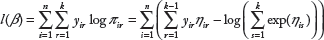
We regularize the multinomial logit model using a penalized likelihood approach, in which one maximizes the penalized log-likelihood

$$l_p\left(\beta \right)=l\left(\beta \right)-\lambda J\left(\beta \right),$$

(2)

over a (k − 1) × (p + 1)-dimensional parameter vector β = (β₁₀,…, β_(k−1)0, β_1., …, β_k−1,.) ^T . In Equation (2),

$$l(\beta )=\sum _{i=1}^n\sum _{r=1}^k{y}_{ir}\log {\pi }_{ir}=\sum _{i=1}^n\left(\sum _{r=1}^{k-1}{y}_{ir}{\eta }_{ir}-\log \left(\sum _{s=1}^k\exp ({\eta }_{is})\right)\right)$$

is the ordinary log-likelihood of a multinomial logit model, and J(β) is a function penalizing the magnitude of the parameters and regularizing the structure of features. λ, the regulatory parameter, controls the strength of the regularization.

Assuming that all predictors are metric and standardized, that is, each predictor has one degree of freedom, and the differences in scale will not influence the penalty and, thus, the variable selection. In the multinomial logit model, we use a vector β. _j = (β_1j, β_2j, …, β_k−1j) ^T of parameters to capture the effect of variable x_j, so that variable selection is achieved only when the k − 1 parameters shrink to zero simultaneously. Since the ordinary lasso facilitates only parameter selection rather than predictor selection, a group lasso penalty is utilized to penalize the parameters at a group level, defined as

$$J_1(\beta )=\sum _{j=1}^p{\varphi }_j\parallel \beta {.}_j\parallel =\sum _{j=1}^p{\varphi }_j{({\beta }_{1j}^2+{\beta }_{2j}^2+\cdots +{\beta }_{k-1j}^2)}^{1/2},$$

(3)

where ϕ _j is a penalty weight, set as 1 by default. In group lasso, all the parameters in a group β. _j would shrink to zero simultaneously.

In an association study, the graphs or networks depicting relationships among predictors are informative, supplementary to numerical data. Consider a network represented by a weighted graph G = (V, E, W) with the set of vertices V = 1, …, p corresponding to p predictors, the set of edges E = {(j, k): j and k are linked}, and the set of weights W = {w _jk : (j, k) ∊ E}. w _jk measures the level of concordance of predictors j and k, with 1 for identity and 0 for complete difference, if normalized to the scale of [0,1]. We then construct an adjacency matrix A by

$$a_{jk}=\{\begin{array}{cc}{w}_{jk}& (j,k)\in E,\\ 0& (j,k)\notin E.\end{array}$$

and a degree matrix D = diag(d₁, d₂,…,d _p ), where $d_j={\Sigma }_{(j,k)\in E}{w}_{jk}$ is defined as the degree of vertex j. The Laplacian matrix associated with graph G is L = D − A, which is always non-negative definite and can be factorized as L = SS^T. By simple algebra, ${\beta }_{r.}L{\beta }_{r.}^T$ can be written as

$${\beta }_{r.}L{\beta }_{r.}^T=\sum _{(j,k\in E)}{({\beta }_{rj}-{\beta }_{rk})}^2{w}_{jk}.$$

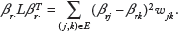
Thus, the network-constrained penalty,^22,27,28 defined as

$$J_2(\beta )=\sum _{r=1}^{k-1}{\beta }_{r.}L{\beta }_{r.}^T,$$

(4)

induces a smooth solution of the vector β_r. with respect to the labeled weighted graph G.

Typically, the adjacency matrix can be constructed from external information using the abovestated method. However, several data-driven methods are also applicable.^22,23 Adjacency coefficients can be defined based on similarity measures such as Pearson correlation coefficient, which are transformed into adjacency by a monotonically increasing function. The most widely used transformation functions include the Signum function, the sigmoid function, and the power function. Detailed examples of adjacency measures are provided by Huang and Ma. ²²

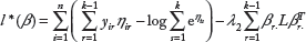
To sum up, in our regularized model, the penalized log-likelihood function is given by

$$l_p\left(\beta \right)=l\left(\beta \right)-\lambda J\left(\beta \right)$$

(5)

$$=\sum _{i=1}^n\left(\sum _{r=1}^{k-1}{y}_{ir}{\eta }_{ir}-\log \sum _{s=1}^k{e}^{{\eta }_{is}}\right)-{\lambda }_1\sum _{j=0}^p{\varphi }_j\Vert \beta {.}_j\Vert -{\lambda }_2\sum _{r=1}^{k-1}{\beta }_{r.}L{\beta }_{r.}^T,$$

(6)

of which the second term, the sparse penalty, induces model sparsity and the third term, the network penalty, imposes smoothness over the network. When λ₂ = 0, the model reduces to the group lasso multinomial logit model. The incorporation of this extra tuning parameter expands the parameter search space and directs the search to more biological meaningful regions.

Like ordinary lasso, group lasso also suffers from an issue of estimation bias, which is resulted from the fact that all predictors are penalized to the same degree. In order to reduce the bias, we use adaptive group lasso, which penalizes predictors to different degrees by assigning a weight to each predictor. In our model, the weight is set to be the reciprocal of the L₂ norm of the fitted coefficients in univariate analysis, where we fit the model with each individual predictor only. Denoting $\tilde{\beta }{.}_j$ as the univariate estimate, the group lasso penalty term (3) becomes

$$J_1(\beta )=\sum _{j=1}^p\frac{1}{\parallel \tilde{\beta }{.}_j\parallel }\parallel \beta {.}_j\parallel .$$

Proximal Gradient Method and Model Fitting

We use the proximal gradient-based FISTA (fast iterative shrinkage-thresholding algorithm) to fit the model.^29,30 Consider the optimization of the general penalized log-likelihood l _p (β) = l^*(β) − λ₁J₁ (β), composed of a concave and continuously differentiable term l^*(β), and a convex penalty term J₁ (β). The penalized maximum likelihood (ML) estimator is defined by

$$\widehat{\beta }=\underset{\beta \in R^d}{\arg \max }{l}_p(\beta )=\underset{\beta \in R^d}{\arg \max }(-1*(\beta )+{\lambda }_1{J}_1(\beta )),$$

(7)

where

$$l*(\beta )=\sum _{i=1}^n\left(\sum _{r=1}^{k-1}{y}_{ir}{\eta }_{ir}-\log \sum _{s=1}^k{e}^{{\eta }_{is}}\right)-{\lambda }_2\sum _{r=1}^{k-1}{\beta }_{r.}L{\beta }_{r.}^T$$

is a smooth function with respect to parameter β.

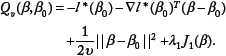
With a positive step size v, the quadratic approximation ²⁹ of −l _p (β) at a given point β₀ is

$$\begin{array}{c}{Q}_v(\beta ,{\beta }_0)=-1*({\beta }_0)-\nabla l*{({\beta }_0)}^2(\beta -{\beta }_0)\\ +\frac{1}{2v}\parallel \beta -{\beta }_0{\parallel }^2+{\lambda }_1{J}_1(\beta ).\end{array}$$

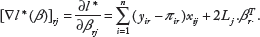
▿l^*(β), the first-order derivative of l^*(β), is a (k − 1) × (p + 1)-dimensional vector, whose element corresponding to β _rj is

$${[\nabla l*(\beta )]}_{rj}=\frac{\partial l*}{\partial {\beta }_{rj}}=\sum _{i=1}^n(y_{ir}-{\pi }_{ir})x_{ij}+2L_j.{\beta }_{r.}^T.$$

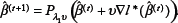
The iterations of proximal gradient methods are defined by

$$\begin{array}{c}{\widehat{\beta }}^{(t+1)}=\underset{\beta \in R^d}{\arg \min }\{-l*({\widehat{\beta }}^{(t)})-\nabla l*{({\widehat{\beta }}^{(t)})}^T(\beta -{\widehat{\beta }}^{(t)})\\ +\frac{1}{2v}\Vert {\beta -{\widehat{\beta }}^{(t)}\Vert }^2+{\lambda }_1{J}_1(\beta )\}\end{array}$$

(8)

which consists of a linear approximation of the negative modified log-likelihood at the current value ${\widehat{\beta }}^{(t)}$ , a proximity term, and the penalty term.

First, we set λ₁ = 0, and based on the standard formula for the iterates of gradient methods for smooth optimization, the unpenalized estimator ${\tilde{\beta }}^{(t+1)}$ has an explicit form

$${\tilde{\beta }}^{(t+1)}={\tilde{\beta }}^{(t)}+v\nabla l*({\tilde{\beta }}^{(t)}).$$

Then we move back to the optimization problem with an active penalty. Via Lagrange duality, Equation (7) can be equivalently expressed by

$$\widehat{\beta }=\underset{\beta \in C}{\arg \min }(-l*(\beta )),$$

where C = {β ∊ R^d|J₁(β) ≤ κ(λ)₁)} is the constraint region corresponding to J₁ (β) and κ(λ₁) is a tuning parameter that is linked to λ₁ by a one-to-one mapping. Given a search point u ∊ R^d, the so-called proximal operator associated with J₁ (β) is defined as

$$P_{{\lambda }_1}(u)=\arg {\min }_{\beta \in R^d}(\frac{1}{2}\Vert {\beta -u\Vert }^2+{\lambda }_1{J}_1(\beta$$

(9)

which is the projection of u onto region C. Then the proximal gradient iterates defined in Equation (8) can be equally expressed by the projection

$${\widehat{\beta }}^{(t+1)}=P_{{\lambda }_{1}v}\left({\widehat{\beta }}^{(t)}+v\nabla l*({\widehat{\beta }}^{(t)})\right)$$

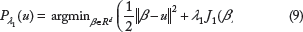
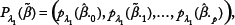
Next, consider the proximal operator (9). Owing to the block-separability of this specific penalty, the proximal operator can be written as

$$P_{{\lambda }_1}(\tilde{\beta })=\left(p_{{\lambda }_1}(\widehat{\beta }{.}_0),p_{{\lambda }_1}(\tilde{\beta }{.}_1),\cdots ,p_{{\lambda }_1}(\widehat{\beta }{.}_p)\right),$$

where

$$\begin{array}{r}{P}_{{\lambda }_1}(\tilde{\beta }{.}_0)=\underset{\beta {.}_0\in R^{k-1}}{\arg \min }\left(\frac{1}{2}\Vert {\beta {.}_0-\tilde{\beta }{.}_0\Vert }^2\right)=\tilde{\beta }{.}_0,\\ P_{{\lambda }_1}(\tilde{\beta }{.}_j)=\underset{\beta {.}_j\in R^{k-1}}{\arg \min }\left(\frac{1}{2}\Vert {\beta {.}_j-\tilde{\beta }{.}_j\Vert }^2+{\lambda }_1{\varphi }_j\parallel \beta {.}_j\parallel \right)\\ j=1,\cdots ,p.\end{array}$$

(10)

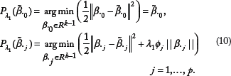
With (u)₊ = max (u, 0), the explicit solution to the proximal operator (10) can be derived from the Karush–Kuhn–Tucker conditions:

$$P_{{\lambda }_1}(\tilde{\beta }{.}_j)={\left(1-\frac{{\lambda }_1{\varphi }_j}{\Vert \tilde{\beta }{.}_j\Vert }\right)}_{+}\tilde{\beta }{.}_j,\hspace{0.17em}\hspace{0.17em}j=1,\cdots ,p.$$

Set ${\tilde{\beta }}^{(t+1)}={\widehat{\beta }}^{(t)}+v\nabla l*({\widehat{\beta }}^{(t)})$ , then the solution to the optimization problem (8) can be expressed as

$$\begin{array}{c}{\widehat{\beta }}^{(t+1)}=P_{{\lambda }_{1}v}({\tilde{\beta }}^{(t+1)})=\left(p_{{\lambda }_{1}v}(\tilde{\beta }{.}_0^{(t+1)}),p_{{\lambda }_{1}v}(\tilde{\beta }{.}_1^{(t+1)}),\cdots ,p_{{\lambda }_{1}v}(\tilde{\beta }{.}_p^{(t+1)})\right)\\ =\left(\tilde{\beta }{.}_0^{(t+1)}{\left(1-\frac{{\lambda }_1{\varphi }_j}{\parallel \tilde{\beta }{.}_1^{(t+1)}\parallel }\right)}_{+}\tilde{\beta }{.}_1^{(t+1)},\cdots ,{\left(1-\frac{{\lambda }_1{\varphi }_j}{\parallel \tilde{\beta }{.}_p^{(t+1)}\parallel }\right)}_{+}\tilde{\beta }{.}_p^{(t+1)}\right)\end{array}$$

To summarize, the basic idea of proximal gradient methods is as follows: First, remove the L₁ penalty of the objective function (6) and then optimize the smooth part by taking a step toward its ML estimator via first-order methods, which creates a search point. Second, project this search point onto the constraint region C in order to account for the non-smooth penalty term. To accelerate the convergence rate, we extrapolate the current and the previous iterations with the help of deliberately chosen acceleration factors a _t , ²⁰

$${\widehat{\alpha }}^{(t)}={\widehat{\beta }}^{(t)}+\frac{a_{t-1}-1}{a_t}({\widehat{\beta }}^{(t)}-{\widehat{\beta }}^{(t-1)}).$$

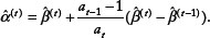
The extrapolate point ${\widehat{\alpha }}^{(t)}$ , instead of the current iterate ${\widehat{\beta }}^{(t)}$ , is used as a starting point to generate a search point, which is then projected on the penalty region.

To select the tuning parameters λ₁ and λ₂, we use cross-validation, where we divide the data set into training and test data sets. The model is trained on the training data set, and prediction error is then assessed on the test data set. We search on a grid of λ₁, λ₂ values and choose the value of λ₁, λ₂ that minimizes the cross-validated errors. The prediction error is measured with the Brier score, a measurement of the accuracy of probabilistic predictions defined as the Euclidean distance between sample response and its estimated probabilities.

Simulation

The purpose of the simulation is to show that the structure-constrained model dominates the alternative models that do not use such prior information in terms of parameter estimation and prediction. For each scenario presented, we simulate a training set and an independent test set both with 200 samples. We first select the optimal tuning parameters through a five-fold cross-validation on the training set. With the selected tuning parameters, a final model is built on the whole training set and then tested on the test set. For each setting, we run 50 simulations and calculate several criteria to evaluate the performance of the proposed model.

Simulation Settings

We consider a small model and a large model. Each model has four response categories. First of all, we construct a predictor matrix. The numbers of total predictors are 20 for small and 200 for large models, and the numbers of relevant ones are 4 and 10, respectively. The predictors are continuous and follow a multivariate normal distribution with mean 0 and the p × p correlation matrix

$$\Sigma =\left(\begin{array}{ccccc}1& \rho & {\rho }^2& \cdots & {\rho }^{p-1}\\ \rho & 1& \rho & \cdots & {\rho }^{p-2}\\ {\rho }^2& \rho & 1& \cdots & {\rho }^{p-3}\\ ⋮& ⋮& ⋮& \ddots & ⋮\\ {\rho }^{p-1}& {\rho }^{p-2}& {\rho }^{p-3}& \cdots & 1\end{array}\right),$$

where ρ = 0.5.

Second, we simulate the network structure of predictors. We divide the predictors into a few subsets (subnetworks). In the small model, 20 predictors are divided into 5 subnetworks evenly, and the 4 relevant predictors constitute the first subnetwork. In the large model, 200 predictors are divided into 20 subnetworks evenly, and the 10 relevant predictors form the first subnetwork. Ideally, we assume full connection within each subnetwork and no connection between them; that is, the corresponding adjacency matrix is a block diagonal matrix, with the main diagonal blocks being all-ones square matrices and the off-diagonal blocks zero matrices. This scenario is labeled as ideal network. We then construct the coefficient matrix, a 3 × p matrix whose rows are indexed by all but the reference categories of the response and columns are indexed by predictors. The columns corresponding to the irrelevant predictors are filled with zeros. For the relevant columns, there are three settings of the coefficients: identical, similar, and random. The first setting requires equal coefficients in each category for relevant predictors. In the case of similar coefficients, entries in each category share the same sign but have different values, indicating that all the relevant predictors impact the response in the same direction but with different magnitudes. Their absolute values are independently drawn from the set {0.05, 0.10, …, 0.50}, and the sign for each category is random. Random coefficients are independently drawn from the set {−0.50, −0.45, −0.05, 0.05, 0.50}. In this case, the prior structure information is not useful, since we assume that the coefficients within each subnetwork should be at least similar. This scenario serves as an example of model misspecification.

To further study the effects of structure misspecification, we also test our models in cases of incorrect networks and overlapping networks. In incorrect network setting, the large and small adjacency coefficients are randomly drawn from (0.4, 1) and from (0, 0.6) instead of being constant 1 and 0. In the overlapping scenario, each pair of neighboring subnetworks shares three common predictors.

Based on the multinomial logistic model, the actual probabilities can be derived and the class label is then randomly drawn from a multinomial distribution for each observation. In addition, the intercept is set to zero for the sake of a relatively balanced design.

Simulation Results

To see the improved performance of using prior structure information in terms of parameter estimation and prediction accuracy, we compare the variants of the proposed model, network-constrained multinomial logit model with group lasso penalty (NGL-MLM) and the one with adaptive group lasso penalty (NGL-MLMa), to two traditional multinomial logit models with lasso (L-MLM) and group lasso (GL-MLM), respectively, implemented in the package of glmnet in R. ¹⁶ To measure the estimation accuracy, the mean-squared error (MSE) between true parameter values and the estimated ones is used. In addition, the performance of prediction on test data is evaluated with Brier score, the Euclidean distance between sample response and the estimated probabilities, and prediction accuracy, the proportion of correctly predicted class labels.

We first simulate ideal network structure; that is, all the relevant variables come from a fully connected subnetwork. Figure 1 shows the estimation performance of various models. As expected, the structure information improves estimation significantly, especially for large models, which is particularly relevant for real applications. The estimation of the adaptive method (NGL-MLMa) outperforms others substantially. In case of random coefficients, where prior network does not provide any useful information, the proposed model is comparable to models without using the network information (L-MLM, GL-MLM), and sometimes even better. Figure 2 shows that the prediction accuracy is also higher for the proposed model in almost all scenarios. When Brier score is used (Fig. 3), a similar trend follows: the network-constrained model always performs better when we simulate ideal and similar coefficients, and is comparable to traditional models without using structure information in case of random coefficients.

Figure 1.

MSE of parameter estimation under ideal structure information for small and large models with ideal, similar, and random coefficients.

Figure 2.

Prediction accuracy rate for small and large models with ideal, similar, and random coefficients under ideal structure information.

Figure 3.

Brier scores for small and large models with ideal, similar, and random coefficients under ideal structure information.

To investigate the impact of structure misspecification, we investigate the scenarios of incorrect network and overlapping network. We simulate a medium-sized data set with 100 predictors, 10 being relevant. Each subnetwork consists of 10 predictors. For the incorrect network setting, the 10 relevant predictors come from the first subnetwork. For the overlapping network setting, the 10 relevant predictors come from two subnetworks. The performance of our models is still satisfactory because of the flexible tuning parameter on the structure-constraint term (Fig. 4). In particular, the prediction accuracy of NGL-MLM is comparable to that of GL-MLM in both situations, whereas, in terms of parameter estimation and Brier score, the structure-constrained models NGL-MLM and NGL-MLMa outperform the other two.

Figure 4.

Comparison of four candidate methods under incorrect network and overlapping network in terms of MSE, accuracy rate, and brier score.

In summary, our structure-constrained multinomial logit model has better performance in terms of parameter estimation and prediction when the prior network knowledge is at least partially correct, and the performance is comparable to traditional models when the network knowledge is incorrect. This is because the GL-MLM is a special case of NGL-MLM with λ₂ = 0. Cross-validation tends to select λ₂ = 0 when the prior assumption is not correct.

Application to the GBM Data Set

One important application of our method is cancer subtype prediction and relevant subnetwork identification on large-scale gene expression data. We apply all four candidate methods, L-MLM, GL-MLM, NGL-MLM, and NGL-MLMa, to a large-scale TCGA (the cancer genome atlas) GBM subtype prediction problem, which contains the expression data of 11,861 genes across 202 samples and four categories, with 40, 46, 58, and 58 samples in each category. The network was built from a variety of sources, including Reactome, KEGG, as well as the inferred gene-interactions from protein interactions, gene co-expressions, protein domain interactions, and text-mined interactions. The outcome is one of the four subtypes of GBM. ³¹ The data set, the network information, as well as the subtype information were downloaded from http://bioen-compbio.bioen.illinois.edu/NCIS/.

Since the number of genes in the GBM data set is much larger than the number of samples, which may lead to computation instability, we carry out gene screening before analysis. Starting with 11,861 genes, we screen genes based on the prior weights resulting from the NCIS algorithm, ³¹ by including the 599 most highly weighted genes. To construct the network smoother for model building, we tailor the original network subject to the remaining 599 genes. Then the Laplacian matrix is constructed based on the tailored subnetwork.

To compare the prediction performance of the four methods, 202 samples are randomly divided into two subsets, a training set of 150 samples and a test set of 52 samples. The random division is kept only when test samples have good representation of each category (15–35% for each category). Otherwise, we discard that division. Feature selection and parameter estimation in model building are completed strictly on the training set, and then the fitted models are tested on the test set. In practice, 50 valid divisions are obtained, and model building and testing are carried out on all pairs of data sets to assess variability, the results being summarized in Table 1.

Table 1.

Average prediction accuracy and average number of predictors in each model (model size) for the GBM data set.

	PREDICTION ACCURACY (MEAN/SD)	BRIER SCORE (MEAN/SD)	MODEL SIZE
L-MLM	0.824/0.043	3.352/0.352	52.76
GL-MLM	0.858/0.044	2.992/0.381	43.18
NGL-MLM	0.859/0.053	3.226/0.323	37.54
NGL-MLMa	0.907/0.040	2.816/0.281	34.62

The tuning parameter of the network-constraint controls the impact of the prior structure knowledge on model building. The network information will have no effect if the tuning parameter is set to zero. Among the 50 models built by NGL-MLM, the network tuning parameter is chosen as zero in 28 models, whereas NGL-MLM is reduced to GL-MLM in this specific case. In contrast, 48 NGL-MLMa models choose non-zero tuning parameter for the network-constraint, which indicates that the structure knowledge is useful for prediction, explaining the higher prediction accuracy rate for NGL-MLMa.

Next, we apply NGL-MLMa, the best model in both simulation and the application to GBM subtype analysis, on the whole sample set of GBM gene expression data and investigate the selected subnetwork. It selects 35 predictors, among which 21 are non-singletons and form a subnetwork, shown in Figure 5. The selected genes make great biological sense. For example, the most connected gene AKT1 plays an important role in the pathogenicity of GBM. AKT1 is a downstream serine/threonine kinase in the RTK/PTEN/PI3K pathway, and large-scale genomic analysis of GBM has demonstrated that this pathway is mutated in many but not all GBMs. ³² Therefore, the AKT1 can be potentially used to define GBM subtypes.

Figure 5.

The subnetwork selected by NGL-MLMa on GBM gene expression data.

Conclusion and Discussion

Cancer subtype prediction is of critical importance in the understanding, diagnosis, and treatment of cancer. We introduced a classification model on the basis of multinomial logit regression to identify cancer subtypes from high-throughput gene expression data. The model incorporates a group lasso penalty and a network-constraint. The group lasso penalizes the coefficients linked to a common predictor at a group level so that it facilitates variable selection by shrinking all elements within a group to zero simultaneously. In addition, the network-constraint improves the smoothness of coefficients with respect to the prior structure information and results in more interpretable identification of genes and subnetworks.

The proposed model and its adaptive extension are compared to lasso and group lasso multinomial logit models with no network-constraint involved. From the results of simulation and the application to GBM gene expression data, we find that the proposed model is superior given correct prior network information and is comparable to traditional models given incorrect network information.

A key challenge to the future study is to correctly specify the networks. In the application to real data, we may include too many misspecified edges on the network because of incomplete knowledge of pathways. One possible solution is to use problem-specific network for a particular type of cancer, rather than using a general molecular interaction network.

The proposed method can be extended by using a nonconvex sparsity penalty to reduce estimation bias. SCAD (smoothly clipped absolute deviation) and MCP (minimax concave penalty) are two potential candidates.^33–35 The applications of the method also go beyond the cancer subtype prediction. For example, it can also be used to predict the disease subtype based on the human microbiome data, where the phylogeny structure can be efficiently used.^28,36,37

Author Contributions

Conceived and designed the experiments: JC. Analyzed the data: XYT, JC, XFW. Wrote the first draft of the manuscript: XYT, JC. Contributed to the writing of the manuscript: XFW. Agree with manuscript results and conclusions: JC, XYT, XFW. Jointly developed the structure and arguments for the paper: JC, XYT, XFW. Made critical revisions and approved final version: JC, XYT, XFW. All authors reviewed and approved of the final manuscript.