Sage Journals: Discover world-class research

Abstract

In this study, we investigated the modalities of coding open reading frame (cORF) classification of expressed sequence tags (EST) by using the universal feature method (UFM). The UFM algorithm is based on the scoring of purine bias (Rrr) and stop codon frequencies. UFM classifies ORFs as coding or non-coding through a score based on 5 factors: (i) stop codon frequency; (ii) the product of the probabilities of purines occurring in the three positions of nucleotide triplets; (iii) the product of the probabilities of Cytosine (C), Guanine (G), and Adenine (A) occurring in the 1st, 2nd, and 3rd positions of triplets, respectively; (iv) the probabilities of a G occurring in the 1st and 2nd positions of triplets; and (v) the probabilities of a T occurring in the 1st and an A in the 2nd position of triplets. Because UFM is based on primary determinants of coding sequences that are conserved throughout the biosphere, it is suitable for cORF classification of any sequence in eukaryote transcriptomes without prior knowledge. Considering the protein sequences of the Protein Data Bank (RCSB PDB or more simply PDB) as a reference, we found that UFM classifies cORFs of ≥200 bp (if the coding strand is known) and cORFs of ≥300 bp (if the coding strand is unknown), and releases them in their coding strand and coding frame, which allows their automatic translation into protein sequences with a success rate equal to or higher than 95%. We first established the statistical parameters of UFM using ESTs from Plasmodium falciparum, Arabidopsis thaliana, Oryza sativa, Zea mays, Drosophila melanogaster, Homo sapiens and Chlamydomonas reinhardtii in reference to the protein sequences of PDB. Second, we showed that the success rate of cORF classification using UFM is expected to apply to approximately 95% of higher eukaryote genes that encode for proteins. Third, we used UFM in combination with CAP3 to assemble large EST samples into cORFs that we used to analyze transcriptome phenotypes in rice, maize, and humans. We discuss the error rate and the interference of noisy sequences such as pseudogenes, transposons, and retrotransposons. This method is suitable for rapid cORF extraction from transcriptome data and allows correct description of the genome phenotypes of plant genomes without prior knowledge. Additional care is necessary when addressing the human transcriptome due to the interference caused by large amounts of noisy sequences. UFM can be regarded as a low complexity tool for prior knowledge extraction concerning the coding fraction of the transcriptome of any eukaryote. Due to its low level of complexity, UFM is also very robust to variations of codon usage.

Keywords

genomics RNY EST ORF CDS UFM classification

Introduction

With the arrival of third generation methods for DNA sequencing, we are facing a new reality in which high-throughput sequencing is becoming affordable. This means that high-throughput data mining is necessary now more than ever.¹ With this concern in mind, the transcriptome is the first component to be addressed when approaching a new large genome, for example, that of a plant.² Because the transcriptome is the expressed part of a genome, it is a representation of the genome's coding potentialities. One must first consider that codon usage is specific to the species under investigation and is the feature that is generally considered by gene classifiers. Secondly, in prospective research, the information on codon usage for model training is not necessarily available or transferable from one species to the other. Thus, a method based on features that would allow coding open reading frame (ORF) classification independently of the codon usage is desired. This process is the same as the automatic extraction (or classification) of coding ORFs (cORF) from large samples of expressed sequence tags (EST) or full complementary DNA (cDNA) sequences. The question remains of how to automatically extract the coding component of the transcriptome to achieve high statistical significance and a low error rate, without the need for prior knowledge concerning the biological species under investigation.

Several methods for automatic extraction have previously been proposed:²³ OrfPredictor⁴ (http://proteomics.ysu.edu/tools/OrfPredictor.html) provides six-frame translation and predicts the most probable coding regions among all frames; Diogenes, which is available from the University of Minnesota (http://www.ahc.umn.edu/), identifies ORF candidates by scanning all six frames for stretches of sequences uninterrupted by stop codons, codon frequency and ORF length, which are then used to estimate the likelihood that these ORF candidates encode proteins using a quadratic discriminant function combining these various factors; ESTScan⁵ (http://www.ch.embnet.org/software/ESTScan.html) and DECODER,⁶ which are based on hidden Markov models (HMM), can detect and extract coding regions from low-quality ESTs or partial cDNAs while correcting for frame-shift errors; DIANA-EST,⁷ which is based on TIS prediction through neural network technology; and Prot4EST⁸ (http://www.compsysbio.org/lab/?q=prot4EST), which is a pipeline that predicts and translates ESTs into polypeptides using DECODER, ESTScan, and the x version of basic local alignment search tool (BLASTx).⁹

Here, we chose the universal feature method (UFM) as an investigative tool. UFM combines statistics for stop codons, ancestral codons (RNY, where R stands for a purine, N for any of the four nucleotides and Y for a pyrimidine), and base usage over six frames in a hierarchical flowchart.¹⁰ UFM's performance should not be compared with the performance of other EST processing methods^5-8 because none of these methods have a comparable cost benefit ratio. In addition, these alternative methods^5-8 require prior training or parametric adjustment of a model for a species family, whereas UFM does not. Thus, choosing the largest ORF within a transcript is the only alternative to UFM that can be used as a control to measure comparative performance. UFM is the only method that combines the stop codon density and purine bias that are both criteria specific to coding DNA and independent of biological species. The performance of UFM in the classification of introns and coding sequences (CDS) has been shown to be both better than related methods available from independent investigations and to perform at the 95% level of success rate classification, over the whole spectrum of codon usage.^10,11 Non-classified sequences (missing data) allow the evaluation of UFM classification in real situations and objective context, such as the transcriptome, which is the purpose of this study.

We found that the cORFs obtained via UFM classification of contigs from ESTs show a GC3 distribution similar to that of reference samples of CDSs. In addition, when translated into protein sequences and compared to PDB sequences using BLASTp, cORFs ≥ 300 bp produced 95% matches. These results suggest UFM can be used to extract the coding component of any transcriptome sequence set, without any previous knowledge of that species. Thus, according to the size limitation (cORFs ≥ 300 bp), UFM can be used in connection with CAP3¹² to classify cORFs from the transcriptome of any eukaryote species, without any previous knowledge of that species.

Methods

Sequence Materials and Experimental Scheme

Referencing highly confident samples of true positives becomes crucial when addressing the problem of classification optimization. To address this challenge without ambiguity, we used three strategies. First we gathered CDS samples with strong indication of being true positive, ie, ESTs homologous to the protein sequences of PDB (http://www.rcsb.org) since all accessions of PDB are: experimentally expressed, crystallized protein, and have a known function. Secondly, we gathered the EST samples among species that cover the whole range of codon usage, ie, the whole GC3 (the guanine plus cytosine content in 3rd position of codons) range of eukaryotes.^10,11 Thus, ESTs from Homo sapiens (n = 7,109,612, 30% ≤ GC3 ≤ 90%), Drosophila melanogaster (n = 820,813, 40% ≤ GC3 ≤ 85%), Oryza sativa (n=962,448, 25% ≤ GC3 ≤ 100%), Arabidopsis thaliana (n= 1,527,298, 25% ≤ GC3 ≤ 65%), Chlamydomonas reinhardtii (n=202,044, 60% ≤ GC3 ≤ 100%) and Plasmodium falciparum (n = 55,359, 0% ≤ GC3 ≤ 30%) were retrieved from GenBank (Rel. 174, Dec 14, 2009) using ACNUC.¹³ Lastly, we used the widely accepted tool of dynamic programming to establish the correspondence between an experimental sequence and its database reference. This procedure warrants a very high statistical consistency (>98%).

Samples of the EST datasets just described (queries) were compared with protein sequences (subjects) from PDB (January, 2010) in homology searches using BLASTx. The file outputs were then parsed according to their respective informative fields (query name, query size, subject name, subject size, subject definition, score, bit score, expected, identity, similarity, gaps, first base of query homology, last base of query homology, first base of subject homology, last base of subject homology) using Perl. Entries with a hit (Expected ≤ 0.0001 and Identity ≥ 40%) on the “+” strand without gaps were selected. The portion of the query sequence corresponding to the homologous region was extracted from the corresponding EST using the coordinates of the homologous region. Homologous regions with in-frame stop codons were eliminated from the sequence sample, as they could come from pseudogenes. We then built samples according to the size of homologous regions, ie, ≥100, ≥150, ≥200, ≥250 and ≥300 bp. These samples were redundant because the sample of homologous regions ≥ 100 also included homologous regions ≥ 300 bp. However, this redundancy is not a matter of concern as the aim of the experiment was to find the threshold of ORF size below which the success rate of coding ORF diagnosis would be less than 95%. The accession numbers of these samples of homologous regions of various threshold sizes were then used to retrieve the corresponding complete sequence from the original EST file. The files obtained via this process were normalized to 1,000 sequences per sample.

In this study we considered all nucleotide triplets between two stop codons as ORFs and all nucleotide triplets that could be drawn from the first 5′ in-frame ATG and the 3′ end of this ORF as ATG-Stop ORFs.

The sequences of EST regions homologous to PDB protein sequences were considered true positive CDSs, as they are expressed and contain a region that is homologous to a protein that has been crystallized (experimental data). These samples represented a convenient means of measuring the sensitivity and specificity of cORF diagnosis because the coding status and the exact position of the cORF in the sequences are known.

To find the size threshold at which a 95% success rate of cORF diagnosis occurred using the UFM classification, we set the minimum ORF size cutoff and the minimum size of the homologous regions between ESTs and protein sequences from PDB to the same value. This meant that when the EST sample contained sequences in which the region homologous to PDB was ≥100 bp, we implemented UFM with a cutoff of 100 bp; this is in contrast to when the EST sample contained sequences in which the region homologous to PDB was ≥200 bp, UFM only considered ORFs with a size ≥ 200 bp, and so on. Because the average size of ESTs homologous to PDB is rather small, samples with an average size larger than ~350 bp were not statistically consistent across all of the species addressed in this study. For this reason, UFM thresholds larger than 350 bp could not be considered for ESTs.

In order to compare the consistency of cORF sizes between species with different codon usages and species that belong to different phyla, we retrieved all CDSs of A. thaliana (n = 99,431), D. melanogaster (n=49,025) and H. sapiens (n=145,979) from GenBank using ACNUC. We then eliminated sequence redundancy with a sequence assembly program (CAP3). These sets of CDSs were considered representative of the whole gene pool of the respective species. Searching for the position of the UFM size cutoff in the cumulative size distribution of CDSs in these samples indicates the proportion of genes that is ultimately missed by UFM classification.

When the statistical parameters of cORF classification among three and six frames by UFM were established, from the samples of ESTs via reference to the coordinates of PDB homologous regions, we tested the cORF classification produced by UFM in large samples of ESTs. For this purpose, we first extracted cORFs from the complete pools of ESTs in dbEST (GenBank, rel 175) for Homo sapiens (n = 7,109,612), Oryza sativa (n = 962,448), and Zea mays (n = 2,019,105) using UFM among six frames, according a 200 bp cutoff. This cutoff clearly allowed false positives to be included, but the aim was simply to reduce the sample size and eliminate obvious non-coding ESTs. Second, we mounted contigs (EST contigs) using the resulting cORFs employing CAP3 with the default options. Third, we extracted ATG-Stop cORFs from contigs with UFM. Homo sapiens, Oryza sativa, and Zea mays were chosen because of their large GC3 heterogeneity, which allows graphical checking of false positives by comparison to the GC3 histogram of sequence frequencies and GC2 vs. GC3 scatter plots. Because potential false positives appeared in the case of humans and needed to be addressed specifically, we retrieved them (n = 1,342) using their key characteristics, ie, (i) <500 bp, (ii) GC2>(GC3+130)/3.33 and (iii) 40% ≤ GC3 ≤ 70%. We then searched for homologies among these sequences against nr (GenBank, rel 181) using the BLAST to gene ontology (Blast2GO)¹⁴ procedure with Alu sequences (alu.n.gz, available at ftp://ftp.ncbi.nlm.nih.gov/blast/db/FASTA/) and major histocompatibility complex (MHC) sequences retrieved from SRS (available at the European Bioinformatics Institute (EBI) by entering MHC in the search field (http://srs.ebi.ac.uk/srsbin/cgi-bin/wgetz?-page+srsq2+-noSession)).

The consistency of cORFs obtained from EST contigs was evaluated by comparing their GC3 distribution to those of reference samples of rice and human CDSs. In humans, the reference samples were those reported by Zoubak et al,¹⁵ since a significant amount of work on human genome organization has been carried out based on that study. At the time, genes were mostly described via experimental procedures, and the known gene number was small. Therefore, the possibility of a bias for GC-rich sequences due to the small sample size of this dataset could exist, as GC-rich genes with few or small introns were easier to sequence because of their shorter size.¹⁶ Today, most human genes have been described and their curated CDSs are available for comparative analysis. Thus, we also compared the GC3 distribution provided by Zoubak et al¹⁵ to that of the CDS sample curated by Fedorov's group (n = 23,366), which is listed in the file hs37p1.EID.tar.gz and can be downloaded from http://www.utoledo.edu/med/depts/bioinfo/database.html.^17,18 To link this CDS sample with experimental evidences, we compared the protein sequences of these CDSs with the protein sequences of PDB to determine their homology (E < 0.0001). The homologous hits were then filtered so that only the best hit was kept (n = 13,672) for each human accession. We then filtered the list, keeping pairs with an identity ≥ 40% (n = 10,892) and we used the accession identifiers to retrieve their corresponding DNA sequences from the original CDS file (n = 23,366). We considered this dataset (n = 13,672) as our sample of true positives.

The curated sample of human intron sequences (hs35p1.intrEID) that we used to measure the success rate of the CDS vs. non-CDS classification also came from Fedorov's group.^17,18 For the purpose of comparison with CDSs, in this file we only considered the first 10,348 sequences larger than 300 bp. We considered this dataset (n = 10,348) as our sample of true negatives.

In the case of rice, the reference CDS distribution was that published by Carels et al,¹⁹ which was obtained by certifying the coding status of the whole set of CDSs ≥ 600 bp from The Institute for Genomic Research (TIGR), according to the average mutual information (AMI).²⁰

Coding ORF Diagnosis

As explained above, putative cORFs were extracted from sequence samples using the UFM algorithm implemented as shown in Figure 1.

Figure 1.

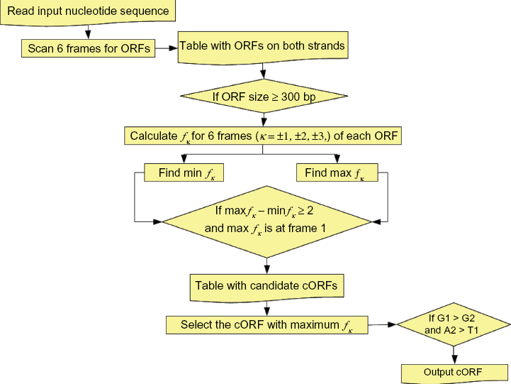
Flow chart of UFM applied to cORF finding in transcriptome sequences. f_k = P_A₍₁₎ P_G₍₁₎ I(P_C₍₁₎ P_G₍₂₎ P_A₍₃₎ + STOP + 0.01) is the UFM classifier function and is calculated over the six frames k.¹⁰

Error Evaluation

To evaluate the classification error associated with UFM, it is necessary to first consider that the error may concern 3 factors—the diagnosis of the coding status (coding or not coding), the coding strand, and the coding frame. These three components each have specific false positive, true positive, false negative, and true negative rates. Here, we explain how we measured their rate by reference to the regions of ESTs homologous to PDB protein sequences, which are considered as true positive sequences, strands, and coding frames.

The Coding Frame

If a cORF is on the same strand as the homologous region used as the true positive reference, there are 3 necessary conditions for that ORF to be considered as a true positive for the frame. First, the coordinate of the first base of the ORF must be smaller or equal to the coordinate of the first base of the homologous region because the homologous region is in frame with the coding sequence. Second, the coordinate of the last base of the ORF must be larger or equal to the coordinate of the last base of the homology detected by BLASTx. Third, there must be a whole number of nucleotide triplets (codons) between the first base of the ORF and the first base of the alignment because they must both be in frame with the coding sequence. Any ORF diagnosed as a cORF that does not obey these conditions is a false positive. False negatives correspond to the cases where a frame is diagnosed as false when it is true. This situation can only occur when a coding ORF is classified as non-coding; it is therefore a component of the false negatives with respect to coding status that are evaluated here via the success rate. The same situation occurs with true negatives.

The Coding Strand

The success rate of strand diagnosis is easy to evaluate by simply counting the number of times the strand of the homologous region matches that of the ORF (query). For example, “Plus/Plus” homologies are true positives, whereas “Plus/Minus” homologies are false positives. Again, true negatives and false negatives are part of the true negatives and false negatives regarding coding status, which was evaluated here based on the success rate of true positive detection.

The Coding Status

The rate of false negatives is given by the rate of cORFs not detected by UFM. The rate of true negative has been analyzed extensively elsewhere¹⁰ and will not be revisited here.

Finally, we evaluated the performance of UFM by comparing it to the success rates of the classification of coding sequence, strand, and frame diagnosis of the largest ORF (LORF) of the sequence considered.

At this point, we can ask what would occur when a sequence does not share a BLASTx hit with PDB. Because of the statistical distribution, we can assume that the rate of true positives, false positives, true negatives, and false negatives will be the same in this case as in the model (ORFs showing homology to PDB).

Results

Highly confident samples of true positives are necessary to test and optimize algorithms for cORF classification. The search for homologies among ESTs with PDB sequences is a simple method for this purpose. The rate of in-frame stop codon occurrence in these homologous regions of ESTs was found to be <15% in H. sapiens and was generally < 10% for the other species. The corresponding sequences were eliminated from the analysis in order to avoid an eventual bias. The cORF samples obtained via comparing ESTs with PDB protein sequences using BLASTx are presented in Table 1. The homologous regions among the sequences in these samples cover less than 40% of the entire EST set in the dbEST section of GenBank, for each of the biological species considered. This offers an interesting context in which to ask what might be the statistical significance of cORFs detected in ESTs that do not show homologous similarity to PDB sequences. However, we will first evaluate the success rate of coding frame and coding strand prediction in ESTs.

Table 1

Search of homologies between ESTs from dbEST (GenBank) with the protein sequences of PDB using BLASTx (E < 10^–4).

Species	Na^a	Hit	hit
P. falciparum	49,168	6,097 (12.4)^b	43,071 (87.6)
C. reinhardtii	20,2046	61,866 (30.6)	140,180 (69.4)
A. thaliana	49,173	14,740 (30.0)	34,433 (70.0)
O. sativa	18,0226	54,823 (30.4)	125,403 (69.6)
D. melanogaster	257,615	102,336 (39.7)	155,279 (60.3)
H. sapiens	344,064	81,281 (23.6)	262,783 (76.4)

Notes:

N is the sample size of EST sequences;

the numbers into brackets are percentages of sample size.

Coding Frame Classification when the Coding Strand is Known

Considering the success rate of coding frame detection, two situations can occur. Either the coding strand is known, for example, because the polyA tail has been detected, or the coding strand is unknown, because that information is not given.

In cases where the coding strand is known, the coding frame must be chosen from among three possibilities. The success rate of coding frame detection corresponding to such cases is given in Table 2. A 95% success rate of UFM in coding strand diagnosis (column “Bg&Phs” of Table 2) was achieved for ORF sizes ≥ 200 bp in higher eukaryotes (O. sativa, D. melanogaster, H. sapiens) and ≥150 bp in the particular case of A. thaliana. In higher eukaryotes, this level of coding strand diagnosis corresponded to a level of cORF detection (sensitivity, column “Sens” of Table 2) between 93% (H. sapiens) and 96% (D. melanogaster). For the lower eukaryotes addressed in this study (P. falciparum, C. reinhardtii), a 95% success rate of UFM in coding strand diagnosis and sensitivity was achieved for ORF sizes ≥ 100 bp.

Table 2

Success rate of coding ORF diagnosis among the three frames of ESTs of P. falciparum, C. reinhardtii, A. thaliana, O. sativa, D. melanogaster and H. sapiens for thresholds of ORF size between 100 and 300 bp. The sample size was normalized to 1,000 for each species.

Sp^a	Algorithm	Sz^b bp	Sens^c %	cORF^d, bp		Bg ≤ BgBlst^g %	End> EdBlst^h %	PhsBlstⁱ %	Bg and Phs^j %
		Sz^b bp	Sens^c %	Av^e	StDv^f	Bg ≤ BgBlst^g %	End> EdBlst^h %	PhsBlstⁱ %	Bg and Phs^j %
P. falciparum (Av: 476, StDev: 103)
	LORF¹¹	100	100.0	395	128	97.5	98.4	95.9	95.3
		150	100.0	408	120	98.7	99.3	98.0	97.8
		200	100.0	429	106	99.4	99.9	99.2	99.1
		250	100.0	447	96	99.9	100.0	99.7	99.7
		300	100.0	466	86	100.0	100.0	100.0	100.0
	UFM¹²	100	96.3	399	127	97.9	98.3	96.6	96.0
		150	97.3	411	119	98.8	99.3	98.1	98.0
		200	98.7	429	106	99.4	99.9	99.4	99.2
		250	98.1	447	96	99.9	100.0	99.8	99.8
		300	98.1	466	86	100.0	100.0	100.0	100.0
A. thaliana (Av: 485, StDev: 100)
	LORF	100	100.0	316	95	88.9	97.3	82.7	82.1
		150	100.0	323	90	92.2	99.2	88.8	88.6
		200	100.0	367	96	95.8	99.7	94.5	94.4
		250	100.0	443	109	97.8	99.9	97.2	97.2
		300	100.0	488	94	99.4	99.9	99.2	99.2
	UFM	100	85.9	323	95	95.0	98.1	91.6	91.1
		150	89.3	326	90	97.3	99.2	95.4	95.2
		200	94.0	370	97	99.0	99.7	98.0	98.0
		250	96.3	446	109	99.4	99.9	99.1	99.1
		300	98.9	488	94	99.6	99.9	99.4	99.2
O. sativa (Av: 426, StDev: 168)
	LORF	100	100.0	325	123	92.4	96.9	75.9	75.5
		150	100.0	353	116	92.6	97.6	78.4	78.3
		200	100.0	394	111	95	98.1	84.7	84.7
		250	100.0	415	95	97.5	99.4	88.4	88.4
		300	100.0	444	90	98.5	99.8	91.6	91.6
	UFM	100	89.9	323	124	95.3	97.3	90.0	89.3
		150	90.3	352	117	96.7	98.3	94.1	93.7
		200	95.1	390	112	98.1	99.2	96.8	96.8
		250	97.1	412	95	99.0	99.7	98.5	98.5
		300	98.3	441	90	99.4	99.9	99.2	99.2
D. melanogaster (Av: 537, StDev: 110)
	LORF	100	100.0	422	114	96	92.9	83.2	83.0
		150	100.0	434	109	96.9	95.5	87.2	87.1
		200	100.0	446	103	97.9	96.9	90.2	90.2
		250	100.0	470	96	98.6	98	92.2	92.2
		300	100.0	485	93	98.9	98.7	95.0	95.0
	UFM	100	93.2	424	114	96.6	94.4	89.3	88.8
		150	95.0	434	109	97.6	96.6	92.7	92.6
		200	96.4	446	104	98.4	97.9	95.1	95.0
		250	97.1	469	97	99.2	99.0	96.8	96.8
		300	98.8	484	94	99.3	99.4	97.8	97.8
H. sapiens (Av: 418, StDev: 96)
	LORF	100	100.0	299	95	90.1	96.4	80.4	79.8
		150	100.0	317	91	92.4	98.2	85.9	85.7
		200	100.0	346	84	96.5	98.9	93.5	93.4
		250	100.0	379	74	98.6	99.7	97.6	97.6
		300	100.0	413	63	99.5	100	98.7	98.7
	UFM	100	86.2	297	96	93.7	97.1	88.0	87.7
		150	88.3	315	92	95.6	98.6	92.9	92.7
		200	93.2	345	85	98.2	99.2	96.9	96.9
		250	95.2	379	74	99.0	99.9	98.8	98.8
		300	97.3	413	63	99.8	100.0	99.7	99.7
C. reinhardtii (Av: 477, StDev: 94)
	LORF	100	100.0	435	109	98.4	99.4	94.8	94.8
		150	100.0	442	105	98.4	99.6	95.6	95.6
		200	100.0	450	99	98.9	99.7	97.2	97.2
		250	100.0	473	86	98.9	99.9	97.7	97.7
		300	100.0	491	74	99.2	99.9	97.9	97.9
	UFM	100	97.6	436	107	99.8	99.8	99.6	95.4
		150	98.1	442	104	99.9	99.8	99.7	99.8
		200	98.5	450	98	99.9	99.8	99.8	99.8
		250	99.6	471	87	99.9	99.9	99.9	99.9
		300	99.8	489	75	99.9	99.9	99.9	99.9

Notes:

Sp: species name.

Sz: minimal size of homologous region in base pair.

Sens: success rate of cORF detection.

cORF: coding ORF size in base pair.

Av: average size.

StDv: standard deviation of the size.

Bg ≤ BgBlst the condition that the ORF first base is before the alignment first base.

End > EdBlst: the condition that the ORF last base is after the alignment last base.

PhsBlst: the condition that the ORF and the alignment are in the same triplet phase.

Bg and Phs: the condition that Bg ≤ BgBlst and PhsBlst are both true.

LORF: the largest ORF among the three frames.

UFM: universal feature method. Gray areas stand for the threshold of 95% statistical consistency.

In comparison to diagnosis based on the largest ORF (LORF), diagnosis using UFM appeared to be more robust and stable across species. In lower eukaryotes, the sensitivity was clearly higher for LORF, but this is associated with a lack of discrimination because this method would also find a LORF in non-coding ESTs; thus the sensitivity is deprived of meaning in the case of LORF. Regarding coding strand diagnosis, we found no significant difference between LORF and UFM, which shows that in lower eukaryotes stop codon density is a strong coding frame identifier, even in a GC-rich genome such as that of C. reinhardtii. In higher eukaryotes, LORF did not perform as well and the target success rate of coding strand diagnosis was achieved at larger ORF size. A striking case was that of rice, where the 95% success rate level was not achieved by LORF, even at 300 bp.

The average size of cORFs detected by UFM naturally increased with the cutoff threshold and was between 350 and 450 bp at the 95% success rate level, corresponding to a cutoff of 200 bp. The columns in Table 2 corresponding to “Bg≤BgBlst”, “End> EdBlst”, “PhsBlst” and “Bg&Phs” show the progression of the error. The order of these conditions in terms of decreasing success rates is as follows: “End> EdBlst” > “Bg≤BgBlst” > “PhsBlst” > “Bg&Phs”. The results show that incorrect ORFs tended to begin within homologous regions and extend over their corresponding in-frame cORFs. As would be expected, the strongest measure among was “PhsBlst”, which reports ORFs that are in the same frame as the homologous region (considered to be the true positives). However, an ORF could be located in the same frame as the homologous region, but not overlapping it. “Bg&Phs” shows that this event tends to disappear at the 95% level of consistency. We observed that the conditions “Bg&Phs” and “End>EdBlst” were redundant to the others and therefore not necessary (data not shown).

Coding Frame Classification when the Coding Strand is Unknown

In cases where the coding strand is unknown, the coding frame must be chosen from among six possibilities. The success rate of coding strand detection in such cases is given in Table 3. The trends observed in this table are similar to those of Table 2, except that the introduction of a variable corresponding to this strand introduces one additional degree of freedom. Consequently, the 95% consistency is achieved at a larger ORF size, typically 300 bp for higher eukaryotes and 150 (C. reinhardtii) to 200 bp (P. falciparum) for lower eukaryotes. The 95% consistency level for coding strand diagnosis corresponded to at least a 97% sensitivity over all species. Using LORF, the 95% consistency level for coding strand diagnosis was not achieved (even for 300 bp ORFs) in GC-rich genomes (D. melanogaster, O. sativa, H. sapiens) and only applied to GC-poor genomes, such as those with a GC content equal to that of Arabidopsis (GC ~40%) or lower. In the particular case of P. falciparum, which exhibits an extremely rich AT content, LORF was even more efficient than UFM; however, it has no discrimination power between coding vs. non-coding DNA. Comparison of UFM to LORF in the EST context shows the compensatory effect of the ancestral codon (RNY) and stop codon density on the classification of the coding status of DNA.

Table 3

Success rate of coding ORF diagnosis among the six frames of ESTs of P. falciparum, C. reinhardtii, A. thaliana, O. sativa, D. melanogaster and H. sapiens for thresholds of ORF size between 100 and 350 bp. The sample size was normalized to 1,000 for each species.

Sp^a	Algorithm	Sz^b bp	Sens^c	Strd+^d	cORF^e, bp		Bg ≤ BgBlst^h %	End> EdBlstⁱ %	PhsBlst^j %	Bg and Phs^k%	Bg and Phs and Strd^l %
		Sz^b bp	%	%	Av^f	StDv^g	Bg ≤ BgBlst^h %	End> EdBlstⁱ %	PhsBlst^j %	Bg and Phs^k%	Bg and Phs and Strd^l %
P. falciparum (Av: 508, StDv: 75.2)
	LORF¹³	100	100.0	95.3	396	126	96.7	97.5	92.7	92.3	91.6
		150	100.0	96.6	409	119	98.1	98.5	95.7	95.5	94.8
		200	100.0	98.3	429	105	99.6	99.3	98.0	98.0	97.6
		250	100.0	98.6	447	96	99.9	99.7	98.4	98.4	98.3
	UFM¹⁴	150	97.3	95.6	402	125	96.3	96.4	95.9	92.1	91.6
		200	98.7	97.1	422	110	97.4	97.6	97.8	95.5	95.2
		250	99.0	99.5	447	97	99.7	99.7	99.4	99.4	99.3
A. thaliana (Av: 485, StDv: 100)
	LORF	250	100.0	91.3	448	107	96.1	99.5	93.1	91.5	89.3
		300	100.0	95.7	489	93	98.8	99.6	97.3	96.7	95.2
		350	100.0	96.1	507	78	99.5	99.8	97.8	97.5	96.0
	UFM	250	96.7	92	434	110	95.4	96.6	97.4	94.1	91.0
		300	98.1	95.7	483	95	98.1	97.6	98.5	97.4	95.2
		350	99.8	96.2	505	78	99.1	98	99.8	98.7	95.9
O. sativa (Av: 426, StDv: 168)
	LORF	250	100.0	77.7	425	94	97.0	98.7	78.9	77.8	69.7
		300	100.0	80.3	453	93	97.6	99.2	82.4	81.5	74.7
		350	100.0	78.7	488	90	97.3	99.2	83.8	82.4	73.9
	UFM	250	97.5	92.2	406	95	97.2	97.2	96.1	94.9	91.4
		300	98.1	95.1	438	90	98.6	97.8	98.5	97.5	94.8
		350	99.1	96.7	474	84	98.2	98.7	99.5	97.6	96.5
D. melanogaster (Av: 537, StDv: 110)
	LORF	250	100.0	73.6	483	95	98.7	96.3	82.8	82.7	67.4
		300	100.0	74.1	498	92	98.9	97.2	85.2	85.1	69.7
		350	100.0	74.7	520	91	99.6	98.4	87.9	87.8	73.4
	UFM	250	97.7	94.7	463	97	98.4	97.7	97.1	96.6	92.9
		300	99.0	96.1	480	95	98.8	98.2	98.2	97.9	95.1
		350	99.4	98.3	506	91	99.5	99.1	99.0	98.4	97.1
H. sapiens (Av: 418, StDv: 96)
	LORF	250	100.0	87.9	383	73	96.6	99.1	91.2	89.7	86.4
		300	100.0	90.5	415	63	98.4	99.8	93.3	92.4	89.4
		350	100.0	92.0	448	62	98.6	99.9	94.1	93.2	91.5
	UFM	250	94.8	93	374	74	97.6	96.8	98.8	96.9	92.8
		300	97.3	95.9	410	64	98.6	98.0	99.2	98.0	95.5
		350	98.3	97.9	444	61	99.7	99.0	99.7	97.7	96.0
C. reinhardtii (Av: 477, StDv: 94)
	LORF	150	100.0	64.5	452	104	98.8	99.4	68.6	68.6	61.6
		200	100.0	65.8	458	99	99.2	99.5	70.2	70.2	63.9
		250	100.0	65.8	482	86	99.4	99.6	70.6	70.6	63.9
	UFM	100	97.2	95.7	426	116	99.0	96.5	95.9	93.2	92.7
		150	97.5	97.0	436	109	99.7	97.5	97.3	97.3	96.8
		200	98.0	99.0	449	99	99.8	99.2	99.2	99.2	98.8
		250	99.3	99.8	471	87	99.8	99.8	99.7	99.7	99.7

Notes:

Sp: species name.

Sz: minimal size of homologous region in base pair.

Sens: success rate of cORF detection.

Strd+: success rate of coding strand classification.

cORF: coding ORF size in base pair.

Av: average size.

StDv: standard deviation of the size.

Bg ≤ BgBlst: the condition that the ORF first base is before the alignment first base.

End > EdBlst: the condition that the ORF last base is after the alignment last base.

PhsBlst: the condition that the ORF and the alignment are in the same triplet phase.

Bg and Phs: the condition that Bg ≤ BgBlst and PhsBlst are both true.

Bg and Phs and Strd: the condition that Bg and Phs and the cORF is on the “+” strand are both true.

LORF: the largest ORF among the six frames.

UFM: universal feature method. Gray areas stand for the threshold of 95% statistical consistency.

Regarding the evaluation of the success rate of coding strand diagnosis, introducing one degree of freedom in the strand increases the probability of obtaining an ORF in the same phase as the homologous region, but on the opposite strand. To filter this type of event out, it is necessary to score the proportion corresponding to the condition that the two events “Bg&Phs” and having the cORF on the “+” strand (that of the region homologous to PDB, by definition) occur together, which we denoted “Bg&Phs&Strd” in column 12 of Table 3. Based on comparison of Tables 2 and 3, it is obvious that the main source of error in GC-rich species produced by LORF is from diagnosis of the coding frame on the “–” strand when it is actually on the “+” strand. This is because the largest ORF is on the “–” strand in a significant proportion of the coding DNA in these species.

We found the consistency of the 200–300 bp cutoff for cORF to be acceptable because 93%–95% of the coding sequences of higher eukaryotes (taking A. thaliana, D. melanogaster and H. sapiens as representatives, Fig. 2A) are above this threshold (Fig. 2B).

Figure 2.

Size distribution of non-redundant coding sequences (GenBank) of A. thaliana (n = 29339), D. melanogaster (n = 15578) and H. sapiens (n = 31318). The top panel (A) is for the relative frequencies and the bottom panel (B) for the cumulated relative frequencies.

Since a success rate of ≥95% true positives corresponding to a sensitivity of >97% is obtained with UFM for ORFs ≥ 300 bp in ESTs of higher eukaryotes, it begs the question of what the success rate would be when the coding status is unknown, as is the case when BLAST homologies to PDB and/or other databases are not available.

Classifying cORFs in Rice ESTs

When the UFM classification was tested on ATG-Stop cORFs (the ATG-3n-Stop coding ORFs diagnosed by UFM) from rice EST contigs (n = 16,533), we did not find any consistent difference between the profiles of the observed (plain lines in Fig. 3) and expected frequencies (dashed lines in Fig. 3) for GC3 (Fig. 3A) or GC2 vs. GC3 (Fig. 4A). The histogram (GC3) and scatter plots (GC2 vs. GC3) actually match those found using the CDS sample from TIGR, corrected by AMI filtering for false positives.¹⁹ The analysis of ATG-Stop cORFs from singlets (n = 8,068) revealed the same pattern for GC3 (Fig. 3B) and GC2 vs. GC3 (Fig. 4B), though with some possible false positives being observed in the compositional range below GC3 = 30%. Interestingly, the sum of cORFs (n = 24,600) from contigs (n = 16,533) and singlets (n = 8,068) is close to the reported gene number of approximately 25,000 for Arabidopsis.

Figure 3.

GC3 distribution of ATG-Stop cORFs (>300 bp) in the rice transcriptome. (Panel A) shows the distribution for the contigs of 962,448 ESTs from GenBank. (Panel B) shows the distribution for the singlets obtained after contig assembling.

Figure 4.

Scatter plots of GC3 vs. GC2 of ATG-Stop cORFs (>300 bp) in the rice transcriptome. (Panel A) shows the distribution for the contigs of 962,448 ESTs from GenBank. (Panel B) shows the distribution for the singlets remaining after contig assembling.

Prior Knowledge and cORF Classification in Human ESTs

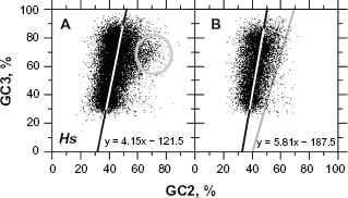
In the case of the humans, we found that the GC3 of mRNA sequences of Fedorov's group^17,18 calculated in reference with their first bases (Fig. 5A, thin line) is clearly out of frame. The GC3 calculated from their cORFs obtained with UFM (Fig. 5A and B, bold line) matched those of CDSs from that group (Fig. 5B, thin line) and from Zoubak et al¹⁵ (Fig. 5B, dashed line). Consequently, most of the mRNAs from Fedorov's group^17,18 are out of coding frame but the gene annotation is correct. The framing of mRNA by UFM (ATG-Stop ORF) is also correct. Similarly, the mismatch between the distributions of CDSs from the original dataset of Fedorov's group^17,18 and the same dataset after filtration for homology with PDB sequences was only ~2% (Fig. 6A). The mismatch between the distributions of CDSs from Fedorov's dataset^17,18 after filtration for homology with PDB sequences and that of Zoubak et al¹⁵ was in the same range, which is reassuring given the much poorer knowledge of the human genome at that time (Fig. 6B).

Figure 5.

The GC3 distribution in the reference dataset of human coding sequences. (Panel A) comparison between GC3 distribution from sequences in the hs37.mrnaEID file (mRNA), (1) GC content in 3rd position o triplets taken from the 1st base of the sequences (n = 23,315), (2) GC3 of ATG-Stop ORFs (n = 24,419) obtained with UFM. (Panel B) comparison between the GC3 distributions of reference (1) and (3) with the GC3 of ATG-Stop ORFs obtained with UFM. (1) is for the GC3 distribution of the coding sequences (n = 23,366) extracted from the gene sequences (hs37. dEID) using the coordinates given in the title lines of the fasta file, (3) is for the GC3 distribution (n = 4,270) published by Zoubak et al.¹⁵ (Panel C) Histograms of relative frequencies (%) in human CDS according to GC3 level (%). The dataset of Fedorov's group^17,18 (bold line, n = 23,366) is compared to the distribution of the CDSs from the same dataset that are homologous to PDB (gray line, n = 10,892) (the mismatch between both distributions is only ~2%). The distributions of (1), (2), (3) and (4) match almost perfectly which demonstrates that (i) the distribution by Zoubak et al¹⁵ was mostly unbiased, (ii) the dataset of Federov's group^17,18 is mostly unbiased and that UFM efficiently extract coding ORFs in their correct reading frame with unknown sample whatever their GC content.

Figure 6.

GC2 vs. GC3 scatter plots of CDSs in H. sapiens (Hs). The sequence sample curated by the Fedorov's group^17,18 (Panel A) is compared to the scatter plot of the same sequence sample after alignment with the protein sequences of PDB (Panel B).

Scatter plotting of data is a powerful method for determining outliers that may be false positives. The scatter plots presented in Figure 6 show that the mismatch between the two GC3 distributions of Figure 5C is actually due to a small number of sequences within the gray circle in Figure 6A. These sequences are not present in the scatter plot shown in Figure 6B, which suggests that they are false positives because the plot in Figure 6B is based on sequences with undisputable experimental evidence (protein crystallization) and almost no dots are found on the right side of the line y = 3.33x – 130 (Fig. 6B). This line does not participate in the UFM classification process; it is only used as a guideline to facilitate plot-to-plot comparisons.

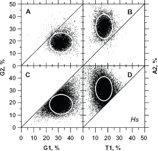
Considering the intron dataset of Fedorov's groups as representative of non-CDSs (ie, true negatives), as well as the dataset of curated CDSs from the same group that are homologous to PDB (ie, true positives) as representative of human CDSs, we determined that the classification threshold τ that generates the same rates (~11%) of false positives and false negatives (Fig. 7) took a value of 3.5 in humans when UFM was used without a posteriori filtering. Because A2 > T1 (Fig. 8A) and G1 > G2 (Fig. 8B) are generally true in the coding frame, a posteriori filtering under these conditions and a setting of τ ≥ 2 (Fig. 8C and D) decreased the rate of false positives, with no significant alteration of sensitivity (Fig. 9). However, it did not completely eliminate the false positives (as shown by the dots outside of the white ellipses and close to the diagonal in Fig. 8C and D), which is not surprising given the small difference in composition between CDSs and contiguous non-coding sequences.²¹ Filtering out these false positives should only be considered on a case-to-case basis because it would affect the universality of UFM seeing as it would affect its applicability to other species without previous knowledge. The exact position and geometry of these ellipses actually change slightly according to the average GC level of the species under consideration (data not shown).

Figure 7.

Histograms of UFM score in human introns (n = 10,348) and CDSs (n = 10,892). About 40% of introns (thin line, n = 3,346) gave UFM values larger than one.

Figure 8.

Scatter plots of G1 vs. G2 (A and C) and T1 vs. A2 (B and D) in human CDSs from Fedorov's group dataset^12,13 homologous to PDB (A and B) and cORFs (classified by UFM) from human EST contigs (C and D).

Figure 9.

Histograms of UFM score in human introns and CDSs with a posteriori filtering using A2 > T1 and G1 > G2. About 13.5% of introns (thin line, n = 1,650) gave UFM values larger than two and confused the CDS (bold line, n = 9,985) classification.

When the ATG-Stop ORFs were extracted by UFM from the contigs (n = 57,374) in the entire GenBank set of human ESTs (n=7,109,612), we found that their GC3 frequency was higher than the GC3 of CDSs on the GC-poor side of the reference distributions. When we filtered out the sequences shorter than 500 bp, the profiles of GC3 of ATG-Stop ORFs tended to match that of the reference dataset (Fig. 10C), suggesting that ~5% of false positives (the difference between the plain lines in Fig. 10A and C) fall in the range of 40% ≤ GC3 ≤ 70% for ORFs shorter than 500 bp. The difference between the plots shown in Figure 10A and C did not increase when filtering out ORFs larger than 500 bp (data not shown), suggesting that the cORFs in ~8% of the area (gray area) between thin and dashed lines in Figure 10C should indeed be considered as true positives and that the higher frequencies in the range of 40% < GC3 < 70% found for ATG-Stop ORFs compared to the reference distribution occurs simply because some GC-rich genes are expressed at lower rates than other genes. However, it is also true that for cORFs larger than 500 bp, a proportion of the cORFs outside the areas corresponding to the white ellipses in Figure 8C and D remain unchanged (data not shown), which demonstrates some of the cORFs in the 8% area (Fig. 10C) are indeed false positives. Figure 10B and D show that the ATG-Stop ORFs are much larger and that their proportion remains considerable in the 40% ≤ GC3 ≤ 70% interval of singlets, even at sizes larger than 500 bp. The fact that the frequency of ATG-Stop ORFs in singlets decreased more rapidly in the 50% < GC3 < 65% interval than in the 65% < GC3 < 75% interval (when only considering ORFs larger than 500 bp) is consistent with the hypothesis that they come from pseudogenes that are still expressed at very low levels.

Figure 10.

GC3 distribution of ATG-Stop ORFs in human transcriptome compared to the genomic reference. ATG-Stop ORFs larger than 300 bp from contigs are more frequent in the 40% ≤ GC3 ≤ 65% interval compared to the reference by –13% (A). The rate of ATG-Stop ORFs larger than 300 bp from singlets in the 40% ≤ GC3 ≤ 65% interval is at least 5 times higher than in contigs (B). The rate of ATG-Stop ORFs larger than 500 bp from contigs in the 40% ≤ GC3 ≤ 70% interval is only ~8% higher compared to the reference, but the profile of GC3 distribution parallels that of the reference showing that these –8% difference are expected to be due to a difference of expression rate between GC-rich and GC-poor genes in favor of GC-poor genes (C). The rate of ATG-Stop ORFs larger than 500 bp from singlets decreases more rapidly in the 40% ≤ GC3 ≤ 65% interval than in the 65% ≤ GC3 ≤ 75% interval (D).

The GC3 interval where we observed the most significant difference between the profiles shown in Figure 10A and C is marked by the gray arrows in Figure 11A and C. It is clearly visible from the lower density of dots in Figure 11C compared to Figure 11A in the 40% ≤ GC3 ≤ 70% range around GC2 = 55%, delimited by the line y = 3.33x – 130. Counting ~13% false positives in the 40% ≤ GC3 ≤ 70% interval, the number of human genes would be approximately 26,000 (47% of human EST contigs). However, it is impossible to calculate the proportion of singlets that could contribute to the gene number given the high noise level. Figure 11D suggests that at least 3,000 singlet cORFs could be true positives. Thus, the final expected number of true positive cORFs would be approximately 25,000–30,000, which is in agreement with the current view of the gene number in humans.

Figure 11.

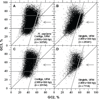
Scatter plot of GC3 vs. GC2 of ATG-Stop cORFs extracted with UFM from the human transcriptome. The gray arrow indicates the ATG-Stop ORFs from contigs larger than 300 bp that are more frequent in the 40% ≤ GC3 ≤ 70% interval and delimited by the line y = 3.33x – 130 compared to the reference (A). The ATG-Stop ORFs in the 40% ≤ GC3 ≤ 70% interval and delimited by the line y = 3.33x – 130 are also present in singlets (B). The plot of ATG-Stop ORFs from contigs larger than 500 bp shows that they disappear in the 40% ≤ GC3 ≤ 70% interval delimited by the line y = 3.33x – 130 (C). The same trend that is found in panel C with contigs is also found in singlets (D).

In comparison with rice, the higher discrepancy between the profiles of ATG-Stop ORF distributions in contigs and singlets for GC3 histogram, as well as for GC2 vs. GC3 scatter plots found in humans, suggests a higher rate of genetic load accumulation in humans than in rice. This interpretation is supported by the plot shown in Figure 12, where genetic load accumulation would be higher in maize than in rice. This is in fact expected based on the higher rate of transposon and retrotransposon activity in maize than in rice.

Figure 12.

Scatter plot of GC3 vs. GC2 of ATG-Stop cORFs extracted with UFM in maize transcriptome. The relationship of GC3 vs. GC2 from contigs is plotted in (A) while that from singlets is plotted in (B).

Searching for Functions in ORFs with a Purine Bias that are Apparently False Coding

In humans, a substantial proportion (n = 6,221) of ESTs from singlets (28,341, with nucleotides denoted as N, B, H, K, W, S, Y, and R) were of rather low quality, which make these sequences unique and hampers their assembly with the existing contigs. However, among the 28,341 singlet sequences, 22,120 did not contain an “N”, but 17,159 were <500 bp, which is a proportion that is too large (17,159/22,120 = 77.6%) to be explained by the low sequence quality (21.9%) of the sample. These sequences, which tended to be associated with the highest GC2 levels (GC2 > 50%, Fig. 11B and D), were also those where Alu elements tended to map (Figs. 13 and 14). However, the number of sequences that were homologous (E < 0.0001) to Alu elements was only 703, ie, much lower than 10,789.

Figure 13.

The GC3 distribution of ATG-Stop cORFs from contigs homologous (BLASTn, E ≤ 0.0001) to Alu elements compared to GC3 references.

Figure 14.

The GC3 vs. GC2 scatter plot of ATG-Stop cORFs from contigs homologous (BLASTn, E ≤ 0.0001) to Alu elements.

Testing MHC CDSs as another source of sequences with a possible bias, we found that these genes are indeed rich in GC2 (>40%), as observed in Figure 15A and B. However, the sample tested was out of the coding frame (ellipse of Fig. 15A) and needed to be analyzed using UFM to obtain a more reliable GC3 vs. GC2 relationship (Fig. 15B). We found that all ATG-Stop ORFs among human EST contigs homologous to MHC CDSs (BLASTn, E ≤ 0.0001) showed a GC3 content in the same range as that of GC2, suggesting their transformation in pseudogenes (Fig. 15C).

Figure 15.

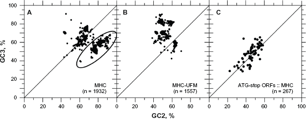
Scatter plot of GC3 vs. GC2 for MHC coding sequences. The sample of MHC coding sequences (CDS) retrieved from GenBank was found to be out of frame (black ellipse). In about half of the cases the frame + 1 has been confused with frame –3 (dots within the ellipse of Panel A). The CDSs from MHC treated with UFM have a GC3 vs. GC2 plot conform to the expectations from the human gene relationship from Figure 11 (Panel B). The homologies of ATG-Stop cORFs of human EST contigs found by BLASTn (E ≤ 0.0001) with the MHC CDSs were on the diagonal (Panel C).

Because the sequences from the singlet sample are not expressed more than one time among 7,109,612 ESTs (18,444/7,109,612 = 0.26%), it is not justified to consider them as true positives. This finding shows that the samples based on the distribution of ATG-Stop ORFs among contigs are more reliable than those based on ORFs in singlets, as the latter can be contaminated by noisy sequences.

At least some of the approximately 5% of putative false positives delimited by the line y = 3.33x – 130 in the 40% ≤ GC3 ≤ 70% range (n = 1,342) could have some biological significance, as they are expressed more than one time. By comparison to Gene Ontology (GO), we found 601 (45%) homologous sequences using BLASTx (Blast2GO, E ≤ 0.000001) against the nr database and 402 (30%) GO annotations.

These annotations could be divided into three groups. The first group consists of cellular components (Fig. 16A), with eight non-redundant groups (n = 413) on the sixth GO level, ie, organelles (66%), nuclear parts (10%), cytosol (7%), nucleolus (6%), nucleoplasm (5%), ribosome (2%), cytoplasmic vesicle (3%), and cytoskeletal parts (2%). The second group consists of biological processes (Fig. 16B), with nine non-redundant groups (n = 361) on the fifth GO level, ie, signal transduction (20%), cellular macromolecule biosynthetic processes (20%), nucleic acid metabolic processes (20%), cellular protein metabolic processes (16%), protein transport (7%), establishment of protein localization (7%), ion transport (4%), regulation of cellular component size (3%), and regulation of macromolecule metabolic processes (1%). The third group consists of molecular functions (Fig. 16C), with twelve only slightly redundant groups (n = 446) on the third GO level, ie, protein binding (43%), hydrolase activity (12%), nucleotide binding (11%), transferase activity (10%), signal transducer activity (9%), transcription factor activity (4%), ion binding (3%), lipid binding (2%), carbohydrate binding (2%), chromatin binding (2%), and transmembrane transporter activity (1%), which means that ~80% seem to be involved in binding activities.

Figure 16.

Annotation of the ATG-Stop cORFs extracted with UFM in the 45 < GC3 < 65 vs. 50 < GC2 < 60 interval of the human EST contigs. Annotations were obtained by comparing cORFs with nr using BLAST2GO. Functional categories are organized within cellular component (A), biological process (B) and molecular function (C).

Discussion

UFM is a type of decision tree²² in which a candidate coding ORF (cORF) flows across a sequence of tests involving less than 20 variables addressing objective criteria (eg, purine bias and stop codon frequency) that are the first determinants of coding DNA features. We showed above that UFM is a convenient tool for the extraction of cORFs from the transcriptome of any eukaryote. Considering the cORF classification among the six frames of CDSs homologous to the protein sequences of PDB, UFM provides an approximately 95% success rate in cORF diagnosis for approximately 95% of coding sequences (CDS) ≥300 bp in the case of higher eukaryotes. The fact that the same performance is obtained even for lower size (typically 200 bp) in Plasmodium falciparum and Chlamydomonas reinhardtii is intriguing and suggests stronger codon pressure through translation selection in lower eukaryotes. A corollary of this is that relaxed translation selection allows higher protein sequence complexity to occur, which may have consequences for the spectrum of protein functionality and UFM classification power.

The size threshold corresponding to a 95% success rate of cORF classification among ESTs can be lowered by 100 bp to 200 bp in higher eukaryotes and 100 bp in lower eukaryotes if the coding strand is known. This is the case when, for instance, the polyA tail is present or when cDNA are obtained through directional Sfi I restriction. Consequently, with a minimum technological investment, it is possible to recover most coding sequences of proteins in eukaryote transcriptomes through simple bioinformatics, without need for prior knowledge regarding the biological species or its genome structure. Because exons constitute the most reliable sequence anchorage in the genome, their detection facilitates systematic intron and promoter scanning. Adding compiled information about promoters, exons, and introns represents a necessary input for HMM models that may help to track hidden genes with a low level of expression. This suggests that UFM is suitable for making part of the first layers of an automatic system for producing genome information.

UFM allows automatic transcriptome phenotype visualization in the compositional sense given to the genome phenotype by Bernardi.²³ That is, UFM allows the fast calculation of the distribution of CDSs according to GC3, in an impromptu manner, on the output of cDNA sequencing. Recording the number of cORFs assembled in each contig provides information regarding the level of expression of the sequenced genes. Mounting contigs from cORFs of ESTs has the side effect of measuring the level of expression just by counting ESTs per contig, for example, visualizing or picturing the transcriptome phenotype also allows the RNA-Seq to be performed.^24,25

Due to the compositional transition that occurred in Gramineae²⁶ and warm-blooded vertebrates,²³ the genes of these taxa are distributed over a compositional interval that covers ~75% of the complete range of GC3 vs. GC2 variation observed across living beings (ie, the so-called universal correlation).²⁷ Information regarding the GC3 level is important because this parameter may confound gene classifiers. Knowledge of GC3 heterogeneity can also be important when addressing biological evolution in relation to compositional constraints on DNA and the structure of the ecological niche of the species under investigation. Here, we used prior knowledge of the transcriptome phenotype to aid in decision making concerning cORF reliability. Comparison of GC3 vs. GC2 plots may actually facilitate the detection of spurious putative CDSs. We considered three levels of information to determine the coding status of an ORF. Firstly, at structural level, the sequence stretch is formed by a whole number of nucleotides triplets between 2 stop codons, between an ATG and a stop codon, between an extremity and a stop codon, and between an ATG and an extremity or between two extremities. Secondly, at the base composition level, the sequence satisfies the RNY pattern, ie, a higher probability of a purine in the first codon position and a lower product of the probabilities of a CGA occurring in the coding frame. Thirdly, at the expression level, the level of expression should be higher than one EST for a given gene when the EST sample is large. In the context of an EST expressed more than one time, the largest ORF is sufficient to diagnose the potential coding frame of a cORF in the transcriptome of a GC-poor species, such as Plasmodium falciparum. The contribution of RNY is essential for cORF diagnosis at a high GC content (>60%). Due to the compensation of UFM for RNY and stop codon frequency according to the GC context, its success rate is not significantly affected by the codon usage of a given species.¹⁰

When considering plants, we found that the GC3 vs. GC2 plots of ATG-Stop cORFs from contigs match that of the universal correlation. This strongly suggests that UFM can be used on the transcriptome of any plant species for extracting cORFs, without any additional knowledge or parametric tuning. This was true even in new cases, such as for genetic prospecting for exploration of biodiversity. The same plot for ATG-Stop cORFs obtained from singlets also matches the universal correlation, except in case of maize, where the plot is contaminated by noisy sequences in the ranges of 40% ≤ GC3 ≤ 70% and GC2 ≥ 50%. This phenomenon, which is not observed in rice, is much stronger in humans. This observation also suggests that a possible alternative to this problem is the transcriptome analysis of a species of the same family that is known to have a small genome. The analysis could then serve as a mold for discarding, by subtraction, the junk information from the larger genome. In parallel, it could be tempting to extend the definition of genetic load—ie, the aggregate of deleterious genes that are carried, mostly hidden, in the genome of a population and may be transmitted to descendants—to involve retrotransposon activity. In this perspective, the relative importance of noisy sequences in large genomes follows what may be expected concerning the dynamics of the genetic load, suggesting that these sequences are derived from pseudogenes, particularly those induced by transposition.²⁸ In humans, these sequences are expressed more than one time in some cases, which means that they potentially exhibit a biological role and have to be considered as true positive cORFs. We found that 45% of these sequences actually have a biological function in humans, with the functions relating to bonding activities in ~80% of cases. Interestingly, the compositional distribution of MHCs may very well partly justify such a hypothesis. Alu elements may also justify this hypothesis due to their matching distributions and gene associations.²⁹ Alu insertions could explain why a large proportion of singlets fall in this compositional range and are not expressed more than once because of sequence degeneration. In contrast, some of the genes that are associated to Alu elements could still be selectively significant and their expression could be maintained by functional exonization.³⁰ Another possible explanation for cORF-like results is associated with long non-coding RNAs (lncRNAs), which are typically > 200 bp.^31–34 It has been shown that subjecting cultured macrophages to immunogenic stimuli results in induction of the expression of a specific group of lncRNAs, demonstrating that the expression of at least some lncRNAs is regulated. Adding difficulty to the image of the human transcriptome, more than 10,000 exonic sites have been discovered where the RNA sequence does not match that of the DNA with nonrandom differences.³⁵ Furthermore, we do not address alternative splicing here, which is known to be very active (>92% of genes) in humans.³⁶

Conclusions

The UFM algorithm is expected to be suitable for preliminary transcriptome mining of any eukaryote, without prior knowledge of that species. It may also be considered as a tool in assisting the first steps of genome annotation for pure or mixed species samples. The very low level (close to the information content) of this algorithm based on objective and universal determinants of coding sequences (eg, stop codon density, purine bias, ORF size) makes it sensitive to false positive sequences that mimic the purine bias of typical protein gene, such as pseudogenes, transposons, and retrotransposons. Fortunately, these sequences are expressed at low rates, which allows them to be reasonably discriminated via scoring their relative rate of expression or, more simply, via contig assembly. A corollary of this is that their impact is lower (or null) in small genomes³⁷ that optimized their removal as part of an evolutionary strategy. This image is similar to a molecular representation of the concept of genetic load. Given the high genetic load that eventually accumulates in higher eukaryotes, transcriptome mining appears to be an obligate path toward genome annotation for proper filtering out of junk data.

Author Contributions

Conceived and designed the experiments: NC. Analysed the data: NC. Wrote the first draft of the manuscript: NC. Contributed to the writing of the manuscript: NC, DF. Agree with manuscript results and conclusions: NC, DF. Jointly developed the structure and arguments for the paper: NC, DF. Made critical revisions and approved final version: NC and DF. All authors reviewed and approved of the final manuscript.

Funding

This research was supported by the Brazilian agencies FIOCRUZ/CDTS and CAPES, which provided a research fellowship to N. Carels. We thank INCT de Inovação em Doenças Negligenciadas for supporting the publication of this research.

Competing Interests

Author(s) disclose no potential conflicts of interest.

Disclosures and Ethics

As a requirement of publication author(s) have provided to the publisher signed confirmation of compliance with legal and ethical obligations including but not limited to the following: authorship and contributorship, conflicts of interest, privacy and confidentiality and (where applicable) protection of human and animal research subjects. The authors have read and confirmed their agreement with the ICMJE authorship and conflict of interest criteria. The authors have also confirmed that this article is unique and not under consideration or published in any other publication, and that they have permission from rights holders to reproduce any copyrighted material. Any disclosures are made in this section. The external blind peer reviewers report no conflicts of interest.

Pat. Req. PI1001614-7.

Footnotes

Acknowledgements

We thank Núcleo de Biologia Computacional e Gestão de Informações Biotecnológicas (NBCGIB) from the Universidade Estadual de Santa Cruz (UESC, Ilhéus, Brazil) for allowing the use of its computing facilities.

References

Vera

J.C.

, Wheat

C.W.

, Fescemyer

H.W.

. Rapid transcriptome characterization for a nonmodel organism using 454 pyrosequencing. Molecular Ecology. 2008: 1–12. doi: 10.1111/j.1365-294X.2008.03666.x.

Nagaraj

S.H.

, Gasser

R.B.

, Ranganathan

A hitchhiker's guide to expressed sequence tag (EST) analysis.

Briefings in Bioinformatics. 2006; 8: 6–21.

Nadershahi

, Fahrenkrug

S.C.

, Ellis

L.B.M.

Comparison of computational methods for identifying translation initiation sites in EST data.

BMC Bioinformatics. 2004; 5: 14.

Min

X.J.

, Butler

, Storms

. OrfPredictor: predicting protein-coding regions in EST-derived sequences. Nucleic Acids Res. 2005; 33: W677–80.

Iseli

, Jongeneel

C.V.

, Bucher

ESTScan: a program for detecting, evaluating, and reconstructing potential coding regions in EST sequences.

Proc Int Conf Intell Syst Mol Biol. 1999: 138–48.

Fukunishi

, Hayashizaki

Amino acid translation program for full-length cDNA sequences with frameshift errors.

Physiol Genomics. 2001; 5: 81–7.

Hatzigeorgiou

A.G.

, Fiziev

, Reczko

DIANA-EST: a statistical analysis.

Bioinformatics. 2001; 17: 913–9.

Wasmuth

J.D.

, Blaxter

M.L.

Prot4EST: translating expressed sequence tags from neglected genomes.

BMC Bioinformatics. 2004; 5: 187.

Altschul

S.F.

, Madden

T.L.

, Schaffer

A.A.

. Gapped BLAST and PSI-BLAST: a new generation of protein database search programs. Nucleic Acids Res. 1997; 25: 3389–402.

10.

Carels

, Frias

Classifying coding DNA with nucleotide statistics.

Bioinformatics and Biology Insights. 2009; 3: 141–54.

11.

Carels

, Vidal

, Frías

Universal features for the classification of coding and non-coding DNA sequences.

Bioinformatics and Biology Insights. 2009; 3: 37–49.

12.

Huang

, Madan

CAP3: A DNA Sequence Assembly Program.

Genome Res. 1999; 9: 868–77.

13.

Gouy

, Delmotte

Remote access to ACNUC nucleotide and protein sequence databases at PBIL.

Biochimie. 2008; 90: 555–62.

14.

Conesa

, Götz

, Garcia-Gomez

J.M.

. Blast2GO: a universal tool for annotation, visualization and analysis in functional genomics research. Bioinformatics. 2005; 21: 3674–76.

15.

Zoubak

, D'Onofrio

, Caccio

. Specific compositional patterns of synonymous positions in homologous mammalian genes. J Mol Evol. 1995; 40: 293–307.

16.

Duret

, Mouchiroud

, Gautier

Statistical analysis of vertebrate sequences reveals that long genes are scarce in GC-rich isochores.

J Mol Evol. 1995; 40: 308–17.

17.

Saxonov

, Daizadeh

, Fedorov

. EID: the exon-intron database—an exhaustive database of protein-coding intron-containing genes. Nucleic Acids Res. 2000; 28: 185–90.

18.

Shepelev

, Fedorov

Advances in the Exon-Intron Database.

Briefings in Bioinformatics. 2006; 7: 178–85.

19.

Carels

, Vidal

, Mansilla

. The mutual information theory for the certification of rice coding sequences. FEBS Lett. 2004; 568: 155–8.

20.

Grosse

, Herzel

, Buldyrev

. Species independence of mutual information in coding and non-coding DNA. Physical Review E. 2000; 61: 5624–9.

21.

Costantini

, Bernardi

Correlations between coding and contiguous non-coding sequences in isochore families from vertebrate genomes.

Gene. 2008; 410: 241–8.

22.

Fielding

A.H.

Cluster and Classification Techniques for the Biosciences. Cambridge University Press, UK; 2007.

23.

Bernardi

Isochores and the evolutionary genomics of vertebrates.

Gene. 2000; 241: 3–17.

24.

Ramsköld

, Wang

E.T.

, Burge

C.B.

. An abundance of ubiquitously expressed genes revealed by tissue transcriptome sequence data. PLoS Computational Biology. 2009; 5: 1–11. e1000598.

25.

Grabherr

M.G.

, Haas

B.J.

, Yassour

. Full-length transcriptome assembly from RNA-Seq data without a reference genome. Nature Biotechnology. 2011: 1–11. doi: 10.1038/nbt.1883.

26.

Carels

, Hatey

, Jabbari

. Compositional properties of homologous coding sequences from plants. J Mol Evol. 1998; 46: 45–53.

27.

D'Onofrio

, Jabbari

, Musto

. The correlation of protein hydropathy with the base composition of coding sequences. Gene. 1999; 238: 3–14.

28.

Sela

, Mersch

, Gal-Mark

. Comparative analysis of transposed element insertion within human and mouse genomes reveals Alu's unique role in shaping the human transcriptome. Genome Biology. 2007; 8: R127. doi: 10.1186/gb-2007-8-6-r127.

29.

Costantini

, Auletta

, Bernardi

The distributions of “new” and “old” Alu Sequences in the human genome: the solution of a “mystery”.

Mol Biol Evol. 2012; 29: 421–7.

30.

Wilson

B.A.

, Masel

Putatively noncoding transcripts show extensive association with ribosomes.

Genome Biol Evol. 2011; 3: 1245–52.

31.

Mercer

T.R.

, Dinger

M.E.

, Mariani

. Noncoding RNAs in long-term memory formation. The Neuroscientist. 2008; 14: 434–45.

32.

Ponting

C.P.

, Oliver

P.L.

, Reik

Evolution and functions of long noncoding RNAs.

Cell. 2009; 136: 629–41.

33.

Gingeras

Missing lincs in the transcriptome.

Nature Biotechnology. 2009; 27: 346–7.

34.

Valadkhan

, Nilsen

T.W.

Reprogramming of the non-coding transcriptome during brain development.

Journal of Biology. 2010; 9: 5.

35.

, Wang

I.X.

, Li

. Widespread RNA and DNA sequence differences in the human transcriptome. Science. 2011. doi: 10.1126/science.1207018.

36.

Wang

E.T.

, Sandberg

, Luo

. Alternative isoform regulation in human tissue transcriptomes. Nature. 2008; 456: 470–6.

37.

Shabalina

A.S.

, Spiridonov

N.A.

The mammalian transcriptome and the function of non-coding DNA sequences.

Genome Biology. 2004; 5: 105.

A Statistical Method without Training Step for the Classification of Coding Frame in Transcriptome Sequences

Abstract

Keywords

Introduction

Methods

Sequence Materials and Experimental Scheme

Coding ORF Diagnosis

Error Evaluation

The Coding Frame

The Coding Strand

The Coding Status

Results

Coding Frame Classification when the Coding Strand is Known

Coding Frame Classification when the Coding Strand is Unknown

Classifying cORFs in Rice ESTs

Prior Knowledge and cORF Classification in Human ESTs

Searching for Functions in ORFs with a Purine Bias that are Apparently False Coding

Discussion

Conclusions

Author Contributions

Funding

Competing Interests

Disclosures and Ethics

Footnotes

Acknowledgements

References