Sage Journals: Discover world-class research

Abstract

BACKGROUND:

In practice, the collected datasets for data analysis are usually incomplete as some data contain missing attribute values. Many related works focus on constructing specific models to produce estimations to replace the missing values, to make the original incomplete datasets become complete. Another type of solution is to directly handle the incomplete datasets without missing value imputation, with decision trees being the major technique for this purpose.

OBJECTIVE:

To introduce a novel approach, namely Deep Learning-based Decision Tree Ensembles (DLDTE), which borrows the bounding box and sliding window strategies used in deep learning techniques to divide an incomplete dataset into a number of subsets and learning from each subset by a decision tree, resulting in decision tree ensembles.

METHOD:

Two medical domain problem datasets contain several hundred feature dimensions with the missing rates of 10% to 50% are used for performance comparison.

RESULTS:

The proposed DLDTE provides the highest rate of classification accuracy when compared with the baseline decision tree method, as well as two missing value imputation methods (mean and k-nearest neighbor), and the case deletion method.

CONCLUSION:

The results demonstrate the effectiveness of DLDTE for handling incomplete medical datasets with different missing rates.

Keywords

Data science deep learning decision trees classifier ensembles missing value imputation

1. Introduction

In data mining, the first step is to define the problem to be solved and then to collect related data according to the defined problem. However, for a variety of reasons, such as a range of data collection sources, the database system per se, differences in the network, improper values, mistaken data entries, and so on, the collected dataset all too often contains some data having missing attribute values. This type of incomplete dataset problem occurs in datasets in many domains, such as for medical data [1, 2, 3], mobile phone data [4], visual data [5], industrial data [6], software project data [7], IoT data [8], etc.

Many data mining and machine learning techniques use only complete datasets for mining and learning purposes. To deal with the incomplete dataset problem, it is necessary to incorporate a data pre-processing step to make the incomplete datasets become complete. In general, there are three types of techniques for handling incomplete datasets. The first one is based on listwise or case deletion and is the most frequently used method. The focus is on eliminating incomplete data with missing values after which the resulting data without missing values can then be analyzed. However, this method is problematic when the missing data are not random and/or the missing rate for the whole dataset is larger than a certain value, say 20% [9, 10]. Moreover, using the remaining portion (80%) of the original dataset may not accurately reflect the real-world problem covered by the collected dataset [11].

The second type of solution method is missing value imputation [9, 12, 13]. Such statistical based approaches, such as mean, mode, and regression, and the machine learning based approaches, such as artificial neural networks, k-nearest neighbors, and support vector machines, ‘estimate’ suitable values based on the observed data (or complete data) to replace the missing values in the set of incomplete data.

The third type of solution method is based on techniques that can directly handle incomplete datasets to construct the prediction models. In other words, the data pre-processing stage by case deletion or missing value imputation is not necessary. Decision trees are the representative technique in this category, such as C4.5 and classification and regression tree (CART) [9, 14, 15].

This paper focuses on the third type of solution method and a novel approach is proposed, namely Deep Learning-based Decision Tree Ensembles (DLDTE). The goal is to improve the final classification performance of conventional decision tree techniques over incomplete datasets. Specifically, the novel DLDET approach borrows some ideas from the deep learning architecture used in computer vision, such as convolutional neural networks [16, 17], in which a number of different ‘bounding boxes’ or regions of an input image are used by the sliding window method for the processing and learning in the convolution, pooling, and fully-connected layers. In our case, a number of different partitions of the given incomplete dataset are specifically defined, which is similar to the bounding box strategy. Next, each of the incomplete dataset partitions is directly used to train a decision tree model, resulting in decision tree ensembles (c.f. Section 3).

The rest of this paper is organized as follows. Section 2 gives an overview of the literature related to missing data mechanisms, solutions to incomplete datasets, and deep learning. Section 3 introduces the proposed DLDET approach. The experimental setup and results are described in Section 4. Finally, Section 5 concludes the paper.

2. Literature review

2.1 Missing data mechanisms

Three types of missing values or missing data mechanisms can be defined based on the statistical relationships between the observations (variables) and the probability of missing data: missing completely at random (MCAR), missing at random (MAR), and missing not at random (MNAR) [18, 19].

MCAR occurs when the probability of missing data in one variable is not related to any other variable (including missing variables) in the dataset. In other words, the missingness in the variable is completely unsystematic and/or random. On the other hand, the MAR mechanism occurs when the probability of missing data in a variable is related to some other variable(s) in the dataset, but not to the variable with missing values, so can be regarded as ‘conditionally missing at random’, that is, missing at random after controlling for all other related variables. In MNAR, the probability of missing data in a variable is associated with this variable itself, even after controlling for other observed (related) variables.

According to Lin and Tsai [12], most related works focus on the MCAR mechanism in order to simulate various missing rates in different domain datasets to understand the performance of missing value imputation methods.

2.2 Solutions to incomplete datasets

2.2.1 Missing value imputation

To deal with the incomplete dataset problem, missing value imputation (MVI) is the widely considered solution in the literature. MVI focuses on replacing missing values with substituted ones. The most commonly used among the MVI methods are the mean and mode methods, in which the former deals with the imputation of continuous values whereas the latter deals with the imputation of discrete values. In other words, the mean method fills in missing values based on the average value of that attribute in all the observed data whereas the mode method uses the attribute value that that appears most often in the observed data to fill in the missing values.

An imputation model can be constructed by using the observed (training) data to replace the missing (testing) data with substituted values. Some representative statistical based MVI techniques include expectation-maximization, local least squares, principal component analysis, and regression [20, 21], while machine learning based MVI techniques include artificial neural networks, k-nearest neighbors, and support vector machines [22, 23, 24].

2.2.2 Direct handling methods

While missing value imputation allows most data mining and machine learning algorithms to successfully analyze the imputed datasets, there is another type of method which can directly handle incomplete datasets without missing value imputation. Decision tree related techniques, such as C4.5, CART, and RF, are representative of this type of method. They are generally based on a greedy procedure to choose the best splitting rule at each node in order to construct a decision tree. In particular, missingness can be integrated into the splitting rules for tree construction, and forecasts can be made without the imputation procedure when a testing dataset contains missingness [25, 26, 27].

For example, C4.5 uses a probabilistic splitting method to construct the tree. First of all, the variables are split based on the attribute values of the training data. The data that contain some missing attribute values are divided into child nodes each with a given weight based on the proportion of non-missing data in the child node. During the testing stage, if the data contain missing values, each missing value for a split variable will be associated with all of the children, determined using probabilities, which are the weights used in the tree construction stage.

2.3 Deep learning

Deep learning techniques originated from artificial neural networks. Deep learning is aimed at producing hierarchical learning representations of the data In particular, the development of various deep learning architectures, such as auto-encodes, restricted Boltzmann machines (RBMs), convolutional neural networks (CNNs), recurrent neural networks (RNNs), etc. [17, 28].

Among these techniques, CNN is the common form of deep learning, which has been widely used in various computer vision applications and sequential data machine learning including natural language processing and speech recognition [29]. The CNN focuses on learning abstract features by alternating and stacking convolutional kernels and pooling operations. A CNN is composed of multiple convolutional layers (or convolutional kernels) to convolve multiple local filters with raw input data and then generate invariant local features. In addition, the subsequent pooling layers extract the most significant features with a fixed-length over sliding windows from the raw input data.

Figure 1 shows an example of a CNN where the size and number of maps, kernel sizes, skipping factors, and the connection table are the parameters for each convolutional layer. Given a 2-D image as the input data, each convolutional layer has $M$ maps of equal size $(M_{x},M_{y})$ and a kernel of size $(K_{x},K_{y})$ is shifted over a pre-defined region of the image. Moreover, the skipping factors $S_{x}$ and $S_{y}$ define how many pixels the filter/kernel skips in the x- and y-directions between subsequent convolutions [30].

Figure 1.

An example of a CNN with fully connected layers, kernel sizes of 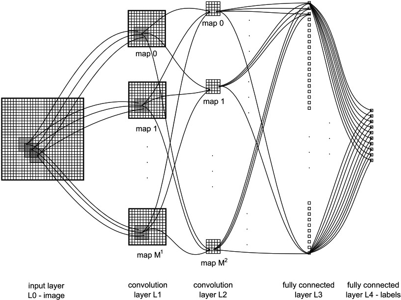$5\times 5$ and skipping factor of 1.

For the max-pooling layer, the length of the feature map is reduced in order to further minimize the number of model parameters. Consequently, the output of the max-pooling layer is based on the maximum activation over non-overlapping rectangular regions of size $(K_{x},K_{y})$ .

Finally, in the classification layer, the kernel sizes of the convolutional filters and max-pooling rectangles, as well as the skipping factors, are chosen. As a result, either the output maps of the last convolutional layer are down-sampled to 1 pixel per map or a fully connected layer combines the outputs of the top-most convolutional layer into a 1-D feature vector. In addition, one output unit of the top layer is associated with one specific class label.

Figure 2.

Conceptual representation of the Deep Learning-based Decision Tree Ensemble (DLDTE).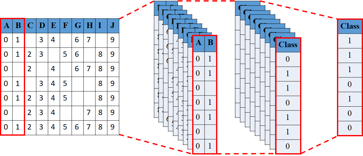

Figure 3.

An example of the sliding windows for 20% of 10 feature dimensions.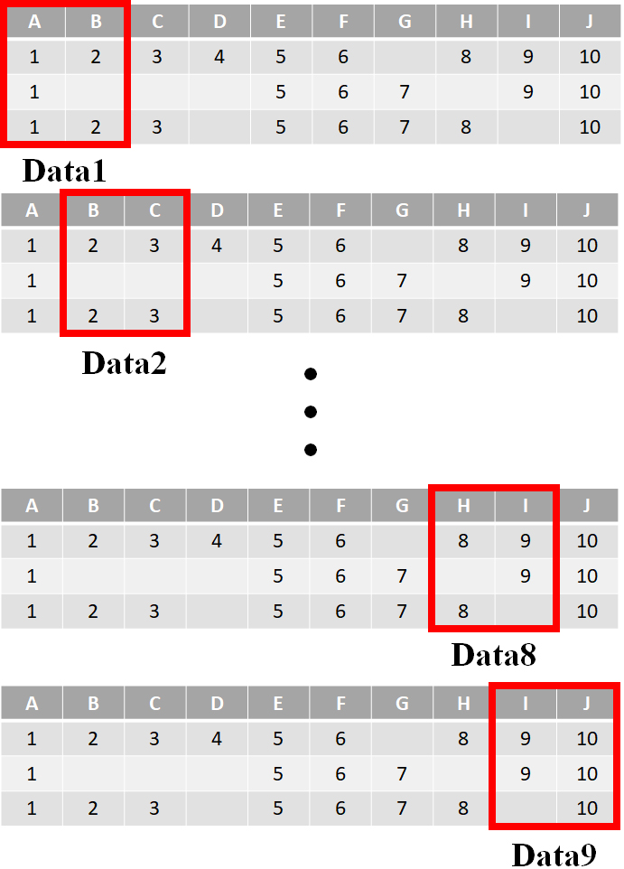

3. The proposed approach

Figure 2 shows a conceptual representation of the Deep Learning-based Decision Tree Ensemble (DLDTE), which is based on using the bounding box and sliding window strategies from the deep learning technique to divide a given incomplete dataset into a number of subsets for the construction of multiple decision trees. In particular, the proposed DLDTE approach is composed of several steps, described below.

First of all, the ‘window’ size parameter should be defined in the DLDET based on the feature dimensions of the incomplete dataset. In this study, the final classification performance for 20%, 40%, 60%, and 80% of the dataset dimensions is examined. For instance, if the collected dataset contains 50 feature dimensions for each data sample, then the window sizes for performance comparison are 10, 20, 30, and 40.

The ‘distance’ of the sliding window is another parameter that needs to be defined. Here, we fix it as one feature. The choice of the distance parameter will be described later. Figure 3 shows an example of the sliding windows for 20% of 10 feature dimensions. Each window size contains two dimensions and is based on the sliding distance, i.e. for one feature, there are nine sub-sets produced.

Next, the divided sub-sets are used to construct the corresponding decision tree models. For example, in Fig. 3, there are nine decision trees constructed. Finally, the given testing data point is fed into each of the decision tree ensembles according to the learned features. As a result, nine decision outputs are obtained with the final classification result obtained based on the voting method.

It should be noted that DLDTE is different from random forests as an ensemble of decision trees where each tree is trained by a random selection of a feature subset and the design of random forests algorithm is based on complete data. This means that missing value imputation should be performed for incomplete datasets before constructing random forests.

In this work, an initial study was conducted to decide the optimal distance. Two UCI datasets were chosen with 20% of the feature dimensions used as the window size and the window sizes of the sliding windows are set to 1, 3, 5, and 7 features. Figure 4 shows the final classification accuracies for different missing rates.

Figure 4.

The classification accuracies for different sliding window sizes over two datasets.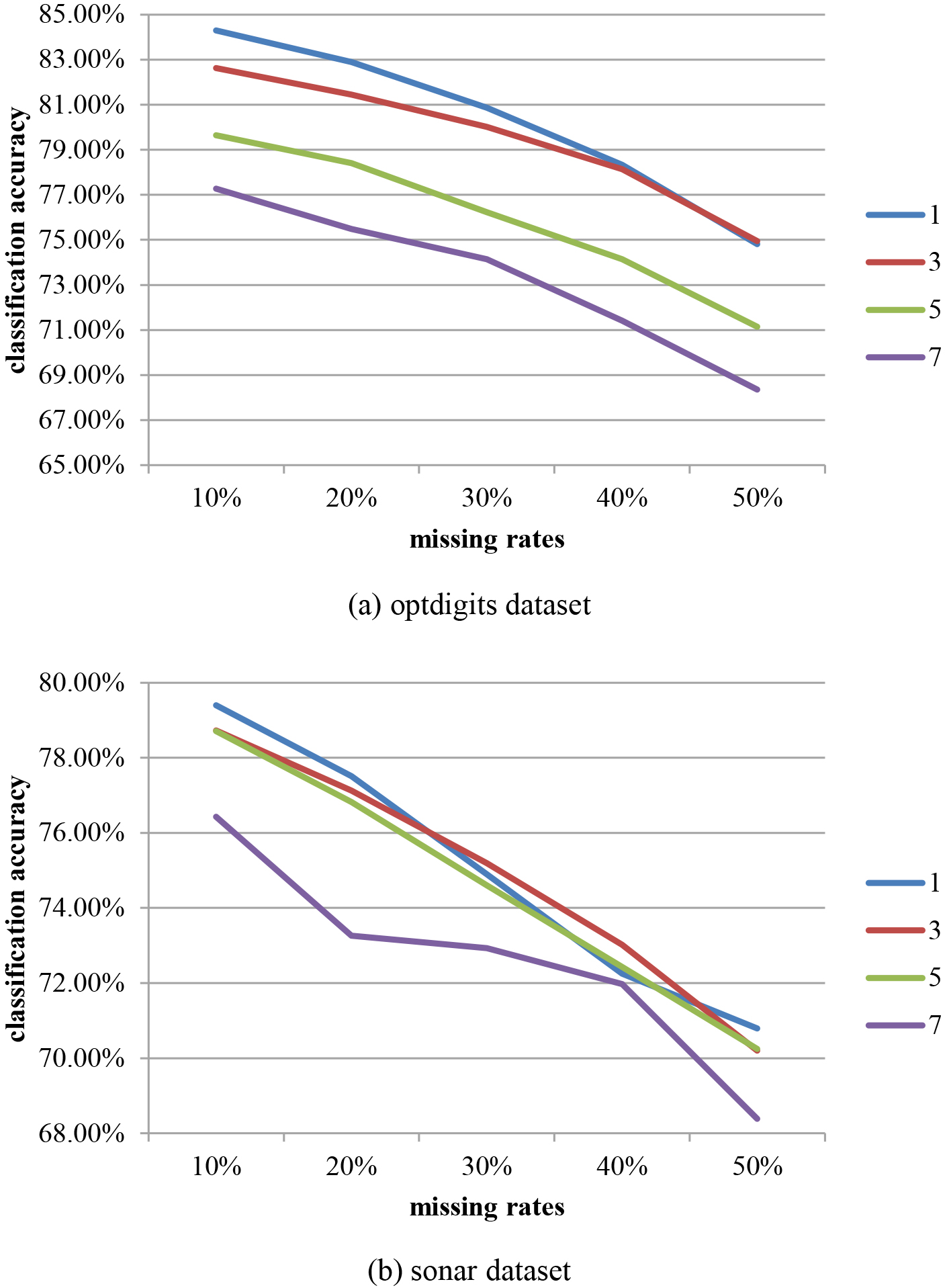

Regarding Fig. 4, there is degradation in the classification accuracy as the missing rates increase. Specifically, in most cases the best performance is obtained with a one feature sliding window. Therefore, this is the setting used in later experiments.

4. Experiments

4.1 Experimental setup

In this study, two medical domain problem datasets are chosen from the UCI Machine Learning Repository.1

¹
https://archive.ics.uci.edu/ml/index.php.
They contain different numbers of features, instances, and classes. The basic information about these datasets is shown in Table 1. In particular, the Gastroenterology dataset is about the prediction task for gastrointestinal lesions, whereas SCADI for the self-care problem of physical and motor disability.

Table 1
Basic information for the ten datasets

Dataset names No. of features No. of instances No. of classes

Gastroenterology 698 152 2

SCADI 205 69 6

There are two experiments discussed in this paper. The aim of the first experiment is to compare the classification performance of the proposed DLDTE approach and the baseline decision tree CART model.

Thus, each dataset is divided into 80% and 20% for the training and testing sets by 5-fold cross validation, respectively. In the training set, different missing rates (10%, 20%, 30%, 40%, and 50%) are simulated by the MCAR mechanism. Note that, since the distributions of the missing attributes should be different, each missing rate simulation is performed five times and the final performance is the average of the five different results.

Moreover, testing sets, with and without missing attributes, are also used to illustrate the classification performance of the different approaches. This is because, in practice, not only does the collected training set contain missing values, but the testing sets may also contain some missing values. Again, the simulation is carried out for the testing sets with missing values, using missing rates of 10%, 20%, 30%, 40%, and 50%.

The aim of the second experiment is to examine the classification performance of the proposed DLDTE approach in comparison with other missing value imputation methods. The settings for the training and testing sets and the missing rates are the same as in the first experiment. Of the baseline imputation methods, the mean/mode and k-nearest neighbor (KNN) methods are considered because they are widely used in related literatures, which can be regarded as the representative statistical and machine learning imputation methods, respectively [12, 31, 32, 33, 34].

The imputation process is performed on incomplete training and testing sets. After imputation of these incomplete sets, the CART decision tree method is used for the classification tasks to make possible a fair comparison with the direct handling methods used in this paper.
4.2 Results of study I

Dataset names	No. of features	No. of instances	No. of classes
Gastroenterology	698	152	2
SCADI	205	69	6

Tables 2–6 show the classification accuracies of the baseline and DLDET approach with different missing rates.

Table 2
Classification accuracies of the baseline and DLDTE for the 10% missing rate

	Baseline	DLDTE (window size)
		20%	40%	60%	80%
Gastroenterology	80.7%	68.08%	84.58%	84.30%	81.60%
SCADI	17.97%	28.40%	24.31%	22.23%	19.31%
Avg.	49.34% (4)	48.24% (5)	54.45% (1)	53.27% (2)	50.46% (3)

Table 3

Classification accuracies of the baseline and DLDTE for the 20% missing rate

	Baseline	DLDTE (window size)
		20%	40%	60%	80%
Gastroenterology	81.71%	66.67%	82.77%	83.25%	82.10%
SCADI	18.05%	28.00%	30.62%	30.79%	28.04%
Avg.	49.88% (4)	47.34% (5)	56.70% (2)	57.02% (1)	55.07% (3)

Table 4

Classification accuracies of the baseline and DLDTE for the 30% missing rate

	Baseline	DLDTE (window size)
		20%	40%	60%	80%
Gastroenterology	80.63%	68.98%	81.03%	81.18%	81.44%
SCADI	18.5%	25.92%	28.78%	26.08%	19.00%
Avg.	49.57% (4)	47.45% (5)	54.91% (1)	53.63% (2)	50.22% (3)

Table 5

Classification accuracies of the baseline and DLDTE for the 40% missing rate

	Baseline	DLDTE (window size)
		20%	40%	60%	80%
Gastroenterology	78.59%	68.18%	81.96%	80.84%	80.33%
SCADI	18.28%	21.94%	26.41%	30.41%	26.88%
Avg.	48.44% (4)	45.06% (5)	54.19% (2)	55.63% (1)	53.61% (3)

Table 6

Classification accuracies of the baseline and DLDTE for the 50% missing rate

	Baseline	DLDTE (window size)
		20%	40%	60%	80%
Gastroenterology	77.18%	63.15%	79.03%	78.10%	77.44%
SCADI	18.26%	25.34%	21.03%	20.63%	14.10%
Avg.	47.72% (4)	44.25% (5)	50.03% (1)	49.37% (2)	45.77% (3)

Results presented in Tables 2–6 indicate that the baseline method only performs better than DLDTE based on the 20% window size. In contrast, for most settings (i.e. 40%, 60%, and 80% window sizes), the proposed DLDTE approach outperforms the baseline method. On average, the best performance is obtained when the window size is set to 40% of the original dimensions.

Figure 5 shows the average classification accuracies obtained using the baseline and DLDTE methods over the two datasets. The proposed DLDTE approach significantly outperforms the baseline approach when using window sizes 40% and 60% of the original dimensions. The results show that the performance is similar to the baseline approach when the 80% window size is used because most of the original features are kept. The worst setting for the DLDTE approach is the 20% window size, which excludes many of the ‘good’ features from the subsets.

Figure 5.

Average classification accuracies of the baseline and DLDTE methods.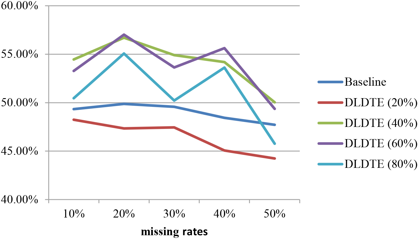

In addition, Fig. 6 shows the average classification accuracies of the baseline and DLDTE approaches over the two datasets for testing sets containing missing values. Comparison with Fig. 5, shows that when the testing sets contain some missing values, the classification performance is slightly lower than with the ones without missing values. Moreover, these results are similar to those seen in Fig. 5, indicating that the DLDTE method based on the 40% window size are more suitable for the two chosen medical domain problem datasets.

Figure 6.

Average classification accuracies of the baseline and DLDTE for testing sets with missing values.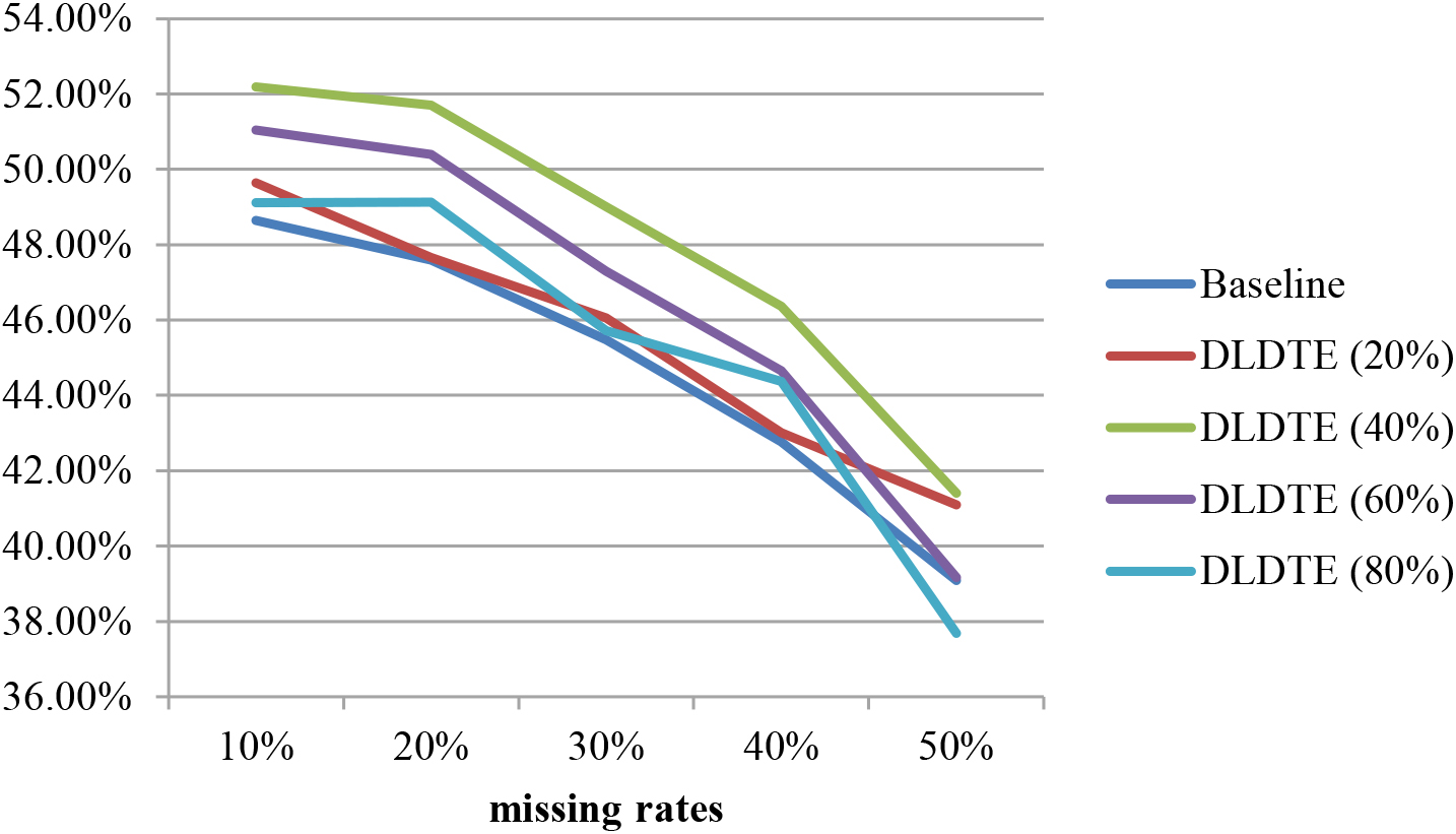

4.3 Results of study II

Tables 7–11 show the classification accuracies of the four baseline methods (including the case deletion, mean and KNN imputation methods, and CART) and DLDET obtained using different missing rates. Note that DLDET results are based on the 40% window size.

Table 7
Classification accuracies of the four baseline methods and DLDTE for the 10% missing rate

	Case deletion	Mean	CART	KNN	DLDTE
Gastroenterology	49.43%	80.38%	80.70%	80.93%	84.58%
SCADI	17.57%	19.04%	17.97%	17.72%	24.31%
Avg.	33.50% (5)	49.71% (2)	49.34% (3)	49.33% (4)	54.45% (1)

Table 8

Classification accuracies of the four baseline methods and DLDTE for the 20% missing rate

	Case deletion	Mean	CART	KNN	DLDTE
Gastroenterology	49.43%	81.71%	81.71%	83.98%	82.77%
SCADI	17.57%	18.05%	18.05%	18.97%	30.62%
Avg.	33.50 (5)	49.88% (3)	49.88% (3)	51.48% (2)	56.7% (1)

Table 9

Classification accuracies of the four baseline methods and DLDTE for the 30% missing rate

	Case deletion	Mean	CART	KNN	DLDTE
Gastroenterology	49.43%	80.04%	80.63%	80.18%	81.03%
SCADI	17.57%	19.51%	18.50%	17.27%	28.78%
Avg.	33.50% (5)	49.78% (2)	49.57% (3)	48.73% (4)	54.91% (1)

Table 10

Classification accuracies of the four baseline methods and DLDTE for the 40% missing rate

	Case deletion	Mean	CART	KNN	DLDTE
Gastroenterology	49.43%	74.68%	78.59%	79.95%	81.96%
SCADI	17.57%	17.43%	18.28%	19.11%	26.41%
Avg.	33.50% (5)	46.06% (4)	48.44% (3)	49.53% (2)	54.19% (1)

Table 11

Classification accuracies of the four baseline methods and DLDTE for the 50% missing rate

	Case deletion	Mean	CART	KNN	DLDTE
Gastroenterology	49.43%	80.40%	77.18%	78.42%	79.03%
SCADI	17.57%	16.25%	18.26%	18.19%	21.03%
Avg.	33.50% (5)	48.33% (2)	47.72% (4)	48.31% (3)	50.03% (1)

Similar to the results of Study I, it can be seen that the DLDTE approach is particularly suitable for the chosen medical datasets, and performs better than the four baseline approaches regardless of the missing rates considered.

In addition, Fig. 7 shows the average classification accuracies of the three baseline and DLDTE approaches obtained over the two medical datasets when the testing sets contain missing values. Note that the case deletion approach cannot be used in this case since any testing data with missing value(s) cannot be deleted. Again, these results show that DLDTE performs the best.

Figure 7.

Average classification accuracies of the four baseline and DLDTE approaches for testing sets with missing values.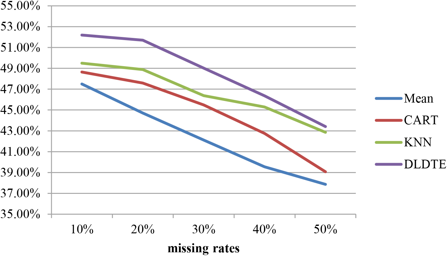

4.4 Discussion

Regarding the previous experimental results, the proposed DLDTE approach have been demonstrated its effectiveness for handling incomplete medical datasets containing missing values. That is, it can allow the classifier to provide higher rates of classification accuracy than other well-known missing value imputation methods. However, there are still some limitations of this study. First, the experimental datasets used in this paper are based on the numerical type of data. However, there are some other different types of data in medical domain datasets, which are the categorical type of data and the missed type of data containing both numerical and categorical types of data.

Second, since there are three kinds of missingness mechanisms, which are MCAR, MAR, and MNAR, the experiments are only based on the MCAR mechanism. Some incomplete medical datasets that contain missing values may not be occurred by random.

Third, it is usually the fact that many medical datasets whose feature dimensions are very high. An important data pre-processing step for effective data mining, i.e. feature selection, to filter out unrepresentative features is likely to improve the final classification performance. In this paper, feature selection is not executed to further examine the effect of feature selection on the missing value imputation performance.

5. Conclusion

Collected datasets with missing values make it problematic for many data mining and machine learning algorithms to successfully accomplish the data analysis task. One type of approach to solving the incomplete dataset problem is to construct specific models for missing value imputation, and another type of approach is to directly handle the incomplete datasets without considering missing value imputation, such as in the decision tree method.

The aim of this paper is to contribute to the second type of solution method, and introduce the novel Deep Learning-based Decision Tree Ensembles (DLDTE) approach. By borrowing the ideas of the bounding box and sliding window strategies used in the deep learning technique, a given incomplete dataset can be divided into incomplete subsets of fixed size by the bounding boxes or windows, and then each subset is trained to construct a decision tree model, resulting in decision tree ensembles for the given incomplete dataset.

In the experiments, two medical domain datasets containing different numbers of feature dimensions are used. The results show that the proposed DLDTE approach outperforms the baseline decision tree method for directly handling incomplete datasets, as well as two commonly used missing value imputation methods, mean and KNN, and the case deletion method for the missing rates of 10%, 20%, 30%, 40%, and 50%.

Regarding the limitations discussed in Section 4.4, several issues can be considered in the future. First, different types of missing data, including numerical, categorical and mixed data types, should be used to compare the performances of the proposed approach and related imputation methods. Second, other related medical datasets whose missing values were occurred by the MAR and MNAR mechanisms should also be examined in order to fully understand the performance of the proposed approach. Third, for high feature dimensional medical datasets, feature selection can be employed to analyze the importance of different features. Consequently, unrepresentative features are filtered out leading to new datasets with reduced feature dimensions. It would be worth investigating the effect of performing feature selection on the proposed approach and related missing value imputation methods. Fourth, to implement the proposed DLDTE approach in medical devices is another important issue to be investigated [35, 36, 37].

Footnotes

Conflict of interest

None to report.

Funding

The work was supported in part by the Ministry of Science and Technology of Taiwan (Grants MOST 105-2410-H-008-043-MY3 and MOST 111-2410-H182-015-MY3) and in part by Chang Gung Memorial Hospital at Linkou (Grants BMRPH13 and CMRPG3J0732).

References

van der Heijden

GJMG

Donders

ART

Stijnen

Moons

KGM

. Imputation of missing values is superior to complete case analysis and the missing-indicator method in multivariable diagnostic research: A clinical example. Journal of Clinical Epidemiology. 2006; 59: 1102-1109.

Troyanskaya

Cantor

Sherlock

Brown

Hastie

Tibshirani

Botstein

Altman

. Missing value estimation methods for DNA microarrays. Bioinformatics. 2001; 17: 520-525.

Stekhoven

Buhlmann

. Missforest-non-parametric missing value imputation for mixed-type data. Bioinformatics. 2012; 28: 112-118.

Liu

Chen

. Anomaly detection from incomplete data. ACM Transactions on Knowledge Discovery from Data. 2014; 9(2): article 11.

Liu

Musialski

Wonka

. Tensor completion for estimating missing values in visual data. IEEE Transactions on Pattern Analysis and Machine Intelligence. 2013; 35(1): 208-220.

Lakshminarayan

Harp

Samad

. Imputation of missing data in industrial databases. Applied Intelligence. 1999; 11(3): 259-275.

Song

Shepperd

Chen

Liu

. Can k-NN imputation improve the performance of C4.5 with small software project data sets? A comparative evaluation. Journal of Systems and Software. 2008; 81: 2361-2370.

Adhikari

Jiang

Zhan

Rawat

Aickelin

Khorshidi

. A comprehensive survey on imputation of missing data in internet of things. ACM Computing Surveys. 2022; 55(7): article no. 133.

Garcia-Laencina

Sancho-Gomez

J-L

Figueiras-Vidal

. Pattern classification with missing data: A review. Neural Computing & Applications. 2010; 19: 263-282.

10.

Olinsky

Chen

Harlow

. The comparative efficacy of imputation methods for missing data in structural equation modeling. European Journal of Operational Research. 2003; 151(1): 53-79.

11.

Batista

Monard

. An analysis of four missing data treatment methods for supervised learning. Applied Artificial Intelligence. 2003; 17: 519-533.

12.

Lin

W-C

Tsai

C-F

. Missing value imputation: A review and analysis of the literature (2006–2017). Artificial Intelligence Review. 2020; 53: 1487-1509.

13.

Tsikriktsis

. A review of techniques for treating missing data in OM survey research. Journal of Operations Management. 2005; 24: 53-62.

14.

Conroy

Eshelman

Potes

Xu-Wilson

. A dynamic ensemble approach to robust classification in the presence of missing data. Machine Learning. 2016; 102: 443-463.

15.

Liu

White

Thompson

Bramer

. Techniques for dealing with missing values in classification. Proceedings of the International Symposium on Advances in Intelligent Data Analysis, Reasoning about Data; 1997 Aug. 4–6; London UK; Springer; 1997. pp. 527-536.

16.

Krizhevsky

Sutskever

Hinton

. ImageNet classification with deep convolutional networks. Communications of the ACM. 2017; 60(6): 84-90.

17.

Schmidhuber

. Deep learning in neural networks: An overview. Neural Networks. 2015; 61: 85-117.

18.

Rubin

Little

RJA

. Statistical analysis with missing data, 2

{}^{\text{nd}}

Edition. New Jersey: Wiley; 2002.

19.

Heymans

Twisk

JWR

. Handling missing data in clinical research. Journal of Clinical Epidemiology. 2022; 151: 185-188.

20.

Chiu

C-C

Chan

S-Y

Wang

C-C

W-S

. Missing value imputation for microarray data: A comprehensive comparison study and a web tool. BMC Systems Biology. 2013; 7: S12.

21.

De Souto

MCP

Jaskowiak

Costa

. Impact of missing data imputation methods on gene expression clustering and classification. Bioinformatics. 2015; 16: 64-72.

22.

Luengo

Garcia

Herrera

. On the choice of the best imputation methods for missing values considering three groups of classification methods. Knowledge and Information Systems. 2012; 32: 77-108.

23.

Nishanth

Ravi

. Probabilistic neural network based categorical data imputation. Neurocomputing. 2016; 218: 17-25.

24.

Poulos

Valle

. Missing data imputation for supervised learning. Applied Artificial Intelligence. 2018; 32(2): 186-196.

25.

Ding

Simonoff

. An investigation of missing data methods for classification trees applied to binary response data. Journal of Machine Learning Research. 2010; 11: 131-170.

26.

Twala

. An empirical comparison of techniques for handling incomplete data using decision trees. Applied Artificial Intelligence. 2009; 23(5): 1-35.

27.

Twala

Jones

Hand

. Good methods for coping with missing data in decision trees. Pattern Recognition Letters. 2008; 29(7): 950-956.

28.

Goodfellow

Bengio

Couville

. Deep learning. Massachusetts: The MIT Press; 2016.

29.

leCun

Bengio

. Convolutional networks for images, speech, and time series. In: Arbib MA, editor. The handbook of brain theory and neural networks, 2

{}^{\text{nd}}

Edition. Massachusetts: The MIT Press; 1995. pp. 276-278.

30.

Ciresan

Meier

Masci

Gambardella

Schmidhuber

. Flexible, high performance convolutional neural networks for image classification. Proceedings of the International Joint Conference on Artificial Intelligence; 2011 July 16–22; Barcelona, Spain; AAAI Press; 2011. pp. 1237-1242.

31.

Marcelino

Leite

GMC

Celes

Pedreira

. Missing data analysis in regression. Applied Artificial Intelligence. 2022; 36(1). Available from: doi: 10.1080/08839514.2022.2032925.

32.

Luo

Qian

Wang

Guo

Sun

Lee

Teong

Lai

RTR

Miao

. Missing value imputation for diabetes prediction. Proceedings of the International Joint Conference on Neural Networks; 2022 July 18–23; Padua, Italy; IEEE; 2022. pp. 1-8.

33.

Shi

Wang

Yang

. An improved mean imputation clustering algorithm for incomplete data. Neural Processing Letters. 2022; 54: 3537-3550.

34.

Tsai

C-F

Y-H

. Empirical comparison of supervised learning techniques for missing value imputation. Knowledge and Information Systems. 2022; 64: 1047-1075.

35.

Badnjevic

Avdihodzic

Pokvic

. Artificial intelligence in medical devices: Past, present and future. Psychiatria Danubina. 2021; 33(3): S336-S341.

36.

Badnjevic

Pokvic

Deumic

Becirovic

. Post-market surveillance of medical devices: A review. Technology and Health Care. 2022; 30(6): 1315-1329.

37.

Gurbeta

Badnjevic

. Inspection process of medical devices in healthcare institutions: Software solution. Health and Technology. 2017; 7: 109-117.

Deep learning based decision tree ensembles for incomplete medical datasets

Abstract

BACKGROUND:

OBJECTIVE:

METHOD:

RESULTS:

CONCLUSION:

Keywords

1. Introduction

2. Literature review

2.1 Missing data mechanisms

2.2 Solutions to incomplete datasets

2.2.1 Missing value imputation

2.2.2 Direct handling methods

2.3 Deep learning

4.1 Experimental setup

Table 2 Classification accuracies of the baseline and DLDTE for the 10% missing rate

Table 7 Classification accuracies of the four baseline methods and DLDTE for the 10% missing rate

5. Conclusion

Footnotes

Conflict of interest

Funding

References

Table 2
Classification accuracies of the baseline and DLDTE for the 10% missing rate

Table 7
Classification accuracies of the four baseline methods and DLDTE for the 10% missing rate