Sage Journals: Discover world-class research

Abstract

A central problem in the context of the Web of Data as well as in data integration in general is to identify entities in different data sources that describe the same real-world object. There exists a large body of research on entity resolution. Interestingly, most of the existing research focuses on entity resolution on dense data, meaning data that does not contain too many missing values. This paper sets a different focus and explores learning expressive linkage rules from as well as applying these rules to sparse data, i.e. data exhibiting a large amount of missing values. Sparse data is a common challenge in application domains such as e-commerce, online hotel booking, or online recruiting. We propose and compare three entity resolution methods that employ genetic programming to learn expressive linkage rules from sparse data. First, we introduce the GenLinkGL algorithm which learns groups of matching rules and applies specific rules out of these groups depending on which values are missing from a pair of records. Next, we propose GenLinkSA, which employs selective aggregation operators within rules. These operators exclude misleading similarity scores (which result from missing values) from the aggregations, but on the other hand also penalize the uncertainty that results from missing values. Finally, we introduce GenLinkComb, an algorithm which combines the central ideas of the previous two into one integrated method. We evaluate all methods using six benchmark datasets: three of them are e-commerce product datasets, the other datasets describe restaurants, movies, and drugs. We show improvements of up to 16% F-measure compared to handwritten rules, on average 12% F-measure improvement compared to the original GenLink algorithm, 15% compared to EAGLE, 8% compared to FEBRL, and 5% compared to CoSum-P.

Keywords

Entity resolution sparse data linkage rules genetic programming link discovery

1. Introduction

As companies move to integrate data from even larger numbers of internal and external data sources and as more and more structured data is becoming available on the public Web, the problem of finding records in different data sources that describe the same real-world object is moving into the focus within even more application scenarios. There exists an extensive body of research on entity resolution in the Linked Data [30] as well as the database community [5,13]. However, most existing entity resolution approaches focus on dense data [6,19,31,32]. This paper sets an alternative focus and explores learning expressive linkage (matching) rules from as well as applying these rules to sparse data, i.e. data that contains a large amount of missing values.

Fig. 1.

Examples of attribute correspondences between product specifications: (left) specification from walmart.com, (center) centralised product catalog, and (right) specification from ebay.com.

A prominent example of an application domain that involves data exhibiting lots of missing values is e-commerce. Matching product data from different websites is difficult as most websites publish heterogeneous product descriptions using proprietary schemata which vary widely concerning their level of detail [29]. For instance in [38], we analyzed product data from 32 popular e-shops. The shops use within each product category (mobile phones, headphones, TVs) approximately 30 different attributes to describe items. The subset of the attributes that are used depends on the e-shop and even on the specific product. This leaves a data aggregator that collects product data for many e-shops into a rich schema with lots of missing values.

In [19], we presented GenLink, a supervised learning algorithm which employs genetic programming to learn expressive linkage rules from a set of existing reference links. These rules consist of attribute-specific preprocessing operations, attribute-specific comparisons, linear and non-linear aggregations, as well as specific weights and thresholds. The evaluation of GenLink has shown that the algorithm delivers good results with F-measures above 95% on different dense datasets such as sider-drugbank, LinkedMDB, and the restaurants dataset [19]. As shown in the evaluation section of this paper, GenLink as well as other entity resolution methods run into problems once the datasets to be matched are not dense, but contain larger amounts of missing values.

In order to overcome the challenge of missing values, this article introduces and evaluates three methods that build on the GenLink algorithm. First, we present GenLink Group Learning (GenLinkGL), an approach that groups linkage rules in order to cover different attribute combinations with specific rules. Next, we introduce the GenLink Selective Aggregations (GenLinkSA) algorithm which extends the original approach with selective aggregation operators to ignore and penalize comparisons that include missing values. Finally, we introduce GenLinkComb, an algorithm that combines the central ideas of the previous two into an integrated method. We evaluate all methods using six benchmark datasets: three of them are e-commerce product datasets, the other datasets describe restaurants, movies, and drugs.

The rest of this article is structured as follows: Section 2 formally introduces the problem of entity resolution. Section 3 gives an overview of the GenLink algorithm. Section 4 introduces the GenLinkGL, GenLinkSA, and GenLinkComb methods for dealing with sparse data. Section 5 presents the results of the experimental evaluation in which we compare the proposed methods with various baselines as well as other entity resolution systems. Section 6 discusses the related work.

Fig. 2.

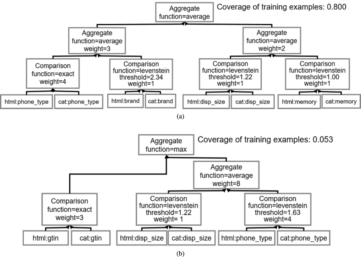
Example of two rules from the group for the phone category together with the coverage of each rule.

2. Problem statement

We consider two datasets, A the source, and B the target dataset. Each entity $e \in A \cup B$ consists of a set of attribute-value pairs (properties) $e = {(p_{1}, v_{1}), (p_{1}, v_{2}), \dots, (p_{n}, v_{n})}$ , where the attributes are numeric, categorical or free-text. For instance, an entity representing a product might be described by the name, GTIN number,1

¹
Global Trade Item Number (GTIN) is an identifier for trade items, developed by GS1. – www.gtin.info/.

color, camera properties as shown in Fig. 1. Our goal is to learn a matching rule that determines whether a pair of entities

(e_{a}, e_{b})

represents the same real-world object. Or formally [14], given the two datasets A and B, the objective is to find the set M consisting of all pairs of entities for which a relation

\sim_{R}

holds:

\begin{matrix} (1) & M = {(e_{a}, e_{b}); e_{a} \sim_{R} e_{b}, e_{a} \in A, e_{b} \in B} \end{matrix}

Additionally, we compute its complement set U defined as: $\begin{matrix} (2) & U = (A \times B) ∖ M \end{matrix}$

The purpose of relation $\sim_{R}$ is to relate all entities which represent the same real-world object [14].

To infer a rule specifying the conditions which must hold true for a pair of entities to be part of M, we rely on a set of positive correspondences $R_{+} \subseteq M$ that contains pairs of entities for which the $\sim_{R}$ relation is known to hold (i.e. which identify the same real world object). Analogously, we rely on negative correspondences $R_{-} \subseteq U$ that contain pairs of entities for which the $\sim_{R}$ relation is known not to hold (i.e. which identify different real world objects).

Given the correspondences, we can define the purpose of the learning algorithm as learning matching rules from a set of correspondences: $\begin{matrix} (3) & m : 2^{(A \times B)} \times 2^{(A \times B)} \to (A \times B \to [0, 1]) \end{matrix}$

The first argument in the above formula denotes a set of positive reference links, while the second argument denotes a set of negative reference links. The result of the learning algorithm is a linkage rule which should cover as many reference links as possible while generalising to unknown pairs.

3. Preliminaries

GenLink [19] is a supervised algorithm for learning expressive linkage rules for a given entity matching task. As all three algorithms that are introduced in this paper build on GenLink, this section summarises the main components of the GenLink algorithm. The full details of the algorithm are presented in [19].

3.1. Linkage rule format

GenLink represents linkage rules as a tree built out of four types of operators: (i) property operators, (ii) transformation operators, (iii) comparison operators and (iv) aggregation operators. The linkage rule tree is strongly typed i.e. only specific combinations of the four basic operators are allowed. Figure 2 shows two examples of linkage rules for matching data describing mobile phones. The formal grammar of the linkage rule format is found in [19].

Property operators Retrieves all values of a specific property p of each entity. For instance, in Fig. 2(a) the left most leaf in the tree retrieves the value for the “phone_type” property from the source dataset.

Transformation operators Transforms the values of a set of properties or transformation operators. Examples of common transformation functions include case normalization, tokenization, and concatenation of values from multiple operators.

Comparison operators GenLink offers three types of comparison operators. The first type of operators are character-based comparisons: equality, Levenshtein distance, and Jaro–Winkler distance. The second type includes token-based comparators: Jaccard similarity and Soft Jaccard similarity. The comparison is done over a single property or a specific combination of properties. The third type of comparison operators, numeric-similarity, calculate the similarity of two numbers. Examples of comparison operators can be seen in Fig. 2(a) as the parents of the leaf nodes.

Aggregation operators Aggregation operators combine the similarity scores from multiple comparison operators into a single similarity value. GenLink implements three aggregation operators. The maximum aggregation operator aggregates similarity scores by choosing the maximum score. The minimum aggregation operator chooses the minimum from the similarity score. Finally, the average aggregation operator combines similarity scores by calculating their weighted average.

Note that these aggregation functions can be nested, meaning that non-linear hierarchies can be learned. For instance, in Fig. 2(a), four different properties are being compared (“phone_type”, “brand”, “memory” and “display_size”). Subsequently, two average aggregations are applied to aggregate scores from phone_type and brand, and memory and display_size, respectively. Finally, a third average aggregation is applied to aggregate scores from the previous aggregators.

Compared to other linkage rule formats, GenLink’s rule format is rather expressive, as it is subsuming threshold-based boolean classifiers and linear classifiers, hence allows for representing non-linear rules and may include data transformations which normalize the values prior to comparison [19]. Therefore, it allows rules to closely adjust to the requirements of a specific matching situation by choosing a subset of the properties of the records for the comparison, normalizing the values of these properties using chains of transformation operators, choosing property-specific similarity functions, property-specific similarity thresholds, assigning different weights to different properties, and combining similarity scores using hierarchies of aggregation operators.

3.2. The GenLink algorithm

The GenLink algorithm learns a linkage given a set of positive and negative training examples. The GenLink algorithm starts with an initial population of candidate solutions which is evolved iteratively by applying a set of genetic operators.

Generating initial population The algorithm finds a set of property pairs which hold similar values before the population is generated. Based on that, random linkage rules are built by selecting property pairs from the set and building a tree by combining random comparisons and aggregations.

Selection The population of linkage rules is bred and the quality of the linkage rules is assessed by a fitness function using the training data. The purpose of the fitness function is to assign a value to each linkage rule which indicates how close the given linkage rule is to the desired solution. The algorithm uses Matthews Correlation Coefficient (MCC) as fitness measure. MCC [25] is defined as the degree of the correlation between the actual and predicted classes or formally: $\begin{array}{l} MCC \\ (4) & = \frac{t p \times t n - f p \times f n}{\sqrt{(t p + f p) (t p + f n) (t n + f p) (t n + f n)}} \end{array}$

The training data consists of a set of positive correspondences (linking entities identifying the same real-world object) and a set of negative correspondences (stating that entities identify different objects). The predictions of the linkage rule is compared with the positive correspondences, counting true positives and false negatives, the negative correspondences, counting false positives and true negatives. In order to prevent linkage rules from growing too large and potentially overfit the training data, we penalize linkage rules depending on the number of operators the rules contain: $\begin{matrix} (5) & fitness = MCC - 0.05 \times operatorcount \end{matrix}$

Once the fitness is calculated for the entire population, GenLink selects individuals for reproduction by employing the tournament selection method.

Crossover GenLink applies six types of crossover operators:

Function crossover. The function crossover selects one comparison operator at random in each linkage rule and interchanges the similarity functions between the selected operators.

Operators crossover. The operators crossover is designed to combine aggregation operators from two linkage rules, by selecting an aggregation from each linkage rule and combining their respective comparisons. The crossover selects all comparisons from both aggregations and removes each comparison with a probability of 50%.

Aggregator crossover. In order to learn aggregation hierarchies, the aggregation crossover operator selects a random aggregation or comparison operator in the first linkage rule and replaces it with a random aggregation or comparison operator from the second linkage rule.

Transformation crossover. This crossover builds chains of transformations. To recombine the transformations of two linkage rules the transformation operators of both rules are combined by randomly selecting an upper and a lower transformation operator, recombining their paths via a two point crossover and removing duplicated transformations.

Threshold crossover and Weight crossover. The last two types of crossovers are used to recombine thresholds and weights respectively, for a random comparison operator in each linkage rules, by averaging their thresholds/weights.

An in-depth discussion of the crossover operators is provided in [19].

4. Approaches

In [37] we have shown that the GenLink algorithm struggles to optimise attribute selection for sparse datasets. On an e-commerce dataset containing many low-density attributes the algorithm only reached a F-measure of less than 80%, in contrast to the above 95% results that are often reached on dense datasets. In the following, we propose three algorithms that build on the GenLink algorithm and enable it to properly exploit sparse attributes for matching decisions. The GenLinkGL algorithm learns a group of matching rules for the given matching task (group generation) and applies different rules from within the group to discover correspondences at runtime (group application). Next we introduce selective aggregations, new operators within the GenLink algorithm that can better deal with missing values. Finally, we introduce GenLinkComb approach which combines the central ideas of the previous two approaches into a single method.

4.1. The GenLinkGL algorithm

The GenLink algorithm lacks the capability to optimise attribute selection when dealing with sparse data. The algorithm will select a combination of dense attributes while sparse attributes will rarely be selected. This behavior influences adversely cases in which values from relatively dense attributes are missing. For instance, when matching product data describing mobile phones from different e-shops, the brand, phone type, and memory properties will be rather important for the matching decisions and these attributes will also likely be rather dense as they are provided by many e-shops. Therefore, GenLink will focus on these attributes and due to the penalty on large rules (compare Equation (5)) will not include alternative attribute combinations involving low-density properties, such as gtin, display size, or operating system. In cases in which a value of one of these dense attributes is missing, the algorithm will likely fail to discover the correct match, while by exploiting a combination of alternative low-density attributes it would have been possible to recognize that the both records describe the same product. Including all alternative attribute combinations into a single linkage rule would result in rather large rules containing multiple alternative branches that encode the different attribute combinations. Due to the penalty for large rules from Equation (5), only the most important alternative attribute combinations will be included into the rules, whereas combinations having a lower coverage will be left unused.

A way to deal with this problem could be to loosen the size penalty in Equation (5), however removing (or loosening) the penalty has the potential to result in an overfitted model. With GenLink Group Learning (GenLinkGL), we choose an alternative approach – instead of trying to grow very large rules that cover different attribute combinations, we learn sets of rules in which each rule is optimized for a specific attribute combination. The method allows us to separate more clearly the issue of avoiding overfitting rules while still being able to cover multiple attribute combinations. By combining multiple combinations of properties in a group, the learning algorithm is given the freedom to optimize matching rules not only for the most common attribute combinations, but also for less common combinations involving sparse properties, as a result increasing the overall recall. In the following, we describe how GenLinkGL combines rules into groups and later selects a rule from the group in order to match a pair of records having a specific property combination.

Algorithm 1

Generating a group of linkage rules

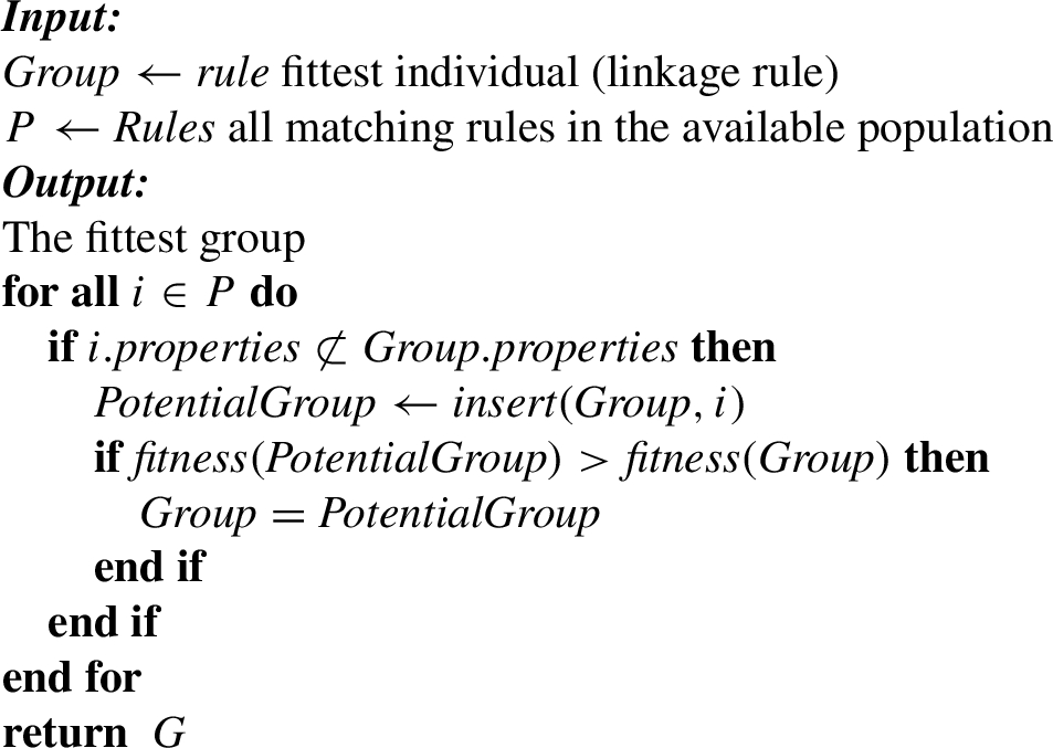
Group generation The basic idea of the first algorithm, presented in Algorithm 1, is that by grouping different linkage rules using different properties we could circumvent the missing values in the data. The initial group is populated with the fittest individual from the population generated by GenLink. Subsequently, an initial fitness for this group is computed using the MCC (compare Equation (4)).

Motivated by the GenLink algorithm, our algorithm builds a group that maximises fitness. To do this at each learning iteration, the algorithm iterates through the entire population of linkage rules and combines their individual fitness. We restrict the combination to linkage rules whose properties are not a subset of the properties of the group and include a linkage rule that has at least one new property that is not present in the group. We combine the fitness of the linkage rules by summing the number of correctly predicted instances in the training set (compare Equations (6) and (7)), calculating for each individual the percentage of the coverage of training examples in the group. Once the correctly predicted instances are summed the current fitness function is applied to the group. If the fitness of that combination is greater than the current fittest group, the new group becomes the best group. As an output the algorithm gives the fittest group. $\begin{array}{l} (6) & \begin{matrix} t p_{group} & = \sum_{i = 1}^{| G |} distinct t p_{i} \\ f p_{group} & = | R_{+} | - t p_{group} \end{matrix} \\ (7) & \begin{matrix} t n_{group} & = \sum_{i = 1}^{| G |} distinct t n_{i} \\ f n_{group} & = | R_{-} | - t n_{group} \end{matrix} \end{array}$

Algorithm 1 can potentially lead to groups containing a large number of rules, up to the complete population of learned rules. In this case, the algorithm is prone to overfitting, since the population might capture the entire training set. In order to prevent this, we penalize groups containing a large number of rules: ${fitness}_{group} = {MCC}_{group} - c \times rulecount$ . Where $c = (0.001, 0.003, 0.005)$ is a small constant which is set depending on the number of rules in the population. The larger the population, the bigger the chance for overfitting. Therefore, the constant should be higher for larger populations in order to penalise the fitness more. By penalizing the fitness by the number of members in the group, we ensure that there will be no unneeded bloating of the learned group.

For example, let the linkage rule in Fig. 2(a) be the fittest individual after the nth learning iteration of the algorithm. The initial group contains this linkage rule. The group would not be able to correctly predict correspondences that can only be found using a combination of the gtin, phone_type and memory properties. In the first iteration, we combine the group with the linkage rule in Fig. 2(b) which exploits the gtin property in cases in which this property is filled (coverage of training examples 0.053). As a result, the correspondences above are generated by the group leading to better fitness.

Algorithm 2

Applying a group of rules to match pairs of sparse records

Group application We use Algorithm 2 to apply a group of matching rules generated by Algorithm 1 to match pairs of sparse records. The individuals in the input group are sorted by the percentage of coverage. Sorting enables Algorithm 2 to find the more influential individual rules in less iterations. For each pair the algorithm iterates through the group of matching rules. If the pair to be matched contains the same properties as in the matching rule, the matching rule is applied. If there is no matching rule which has the exact properties as the instances, the top matching rule is applied. For instance, when matching (a) the specification from walmart.com with the product catalog and (b) the specification from ebay.com with the product catalog from Fig. 1, the algorithm would use the first rule from Fig. 2 for the a pair, but use the second matching rule from Fig. 2 for the b pair since in b one of the specifications does not have a value for the display_size attribute, however it contains a gtin attribute.

4.2. The GenLinkSA algorithm

An alternative to learning groups of linkage rules specializing on a specific attribute combination each is to learn larger rules covering more attributes and apply a penalty for the uncertainty that arises from values missing in these attributes. For instance, a larger rule could rely on five properties for deciding whether two records match. If two of the five properties have missing values, the remaining three properties can still be used for the matching decision. Nevertheless, a decision based on three properties should be considered less certain than a decision based on five properties. In order to compensate for this uncertainty, we can require the values of the remaining three properties to be more similar than the values of the five properties in the original case in order to decide for a match. The GenLink Selective Aggregations (GenLinkSA) algorithm implements this idea by changing the behavior of the comparison operators as well as the aggregation operators in the original GenLink algorithm.

Fig. 3.

GenLinkSA rule for the phone category.

NULL-enabled comparison operators The original GenLink algorithm does not distinguish between a pair of different values and a pair of values containing a missing value. In both cases, the algorithm assigns the similarity score 0. This is problematic when similarity scores from multiple comparison operators are combined using the aggregation function average or minimum, as the resulting similarity score will be unnaturally low for the case of record pairs containing missing values. In order to deal with this problem, GenLinkSA amends the comparison operators with the possibility to return the value NULL: a GenLinkSA comparison operator will return NULL if one or both values are missing. If both values are filled, the operator will apply its normal similarity function and return a value in the range $[0, \dots, 1]$ .

Selective aggregation operators The GenLink aggregation operators calculate a single similarity score from the similarity values of multiple comparison operators using an aggregation function such as weighted average, minimum, or maximum. GenLinkSA adjusts the aggregation operators to apply the aggregation function only to non-NULL values. In order to compensate the uncertainty that results from missing values (comparison operators returning the value NULL), the similarity score that results from the aggregation is reduced by constant factor α for each comparison operators that returns a NULL value. Thus, all non-NULL similarity scores are aggregated and a penalty is applied for each property pair containing missing values. Formally, a GenLink aggregation is defined by the following: $\begin{matrix} (8) & \begin{matrix} S^{a} : (S^{*} \times N^{*} \times F^{a}) \to S \\ (\bar{s}, \bar{w}, f^{a}) \to ((e_{a}, e_{b}) \to f^{a} (s_{e}, w)) \end{matrix} \end{matrix}$ with $s_{e} : (s_{1} (e_{a}, e_{b}), s_{2} (e_{a}, e_{b}), \dots, s_{n} (e_{a}, e_{b}))$

The first argument $S^{*}$ contains the similarity scores returned by the operators of this aggregation while the second argument $N^{*}$ contains a weight for each of the operators, finally the third argument $F^{a}$ represents the aggregation function that is applied to compute the similarity score S.

Given the aggregation operators, we can now define GenLinkSA’s selective aggregation operators as: $\begin{matrix} (9) & \begin{matrix} S^{a} : (S^{*} \times N^{*} \times F^{a}) \to S \\ (\bar{s}, \bar{w}, f^{a}) \to ((e_{a}, e_{b}) \to f^{a} (s_{e}, w)) - υ \end{matrix} \end{matrix}$ with $s_{e} : (s_{1} (e_{a}, e_{b}), s_{2} (e_{a}, e_{b}), \dots, s_{n} (e_{a}, e_{b})) υ = β \times | {s_{i} (e_{a}, e_{b}); s_{i} (e_{a}, e_{b}) \to null \land s_{i} \in s_{e}} |$

Where the uncertainty factor υ is defined as the number of NULL values multiplied by a small valued constant factor $β = (0.01, 0.03, 0.05)$ . The uncertainty factor serves to penalize the rule for each NULL similarity operator. As the overall similarity score is reduced by the uncertainty factor, the values of the non-NULL properties must be more similar in order to reach the same similarity score as for a pair in which all properties are filled.

For example, let the rule learned by the GenLinkSA algorithm be the one shown in Fig. 3 and let instances for matching be (a) the specification from walmart.com that should be matched with the product catalog and (b) the specification from ebay.com to be matched with the product catalog from Fig. 1. When matching (a) only a small penalty will be applied since for five out of six comparisons a non-NULL similarity score will be returned and only the comparison for one property (comp_os) will be penalised. On the other hand, the pair (b) will be heavily penalised since four of the six comparisons will return NULL values. Evidently, this method will discourage high similarity scores in the presence of missing values and will thus refrain from considering borderline cases with missing values as matches, resulting in a higher precision.

4.3. The GenLinkComb algorithm

GenLinkGL and GenLinkSA tackle the issue of missing values differently. Namely, GenLinkGL strives to group matching rules exploiting different combinations of attributes and thus is able to apply alternative rules given that values of important attributes are missing. By being able to exploit alternative property combinations, GenLinkGL is tailored to improve recall. On the other hand, by penalizing comparisons with missing values, GenLinkSA incentivises learning matching rules that include more properties and substantially lowers the similarity scores of uncertain pairs, and by that improves precision. As the basic ideas behind GenLinkGL and GenLinkSA do not exclude each other but are complementary, a combination of both methods into a single integrated method could combine their advantages: optimize rules for alternative attribute combinations while at the same time dealing with the uncertainty that arises from missing values inside the rules. The GenLinkComb algorithm achieves this by combining the GenLinkSA and the GenLinkGL algorithms as follows: GenLinkComb uses the GenLinkSA algorithm to evolve the population of linkage rules. In each iteration of the learning process, GenLinkComb groups the learned rules together using the GenLinkGL algorithm. By being able to deal with missing values either inside the rules using the selective aggregation operators or within the grouping of rules, the GenLinkComb learning algorithm has a higher degree of freedom in searching for a good solution.

5. Evaluation

We use six benchmark datasets to evaluate the proposed methods: three e-commerce product datasets, and three datasets describing restaurants, movies, and drugs. In addition to comparing GenLinkGL, GenLinkSA, and GenLinkComb with each other, we also compare the approaches to existing systems including CoSum-P, FEBRL, EAGLE, COSY, MARLIN, ObjectCoref, and RiMOM. The following sections describe the six benchmark datasets, give details about the experimental setup, and present and discuss the results of the matching experiments.

Table 1
Property densities in the Abt–Buy and Amazon–Google datasets

Dataset Property Density (A/B)%

Abt–Buy Original Attributes

Product Name 100

Description 63

Manufacturer 48

Price 36

Extracted Attributes

Model 91

Brand 72

Amazon–Google Original Attributes

Product Name 100

Description 70

Manufacturer 52

Price 31

Extracted Attributes

Model 88

Brand 76

Dataset	Property	Density (A/B)%
Abt–Buy	Original Attributes
Product Name	100
Description	63
Manufacturer	48
Price	36
Extracted Attributes
Model	91
Brand	72
Amazon–Google	Original Attributes
Product Name	100
Description	70
Manufacturer	52
Price	31
Extracted Attributes
Model	88
Brand	76

5.1. Datasets

Product matching datasets We use three different product datasets for the evaluation:

Abt–Buy dataset:

The dataset includes correspondences between 1081 products from Abt.com and 1092 from Buy.com. The full input mapping contains 1.2 million correspondences, from which 1000 are annotated as positive correspondences (matches). Each product is described by up to four properties: product name, description, manufacturer, and price. The dataset was introduced in [21]. Since the content of the product name property is a short text listing various product features rather than the actual name of the product, we extract the product properties Brand and Model from the product name values using the dictionary-based method presented in [39]. Table 1 shows the densities of the original as well as the extracted properties. We choose the Abt–Buy dataset because it is widely used to evaluate different matching systems [4,8].

Amazon–Google dataset:

The dataset [21] includes correspondences between 1363 products from Amazon and 103,226 from Google. The full input mapping contains 4.4 million correspondences, from which 1000 are annotated as matches. Each entity of the dataset contains the same properties as the Abt–Buy dataset. We also extract Brand and Model values from the product names using the same method as for the Abt–Buy dataset. The Amazon–Google data set has also been widely used as benchmark data set [21].

WDC Product Matching Gold Standard:

This gold standard [38] for product matching contains correspondences between 1500 products (500 each from the categories headphones, mobile phones, and TVs), collected from 32 different websites and a unified product catalog containing 150 products with the following distribution: (1) Headphones – 50, (2) Phones – 50, and (3) TVs – 50. The data in the catalog has been scraped from leading shopping services, like Google Shopping, or directly from the vendor’s website. The gold standard contains 500 positive correspondences (matches) and more than 25000 negative correspondences (non-matches) per category. Compared to the Amazon–Google and Abt–Buy datasets, the WDC Product Matching Gold Standard is more heterogeneous as the data has been collected from different websites. The gold standard also features a richer schema containing over 30 different properties for each product category.

Table 2
Properties and property density of the WDC product matching gold standard, restaurants, sider-drugbank and LinkedMDB datasets. Note that properties having a density below 10% are not included into the table

Dataset Property Density (A/B) %

WDC Gold Standard Headphones

Brand 97/100

Item Type 87/100

MPN 60/86

Color 56/96

Sensitivity 53/88

Impedance 53/92

Cup Type 47/38

Form Factor 43/77

Magnet Mat. 27/51

Diaphragm 25/35

Phones

Phone Type 91/100

Memory 87/95

Brand 86/100

Color 79/43

Display Size 71/92

Rear Cam. Res. 70/85

OS 64/64

Display Res. 48/53

Processor 28/36

Front Cam. Res. 20/66

TVs

Brand 100/100

Item Type 91/100

Display Type 81/85

Display Size 65/96

Display Res 55/87

Tot. Size 51/74

Ref. Rate 50/96

Img. Asp. Rat. 38/60

Connectivity 35/61

Resp. Time 10/25

Restaurant Name 100

Address 100

Contact 100

Type 100

Sider-Drugbank Name 100/100

Indication 100/93

LinkedMDB Name 100/100

Director 100/100

Rel Date 100/100

Studio 95/97

Dataset	Property	Density (A/B) %
WDC Gold Standard	Headphones
Brand	97/100
Item Type	87/100
MPN	60/86
Color	56/96
Sensitivity	53/88
Impedance	53/92
Cup Type	47/38
Form Factor	43/77
Magnet Mat.	27/51
Diaphragm	25/35
Phones
Phone Type	91/100
Memory	87/95
Brand	86/100
Color	79/43
Display Size	71/92
Rear Cam. Res.	70/85
OS	64/64
Display Res.	48/53
Processor	28/36
Front Cam. Res.	20/66
TVs
Brand	100/100
Item Type	91/100
Display Type	81/85
Display Size	65/96
Display Res	55/87
Tot. Size	51/74
Ref. Rate	50/96
Img. Asp. Rat.	38/60
Connectivity	35/61
Resp. Time	10/25
Restaurant	Name	100
Address	100
Contact	100
Type	100
Sider-Drugbank	Name	100/100
Indication	100/93
LinkedMDB	Name	100/100
Director	100/100
Rel Date	100/100
Studio	95/97

Other entity resolution datasets In order to be able to compare our approaches to more reference systems, as well as to showcase the ability of our algorithms to perform on datasets from different application domains, we also run experiments with the three benchmark datasets that were used in [19]:

Restaurant dataset:

The dataset contains correspondences between 864 restaurant entities from the Fodor’s and Zagat’s restaurant guides. Specifically, 112 duplicate records were identified.

Sider-Drugbank dataset:

The dataset contains correspondences between 924 drug entities in the Sider dataset and 4772 drug entities in the Drugbank dataset. Specifically, there have been 859 duplicate records identified.

LinkedMDB dataset

This dataset contains 100 correspondences between 373 movies. The authors note that special care was taken to include relevant corner cases such as movies which share the same title but have been produced in different years.

Tables 1 and 2 give an overview of densities of properties in the six evaluation datasets. If the density of a property differs in the source (A) and the target (B) dataset, both densities are reported. For the Abt–Buy and Amazon–Google datasets, we show all original property densities as well as the density of the extracted properties. The Abt–Buy and Amazon–Google datasets follow a similar distribution in which only the product name property has a density of 100%. It is worth to note that the product name property in these datasets is actually a short description of the product mentioning different properties rather than the actual product name. WDC Product Matching Gold Standard contains a small set of properties with a density above 90% while most properties belong to the long tail of rather sparse properties [38].

5.2. Experimental setup

Baselines As baselines for the WDC gold standard, we repeat the TF-IDF cosine similarity and Paragrph2Vec experiments presented in [38]. Additionally, we learn decision trees and random forests. The first baseline, considers pair-wise cosine matching of product descriptions for which TF-IDF vectors are calculated using the bag-of-words feature extraction method. The second baseline, employs the distributed bag-of-words method to calculate Paragraph2Vec embeddings [23] for product names using 50 latent features. The embeddings are compared using cosine similarity. Decision trees and random forests are learned in Rapidminer2

²
https://rapidminer.com/

using grid search parameter optimization as well as offering the learning algorithm different similarity metrics (e.g. Jaccard, Jaro–Winkler, numeric).

Other entity resolution systems In order to set the GenLink results into context, we also ran the WDC gold standard experiments with EAGLE [34], a supervised matching system that also employs genetic programming,3

http://aksw.org/Projects/LIMES.html

FEBRL [8]4

⁴

https://sourceforge.net/projects/febrl/

an entity resolution system that internally employs a support vector machine, and CoSum-P [44], an unsupervised system that treats entity resolution as a graph summarization problem. We pre-compute attribute similarities for CoSum-P as described in [44].

Fig. 4.

Handwritten matching rule for the headphones category.

Additionally, we provide a comparison to handwritten Silk rules. These rules are composed of up to six properties for each product category and were written by the authors of this article using their knowledge about the respective domains as well as statistics about the datasets. As an example, the handwritten rule that was used for matching headphones, shown in Fig. 4, implements the intuition that if the very sparse properties html:gtin or html:mpn match exactly, the record pair should be considered as a match. If these numbers are not present or do not match, the rule should fall back to averaging the similarity of the properties html:model, html:impedence and html:headphone_cup_type giving most weight to html:model.

Table 3

Available aggregation, comparison, and transformation functions. The transformation functions are used only for non-product datasets

Comparison	Aggregation	Transformations
Exact Similarity	Average	Tokenize
Levenstein Distance	Maximum	Lower Case
Jaccard Similarity	Minimum	Concatenate
Number Similarity

GenLinkGL, GenLinkSA, and GenLinkComb The GenLinkGL, GenlinkSA, and GenLinkComb algorithms were implemented on top of the Silk Framework.5

⁵

http://www.silkframework.org

The source code of the original GenLink implementation6

⁶

https://github.com/silk-framework/silk To be noted that the 2.6.0 version was used for the experiments.

as well as the source code of GenLinkGL, GenlinkSA, GenLinkComb algorithms7

⁷

https://github.com/petrovskip/silk.2.6-GenLinkSA and https://github.com/petrovskip/silk.2.6-GenLinkGL.

are publicly available, so all results presented in this article can be replicated. Table 3 gives an overview of the aggregation, comparison, and transformation functions the algorithms could choose from in the experiments. It should be noted that for each aggregation operator there exists a corresponding selective aggregation operator. Hyperparameters are set using grid search. Even though grid search was run for each dataset, the resulting parameter values were the same for all datasets. Table 4 summarises the parameters that were used for GenLink and its variants in the experiments. All experiments are run 10 times and the results are averaged.

Table 4

GenLink (GL/SA/Comb) parameters

Parameter	Value
Population size $\| P \|$	1000
Maximum iterations I	100
Selection method	Tournament selection
Tournament size	10
Probability of Crossover	50%
Probability of Mutation	50%
Stop Condition	F-measure = 1.0
Matching Rule Penalty c	0.03
Uncertainty constant β	0.05

GenLink and its variants as well as EAGLE were trained on a balanced dataset consisting of 66% of the positive correspondences and the same number negative correspondences. The systems were tested afterwards using the remaining 33% of the correspondences. For training FEBRL, we calculated TF-IDF scores and cosine similarity for all pairs given in the dataset. As with GenLink and EAGLE, FEBRL was trained on 66% of the data and evaluated on the rest. For the experiments on the Abt–Buy and Amazon–Google datasets, all systems were trained using the original as well as the extracted attribute-value pairs.

Preprocessing The restaurants, movies, and drugs datasets have an original density of over 90%. In order to use them to evaluate how the different approaches perform on sparse data, we systematically removed 25%, 50% and 75% of the values. More precisely, we first randomly sample 50% of properties (not including the name property) and for those we randomly select 25%, 50% and 75% of the values and removed the rest, thus introducing greater percentage of null values in the datasets. We do not remove values from all properties since we want to create a similar sparseness distribution as we found in the product datasets. We do not remove the name property since it is the only reliable identifier for a human, i.e without it even a human cannot decide whether two entities are the same.

5.3. Product matching results

Table 5 gives an overview of the matching results on the WDC gold standard. Moreover, we compare results of: (i) the baselines, (ii) handwritten matching rules, (iii) the GenLink algorithm, (iv) GenLinkGL, (v) GenLinkSA, and (vi) GenLinkComb. In addition, we compare to the GenLink results with three state-of-the-art matching systems: (i) EAGLE [34], (ii) FEBRL [21], and (iii) CoSum-P [44].

Table 5
Matching results per category for the WDC product matching gold standard

Precision Recall F-measure

Headphones

Baseline TF-IDF Cosine 0.622 0.559 0.588

Baseline Pargraph2vec 0.667 0.685 0.675

Baseline Decision Tree 0.892 0.712 0.791

Baseline Random Forest 0.891 0.764 0.822

Handwritten Rule 0.841 0.838 0.839

EAGLE [34] 0.661 0.905 0.763

GenLink [19] 0.692 0.946 0.799

CoSum-P [44] 0.795 0.868 0.830

FEBRL [8] 0.884 0.837 0.850

GenLinkGL 0.837 0.924 0.888

GenLinkSA 0.922 0.925 0.923

GenLinkComb 0.920 0.961 0.940

Phones

Baseline TF-IDF Cosine 0.385 0.676 0.491

Baseline Pargraph2vec 0.497 0.624 0.553

Baseline Decision Tree 0.751 0.600 0.667

Baseline Random Forest 0.771 0.726 0.747

Handwritten Rule 0.656 0.722 0.687

EAGLE [34] 0.699 0.672 0.685

GenLink [19] 0.708 0.715 0.712

CoSum-P [44] 0.746 0.821 0.781

FEBRL [8] 0.792 0.748 0.776

GenLinkGL 0.742 0.894 0.808

GenLinkSA 0.813 0.737 0.773

GenLinkComb 0.815 0.886 0.849

TVs

Baseline TF-IDF Cosine 0.661 0.474 0.554

Baseline Pargraph2vec 0.654 0.553 0.572

Baseline Decision Tree 0.839 0.714 0.771

Baseline Random Forest 0.785 0.810 0.797

Handwritten Rule 0.782 0.716 0.747

EAGLE [34] 0.722 0.674 0.697

GenLink [19] 0.790 0.711 0.748

CoSum-P [44] 0.779 0.814 0.796

FEBRL [8] 0.807 0.747 0.775

GenLinkGL 0.791 0.875 0.819

GenLinkSA 0.864 0.745 0.810

GenLinkComb 0.863 0.815 0.838

	Precision	Recall	F-measure
Headphones
Baseline TF-IDF Cosine	0.622	0.559	0.588
Baseline Pargraph2vec	0.667	0.685	0.675
Baseline Decision Tree	0.892	0.712	0.791
Baseline Random Forest	0.891	0.764	0.822
Handwritten Rule	0.841	0.838	0.839
EAGLE [34]	0.661	0.905	0.763
GenLink [19]	0.692	0.946	0.799
CoSum-P [44]	0.795	0.868	0.830
FEBRL [8]	0.884	0.837	0.850
GenLinkGL	0.837	0.924	0.888
GenLinkSA	0.922	0.925	0.923
GenLinkComb	0.920	0.961	0.940
Phones
Baseline TF-IDF Cosine	0.385	0.676	0.491
Baseline Pargraph2vec	0.497	0.624	0.553
Baseline Decision Tree	0.751	0.600	0.667
Baseline Random Forest	0.771	0.726	0.747
Handwritten Rule	0.656	0.722	0.687
EAGLE [34]	0.699	0.672	0.685
GenLink [19]	0.708	0.715	0.712
CoSum-P [44]	0.746	0.821	0.781
FEBRL [8]	0.792	0.748	0.776
GenLinkGL	0.742	0.894	0.808
GenLinkSA	0.813	0.737	0.773
GenLinkComb	0.815	0.886	0.849
TVs
Baseline TF-IDF Cosine	0.661	0.474	0.554
Baseline Pargraph2vec	0.654	0.553	0.572
Baseline Decision Tree	0.839	0.714	0.771
Baseline Random Forest	0.785	0.810	0.797
Handwritten Rule	0.782	0.716	0.747
EAGLE [34]	0.722	0.674	0.697
GenLink [19]	0.790	0.711	0.748
CoSum-P [44]	0.779	0.814	0.796
FEBRL [8]	0.807	0.747	0.775
GenLinkGL	0.791	0.875	0.819
GenLinkSA	0.864	0.745	0.810
GenLinkComb	0.863	0.815	0.838

As expected, the baselines perform poorly within each product category. Specifically, TF-IDF could not capture enough details of a given entity. Paragaph2Vec, improves on TF-IDF by considering the semantic relatedness of words. Decision trees reach similar results as handwritten rules. Using random forests further improves the results on all three datasets. As shown by Ristoski et al. [40], decision trees and random forests can reach even better results when combined with more sophisticated feature extraction methods.

EAGLE [34] and GenLink [19] improve on the baselines since they have the ability to optimise the thresholds for comparisons and the weights within aggregations. FEBRL [8] outperforms handwritten rules in all product categories. Because of FEBRL’s SVM implementation is optimized for entity resolution, the system seems to be able to capture more nuanced relationships between data points than the handwritten rules. The main difficulty of the FEBRL is recall.

Interestingly, the unsupervised method CoSum-P [44] outperforms FEBRL in two out of three product categories (phones and TVs). The CoSum-P graph summarization approach is able to successfully generalise entities based on pair-wise pre-computed property similarities into super nodes. However, having no supervision (ability to learn from negative examples) the algorithm suffers from lower precision due to the inability to distinguish between closely related entities. For instance, “name: iphone 6; memory: 16gb” and “name: iphone 6s; memory: 16gb” would give a high pre-computed similarity score, and thus will be considered a match. Without negative evidence it is very hard for the approach to differentiate between these two products.

GenLinkGL, GenLinkSA, and GenLinkComb consistently outperform CoSum-P, FEBRL, and the handwritten rules, according to the Friedman [non-parametric rank] test [15] with significance level of $0.01 ⩽ p ⩽ 0.05$ .8

⁸

The Friedman [non-parametric rank] test was performed on the averaged F-measure results.

Additionally, they show significant improvement over EAGLE and GenLink according to the McNemar’s test [28] with significance level of

p ⩽ 0.01

. For instance, when comparing FEBRL to the GenLinkGL algorithm, we notice a significantly lower recall. The GenLinkGL algorithm decreases the number of false negatives by learning sets of rules in which each rule is optimized for a specific attribute combination. Hence, the algorithm is successfully circumventing missing values, and in turn exhibits a jump in recall. Correspondingly, the GenLinkSA algorithm gives better results for headphones and TVs and similar results for phones in F-measure compared to FEBRL, mostly due to the jump in precision. The precision jump occurs since the selective aggregation operators substantially lower matching scores of uncertain pairings due to the uncertainty factor. Due to this penalty, pairs with missing values which otherwise would have borderline similarity will not be considered matches. Both the jump in recall of GenLinkGL and the jump in precision of GenLinkSA contribute to improve the matching and the algorithms have comparable results in F-measure. Finally, GenLinkComb shows significantly better performance in F-measure than the rest of the tested field, due to the fact that it is able of preserve precision by penalising borderline cases with missing values and at the same time preserve recall by successfully exploiting alternative attribute combinations.

Category wise, the headphones category proves to be an easier matching task obtaining the best results with 94% F-measure. Headphones have a smaller number of distinct properties and therefore e-shops tend to more consistently describe products with the same attributes compared to the other two categories. The TVs and phones category reach similar F-measures of 83.8% and 84.9% respectively.

Table 6

Standard deviation of the GenLink algorithms on the WDC dataset

	Average F-score	Standard Dev.
Headphones
GenLink	0.799	$\pm 0.054$
GenLinkGL	0.888	$\pm 0.029$
GenLinkSA	0.923	$\pm 0.051$
GenLinkComb	0.940	$\pm 0.034$
Phones
GenLink	0.712	$\pm 0.092$
GenLinkGL	0.804	$\pm 0.035$
GenLinkSA	0.773	$\pm 0.095$
GenLinkComb	0.849	$\pm 0.039$
TVs
GenLink	0.748	$\pm 0.087$
GenLinkGL	0.819	$\pm 0.042$
GenLinkSA	0.910	$\pm 0.087$
GenLinkComb	0.838	$\pm 0.047$

Table 6 shows the averaged results of the algorithms and their standard deviation values. The stability of GenLink and GenLinkSA is improved by GenLinkGL and GenLinkComb.

Comparison of the learned matching rules In order to explain the differences in the results of GenLinkSA, GenLinkGL, and GenLinkComb, we analyze and compare the rules that were learned by the three algorithm for matching mobile phones. Figure 3 shows the GenLinkSA rule that was learned. As we can see, the rules uses six properties which are combined using a hierarchy of average aggregations. Within the hierarchy, more weight is put onto a branch containing four properties, as well as on the properties brand and phone_type within this branch. The GenLinkGL algorithm has learned a group consisting of 12 matching rules that use 15 distinct properties for matching phones. Table 7 shows the top five rules learned by GenLinkGL sorted by their coverage. More than 50% of the rules contain the model (phone_type) and the display size (disp_size) attributes. It is interesting to examine the coverage of the learned rules: The first rule was applied to match 80% of the pairs in the training data. The second rule was only used for 5% of the cases, the next rule for 2% and so on, meaning that the data contained one dominant attribute combination (the one exploited by the first rule) while by specializing on alternative combinations (like the second rule involving the gtin property) still improves the overall result. Furthermore, most of the learned matching rules use similar combinations of aggregation functions (average aggregation). The only exception is the second rule which uses the property gtin. Namely, the gtin property by itself is enough to identify the specific product, thus the maximum aggregation function is used. For matching phones, the GenLinkComb algorithm has learned a group that only consists of five matching rules which use 10 distinct properties. Meaning that the algorithm achieves a better F1-performance using less rules and less properties compared to GenLinkGL. Table 8 shows the rules that were learnt by the GenLinkComb algorithm, again sorted by coverage. Interestingly, the rules have a more homogenous coverage distribution (three rules with a coverage of over 0.2) than the GenLinkGL rules. Instead of generating rules for exotic, low-coverage property combinations as GenLinkGL does, GenLinkComb generates less rules which exploit more properties each and uses the selective aggregations and the uncertainty penalty to deal with missing values within these properties. The property composition also supports this argument: The robust property composition of GenLinkComb suggests that the learned matching rules in the group contain more nuanced differences, while GenLinkGL has more irregular property composition.

Table 7

Properties, comparisons, aggregations, and training example coverage of the top 5 rules for phone category learned by GenLinkGL

Properties	Comps.	1st Agg.	2nd Agg.	Coverage
phone_type	Exact.	Avg	Avg	0.800
brand	Levens.	Avg
dips_size	Levens.	Avg
memory	Levens.	Avg
gtin	Exact.		Max	0.053
memory	Levens.	Avg
phone_type	Levens.
phone_type	Exact.	Avg	Avg	0.020
brand	Levens.	Avg
proc_type	Exact.	Avg
core_count	Exact.	Avg
phone_type	Exact.	Avg	Avg	0.017
comp_os	Levens.	Avg
rear_cam_res	Jaccard	Avg
front_cam_res	Jaccard	Avg
disp_size	Exact.	Avg	Avg	0.013
brand	Exact.	Avg
rear_cam_res	Jaccard	Avg
disp_res	Jaccard	Avg

Table 8

Properties, comparisons, aggregations, and training example coverage of the top 5 rules for phone category learned by GenLinkComb

Properties	Comps.	1st Agg.	2nd Agg.	3rd Agg.	Coverage
phone_type	Levens.	Avg	Min	Avg	0.492
brand	Levens.	Avg
memory	Jaccard	Avg
disp_size	Jaccard	Avg
memory	Exact.	Min
phone_type	Levens.	Min
phone_type	Exact.	Min		Min	0.221
memory	Exact.
rear_cam_res	Jaccard		Avg
memory	Levens.	Avg
disp_size	Levens.	Avg
phone_type	Exact.	Avg	Avg	Avg	0.215
brand	Levens.	Avg
memory	Levens.	Avg
rear_cam_res	Jaccard	Avg
disp_size	Jaccard	Avg
comp_os	Levens.	Avg
phone_type	Exact.	Min	Min	Avg	0.037
memory	Levens.
phone_type	Levens.
proc_type	Exact.
phone_type	Levens.	Min		Min	0.035
memory	Exact.	Min
memory	Levens.	Min	Avg
front_cam_res	Jaccard	Min
disp_res	Jaccard	Avg
phone_type	Jaccard	Avg

Amazon–Google and Abt–Buy results In order to also evaluate the algorithms on datasets having a lower number of distinct properties (see Table 1), we apply the algorithms to the Amazon–Google and Abt–Buy datasets. The results of these experiments are shown in Table 9 and Table 10. As reference systems, the best performing approaches found in literature are listed in the lower part of the tables. Table 9 shows the results for the Amazon–Google dataset. GenLinkComb outperforms the commercial system COSY [21] which uses manually set attribute similarity thresholds. CoSum-P [44] shows comparable results to GenLinkComb. As the datasets only have a low number of properties and as these properties often contain multi-word texts, the token-similarity based approach of CoSum-P can play its strength, leading to better relative results compared to the results on the WDC gold standard (Table 5).

Table 10 shows the results for the Abt–Buy dataset. As within the previous experiments, GenLinkComb shows the best performance in terms of F-Measure. Both, FEBRL’s SVM classifier [8] and MARLIN [4]9

⁹

Results from experiments with FEBRL and MARLIN are published in [21].

reach similar results as GenLinkSA and GenLinkGL. When comparing the results of the experiments using the WDC Product Matching Gold Standard to the results of the Abt–Buy and Amazon–Google datasets it becomes evident that the GenLink variants perform better on datasets having a large number of attributes than on datasets containing only a small number of attributes.

Table 9

Product matching results for the Amazon–Google dataset

	Precision	Recall	F-measure
GenLink [19]	0.493	0.571	0.513
GenLinkGL	0.501	0.813	0.604
GenLinkSA	0.691	0.632	0.643
GenLinkComb	0.690	0.651	0.669

Reference Systems			F-measure
CoSum-P [44]	0.639	0.695	0.666
FEBRL [8]			0.601
COSY [21]			0.622

Table 10

Product matching results for the Abt–Buy dataset

	Precision	Recall	F-measure
GenLink [19]	0.632	0.694	0.661
GenLinkGL	0.650	0.833	0.730
GenLinkSA	0.721	0.714	0.717
GenLinkComb	0.723	0.798	0.758

Reference Systems	F-measure
FEBRL [8]	0.713
MARLIN [4]	0.708

5.4. Other domain results

Generally, for all datasets we can conclude that our methods have difficulties to find the correct matches when dealing with severely sparse data (density: 25%). Additionally, GenLinkComb and GenLinkSA have similar performance and both tend to outperform GenLinkGL for every dataset for the sparser settings. In contrast, when the datasets have 75% density, our methods perform close to the results of reference systems achieved on the datasets with more than 90% property density.

Table 11 gives results on the matching experiment done on the Restaurant dataset. GenLinkSA and GenLinkComb perform closest to the reference systems, while GenLinkGL does not show any improvement on this dataset. Due to low number of attributes in the dataset, GenLinkComb and GenLinkGL show little improvement compared to the other methods. Consequently, GenLinkComb and GenLinkGL cannot find enough matching rules with alternative attributes to group, making GenLinkComb to boil down to GenLinkSA and GenLinkGL to boil down to GenLink. Density wise, all three methods follow the same downward trend when the datasets get sparser, keeping the relative improvements of GenLinkSA and GenLinkGL in comparison to GenLink.

Table 11
Results for the restaurants dataset

Density

25% 50% 75%

F-measure F-measure F-measure

GenLink [19] 0.651 0.654 0.909

GenLinkGL 0.642 0.661 0.905

GenLinkSA 0.654 0.660 0.938

GenLinkComb 0.653 0.664 0.936

Reference Systems on original dense dataset F-measure

GenLink [19] 0.993

Carvalho et al. [11] 0.980

	Density
GenLink [19]	0.651	0.654	0.909
GenLinkGL	0.642	0.661	0.905
GenLinkSA	0.654	0.660	0.938
GenLinkComb	0.653	0.664	0.936

Reference Systems on original dense dataset	F-measure
GenLink [19]	0.993
Carvalho et al. [11]	0.980

Table 12 shows the matching results for the Sider-Drugbank dataset. Even though we systematically lowered the quality of the dataset, GenLink still outperforms the state-of-the-art [18,43] systems for the case of 75% property density. With that said, GenLinkGL and GenLinkSA reach considerably better results in recall and precision respectively. When the data become severely sparse, like in the case of 25% density, our methods show an increase of 5% in F-measure compared to GenLink. Similar to the Restaurant dataset, GenLinkComb does not improve over GenLinkSA as again the grouping algorithm can not find suitable rules with alternative attributes for grouping.

Table 12

Results for the Sider-Drugbank dataset

	Density

	25%	50%	75%

	F-measure	F-measure	F-measure
GenLink [19]	0.345	0.388	0.837
GenLinkGL	0.399	0.424	0.875
GenLinkSA	0.401	0.422	0.871
GenLinkComb	0.402	0.422	0.872

Reference Systems on original dense dataset	F-measure
ObjectCoref [18]	0.464
RiMOM [43]	0.504
GenLink [19]	0.970

Table 13 gives results on the matching experiment done on the LinkedMDB dataset, which contains more properties compared to the other two datasets. In this case GenLinkComb outperforms other variations of GenLink even when data spareness is severe. Unlike with the Restaurants and Sider-Drugbank datasets GenLinkComb successfully finds rules with alternative attributes to group and thus increases the F-measure by 5% compared to GenLinkSA.

Table 13

Results for the LinkedMDB dataset

	Density

	25%	50%	75%

	F-measure	F-measure	F-measure
GenLink [19]	0.540	0.587	0.873
GenLinkGL	0.550	0.627	0.911
GenLinkSA	0.559	0.624	0.920
GenLinkComb	0.611	0.658	0.952

Reference Systems on original dense dataset	F-measure
EAGLE [34]	0.941
GenLink [19]	0.999

Table 14

Average runtimes on the WDC gold standard

	Training time (sec.)	Application time (sec.)
GenLink [19]	360.3	99.9
GenLinkGL	510.5	113.4
GenLinkSA	355.9	85.1
GenLinkComb	508.2	113.3
Reference Systems
EAGLE [34]	347.4	3.5
CoSum-P [44]	N/A	78.4

5.5. Runtime

Table 14 shows the average training as well as application runtimes in seconds of GenLink and its variants as well as EAGLE and CoSum-P on the WDC gold standard. The experiments have been conducted using an Intel^® Xeon CPU with 6 cores available while the Java heap space was restricted to 4 GB. On average, it took GenLink and GenLinkSA approximately 6 minutes to learn a matching rule using the maximum number of iterations (see Table 4 for the exact configuration), while it took GenLinkGL and GenLinkComb 8.5 minutes to learn a group of rules. Similar to GenLink, EAGLE learns a matching rule for the same dataset in just under 6 minutes. However, when comparing application runtimes, GenLink and its variants are at least 24.3 times slower than EAGLE. This result is explained by the fact that GenLink and its variants in their current implementation do not apply any blocking. Compared to CoSum-P, GenLink and its variants are between 7 and 35 seconds slower.

6. Related work

Entity resolution has been extensively studied under different names such as record linkage [1,6,17,32], reference reconciliation [12], and coreference resolution [24,31]. In the following, we review a set of representative entity resolution methods with respect to their ability to deal with sparse data. For a broader comparison of the approaches along different criteria, please refer to the following surveys [5,7,16,30,42]. Entity resolution methods can either be unsupervised [9,10,26,35,44] or supervised [4,8,19,31,32].

Unsupervised methods CoSum [44] and idMesh [10] are two examples of unsupervised entity resolution methods. CoSum and idMesh are both treating entity resolution as a graph summarisation problem, i.e. they generate super-nodes by clustering entities and in the case of CoSum by applying collective matching techniques. Both approaches employ sophisticated generic similarity metrics. Nevertheless, dues to not using negative evidence, they run into problems for cases in which small syntactic differences matter, such as product type Lul5X versus Lul6X. As shown by the good results of CoSum-P [44] on the Amazon–Google dataset (see Section 5.3), unsupervised approaches can excel in use cases that involve rather unstructured, textual data. But due to not using domain-specific evidence, they reach lower relative results for use cases that require domain-specific similarity metrics and attribute weights. Missing values boil down to missing edges in the graph summarisation setting, meaning that the algorithms decide using less evidence. Nikolov et al. [35] propose an unsupervised entity resolution method for the context of the Semantic Web. They present a genetic algorithm for matching, similar to EAGLE [34] and GenLink [19]. However, instead of using reference links as basis for calculating fitness, the authors propose a “pseudo F-measure”; an approximation of F-measure based on indicators gathered from the datasets. Specifically, the fitness function proposed by the authors assumes datasets to contain no duplicates. This assumption is violated by many real world datasets. For instance, the WDC dataset contains multiple offers for the same product all originating from eBay.

Supervised methods Supervised entity resolution methods learn binary classifiers to determine whether two records refer to the same real-world object. Such binary classifiers can be categorised into threshold based boolean classifiers and linear classifiers. An example of an approach using boolean classifiers is presented in [2]. The method is based on the assumption that the entity resolution process consists of iterative matching and merging which results in a set of records that cannot be further merged with each other. Examples of approaches using linear classifiers are MARLIN (Multiply Adaptive Record Linkage with INduction) [4] and FEBRL (Freely Extensible Biomedical Record Linkage) [8] which both employ support vector machines (SVMs). While there are numerous studies that propose approaches for handling missing values in SVMs, for instance [36], these optimizations are often expensive and are not used by MARLIN and FEBRL. Limes [33] and Silk [19] are examples of supervised entity resolution systems that focus on combining expressive linkage rules with good runtime behavior. Both Limes and Silk learn linkage rules using genetic programming, i.e. EAGLE [34] and GenLink. As demonstrated throughout this paper, both methods do not handle missing values well as the learned linkage rules focus on dense attributes.

Another direction of research is collective entity resolution. For instance, Bhattacharya and Getoor [3] propose a relational clustering algorithm that uses both property and relational information between the entities of same type to determine correspondences. However, the employed cluster similarity measure depends primarily on property value similarity. Larger amounts of missing values will thus unsettle the measure. [27] and [41] both use probabilistic models for capturing the dependence among multiple matching decisions. Specifically, conditional random fields (CRFs) have been successfully applied to the entity resolution domain [27] and are one of the most popular approaches in generic entity resolution. On another hand, a well-founded integrated solution to the entity-resolution problem based on Markov Logic is proposed in [41]. However the approach applies the closed-world assumption, i.e. whatever is not observed is assumed to be false in the world.

Matching product data An important application domain of entity resolution is matching product data. Kannan et al. [20] learn a logistic regression model on product features that are extracted using a dictionary-based approach. Similarly, [22] extend the FEBRL approach from [21] with more detailed features. Finally, in [39], the authors compare various classifiers for product resolution (SVMs, Random Forests, Naive Bayes) on features extracted using a dictionary-based method as well as CRFs. [40] extends this work by using latent semantic features and shows that such features can significantly improve the results of traditional machine learning methods for entity resolution.

7. Conclusion

This article has introduced three methods for learning expressive linkage rules from sparse data. The first method learns groups of matching rules which are each specialized on a specific combination of non-NULL attributes. Moreover, we introduce new operators to the GenLink algorithm: selective aggregation operators. These operators assign lower similarity scores to record pairs with missing values which in turn boosts precision. Finally, we presented a method that integrates the central ideas of the previous two methods into a combined method. We evaluate the methods using six different datasets: three e-commerce datasets (as this domains often involves sparse data), as well as three datasets from other domains that were used as benchmarks in previous work. We show improvements of up to 16% F-measure compared to handwritten rules, on average 12% F-measure improvement compared to the original GenLink algorithm, 15% compared to EAGLE, 8% compared to FEBRL, and 5% compared to CoSum-P. In addition, we show that the method using groups of matching rules improves recall up to 15%, while selective aggregation operators improve precision of up to 16%.

As a general conclusion, the high gains in F-measure clearly show that identity resolution systems should take sparse data into account and not only focus on dense datasets. When benchmarking and comparing systems, it is important to not only use dense evaluation data, but also test on datasets with varying attribute density such as the WDC gold standard [38].

References

Arasu ,

Götz and

Kaushik , On active learning of record matching packages, in: Proceedings of the 2010 ACM SIGMOD International Conference on Management of Data, SIGMOD ’10, ACM, New York, NY, USA, 2010, pp. 783–794. doi:10.1145/1807167.1807252.

Benjelloun ,

Garcia-Molina ,

Menestrina ,

Su ,

S.E.

Whang and

Widom , Swoosh: A generic approach to entity resolution, The VLDB Journal – The International Journal on Very Large Data Bases18(1) (2009), 255–276. doi:10.1007/s00778-008-0098-x.

Bhattacharya and

Getoor , Collective entity resolution in relational data, ACM Transactions on Knowledge Discovery from Data (TKDD)1(1) (2007), 5. doi:10.1145/1217299.1217304.

Bilenko and

R.J.

Mooney , Adaptive duplicate detection using learnable string similarity measures, in: Proceedings of the Ninth ACM SIGKDD International Conference on Knowledge Discovery and Data Mining, KDD ’03, ACM, New York, NY, USA, 2003, pp. 39–48. doi:10.1145/956750.956759.

D.G.

Brizan and

A.U.

Tansel , A survey of entity resolution and record linkage methodologies, Communications of the IIMA6(3) (2015), 5.

Christen , Automatic record linkage using seeded nearest neighbour and support vector machine classification, in: Proceedings of the 14th ACM SIGKDD International Conference on Knowledge Discovery and Data Mining, KDD ’08, ACM, New York, NY, USA, 2008, pp. 151–159. doi:10.1145/1401890.1401913.

Christen , A survey of indexing techniques for scalable record linkage and deduplication, IEEE transactions on knowledge and data engineering24(9) (2012), 1537–1555. doi:10.1109/TKDE.2011.127.

Christen and Febrl , A freely available record linkage system with a graphical user interface, in: Proceedings of the Second Australasian Workshop on Health Data and Knowledge Management, HDKM ’08, Vol. 80, Australian Computer Society, Inc., Darlinghurst, Australia, 2008, pp. 17–25.

W.W.

Cohen and

Richman , Learning to match and cluster large high-dimensional data sets for data integration, in: Proceedings of the Eighth ACM SIGKDD International Conference on Knowledge Discovery and Data Mining, KDD ’02, ACM, New York, NY, USA, 2002, pp. 475–480. doi:10.1145/775047.775116.

10.

Cudré-Mauroux ,

Haghani ,

Jost ,

Aberer and

De Meer , idmesh: Graph-based disambiguation of linked data, in: Proceedings of the 18th International Conference on World Wide Web, WWW ’09, ACM, New York, NY, USA, 2009, pp. 591–600. doi:10.1145/1526709.1526789.

11.

M.G.

de Carvalho ,

M.A.

Gonçalves ,

A.H.F.

Laender and

A.S.

da Silva , Learning to deduplicate, in: Proceedings of the 6th ACM/IEEE-CS Joint Conference on Digital Libraries, JCDL ’06, ACM, New York, NY, USA, 2006, pp. 41–50. doi:10.1145/1141753.1141760.

12.

Dong ,

Halevy and

Madhavan , Reference reconciliation in complex information spaces, in: Proceedings of the 2005 ACM SIGMOD International Conference on Management of Data, SIGMOD ’05, ACM, New York, NY, USA, 2005, pp. 85–96. doi:10.1145/1066157.1066168.

13.

A.K.

Elmagarmid ,

P.G.

Ipeirotis and

V.S.

Verykios , Duplicate record detection: A survey, Knowledge and Data Engineering, IEEE Transactions on19(1) (2007), 1–16. doi:10.1109/TKDE.2007.250581.

14.

I.P.

Fellegi and

A.B.

Sunter , A theory for record linkage, Journal of the American Statistical Association64(328) (1969), 1183–1210. doi:10.1080/01621459.1969.10501049.

15.

Friedman , The use of ranks to avoid the assumption of normality implicit in the analysis of variance, Journal of the American Statistical Association32(200) (1937), 675–701. doi:10.1080/01621459.1937.10503522.

16.

Getoor and

Machanavajjhala , Entity resolution: Theory, practice & open challenges, Proceedings of the VLDB Endowment5(12) (2012), 2018–2019. doi:10.14778/2367502.2367564.

17.

Hassanzadeh ,

K.Q.

Pu ,

S.H.

Yeganeh ,

R.J.

Miller ,

Popa ,

M.A.

Hernández and

Ho , Discovering linkage points over web data, Proceedings of the VLDB Endowment6(6) (2013), 445–456. doi:10.14778/2536336.2536345.

18.

Hu ,

Chen ,

Cheng and

Qu , Objectcoref & falcon-ao: Results for oaei 2010, in: Proceedings of the 5th International Conference on Ontology Matching, OM’10, Vol. 689, CEUR-WS.org, Aachen, Germany, 2010, pp. 158–165.

19.

Isele and

Bizer , Learning expressive linkage rules using genetic programming, Proceedings of the VLDB Endowment5(11) (2012), 1638–1649. doi:10.14778/2350229.2350276.

20.

Kannan ,

I.E.

Givoni ,

Agrawal and

Fuxman , Matching unstructured product offers to structured product specifications, in: Proceedings of the 17th ACM SIGKDD International Conference on Knowledge Discovery and Data Mining, KDD ’11, ACM, New York, NY, USA, 2011, pp. 404–412. doi:10.1145/2020408.2020474.

21.

Köpcke ,

Thor and

Rahm , Evaluation of entity resolution approaches on real-world match problems, Proceedings of the VLDB Endowment3(1–2) (2010), 484–493. doi:10.14778/1920841.1920904.

22.

Köpcke ,

Thor ,

Thomas and

Rahm , Tailoring entity resolution for matching product offers, in: Proceedings of the 15th International Conference on Extending Database Technology, EDBT ’12, ACM, New York, NY, USA, 2012, pp. 545–550. doi:10.1145/2247596.2247662.

23.

Le and

Mikolov , Distributed representations of sentences and documents, in: Proceedings of the 31st International Conference on International Conference on Machine Learning, ICML’14, Vol. 32, JMLR.org, 2014, pp. II1188–II-1196.

24.

Lee ,

Chang ,

Peirsman ,

Chambers ,

Surdeanu and

Jurafsky , Deterministic coreference resolution based on entity-centric, precision-ranked rules, Computational Linguistics39(4) (2013), 885–916. doi:10.1162/COLI_a_00152.

25.

B.W.

Matthews , Comparison of the predicted and observed secondary structure of t4 phage lysozyme, Biochimica et Biophysica Acta (BBA) – Protein Structure405(2) (1975), 442–451. doi:10.1016/0005-2795(75)90109-9.

26.

McCallum ,

Nigam and

L.H.

Ungar , Efficient clustering of high-dimensional data sets with application to reference matching, in: Proceedings of the Sixth ACM SIGKDD International Conference on Knowledge Discovery and Data Mining, KDD ’00, ACM, New York, NY, USA, 2000, pp. 169–178. doi:10.1145/347090.347123.

27.

McCallum and

Wellner , Conditional models of identity uncertainty with application to noun coreference, in: Proceedings of the 17th International Conference on Neural Information Processing Systems. NIPS’04, MIT Press, Cambridge, MA, USA, 2004, pp. 905–912.

28.

McNemar , Note on the sampling error of the difference between correlated proportions or percentages, Psychometrika12(2) (1947), 153–157. doi:10.1007/BF02295996.

29.

Meusel ,

Petrovski and

Bizer , The webdatacommons microdata, rdfa and microformat dataset series, in: Proceedings, Part I, The Semantic Web – ISWC 2014: 13th International Semantic Web Conference, Riva del Garda, Italy, October 19–23, 2014, Springer International Publishing, 2014, pp. 277–292. doi:10.1007/978-3-319-11964-9_18.

30.

Nentwig ,

Hartung ,

A.N.

Ngomo and

Rahm , A survey of current link discovery frameworks, Semantic Web Journal8(3) (2017), 419–436. doi:10.3233/SW-150210.

31.

Ng and

Cardie , Improving machine learning approaches to coreference resolution, in: Proceedings of the 40th Annual Meeting on Association for Computational Linguistics, ACL ’02, Association for Computational Linguistics, Stroudsburg, PA, USA, 2002, pp. 104–111. doi:10.3115/1073083.1073102.

32.

A.C.N.

Ngomo and

Auer , Limes: A time-efficient approach for large-scale link discovery on the web of data, in: Proceedings of the Twenty-Second International Joint Conference on Artificial Intelligence, IJCAI ’11, Vol. 3, AAAI Press, 2011, pp. 2312–2317. doi:10.5591/978-1-57735-516-8/IJCAI11-385.

33.

A.C.

Ngonga Ngomo , On link discovery using a hybrid approach, Journal on Data Semantics1 (2012), 203–217. doi:10.1007/s13740-012-0012-y.

34.

A.C.

Ngonga Ngomo ,

Lyko and Eagle , Efficient active learning of link specifications using genetic programming, 2012, pp. 149–163. doi:10.1007/978-3-642-30284-8_17.

35.

Nikolov ,

d’Aquin and

Motta , Unsupervised learning of link discovery configuration, in: The Semantic Web: Research and Applications, Springer, Berlin, Heidelberg, 2012, pp. 119–133. doi:10.1007/978-3-642-30284-8_15.

36.

Pelckmans ,

J.D.

Brabanter ,

Suykens and

B.D.

Moor , Handling missing values in support vector machine classifiers, Neural Networks18(5) (2005), 684–692. doi:10.1016/j.neunet.2005.06.025.

37.

Petrovski ,

Bryl and

Bizer , Integrating product data from websites offering microdata markup, in: Companion Proceedings of the 23rd International Conference on World Wide Web, WWW ’14 Companion, ACM, New York, NY, USA, 2014, pp. 1299–1304. doi:10.1145/2567948.2579704.

38.

Petrovski ,

Primpeli ,

Meusel and

Bizer , The wdc gold standards for product feature extraction and product matching, in: E-Commerce and Web Technologies, Springer International Publishing, 2017, pp. 73–86. doi:10.1007/978-3-319-53676-7_6.

39.

Ristoski and

Mika , Enriching product ads with metadata from html annotations, in: Proceedings of the Semantic Web. Latest Advances and New Domains: 13th International Conference, ESWC 2016, Heraklion, Crete, Greece, May 29–June 2, 2016, Springer International Publishing, 2016, pp. 151–167. doi:10.1007/978-3-319-34129-3_10.

40.

Ristoski ,

Petrovski ,

Mika and

Paulheim , A machine learning approach for product matching and categorization, Semantic Web Journal9(5) (2018), 707–728. doi:10.3233/SW-180300.

41.

Singla and

Domingos , Entity resolution with Markov logic, in: Sixth International Conference on Data Mining (ICDM’06), 2006, pp. 572–582. doi:10.1109/ICDM.2006.65.

42.

W.E.

Winkler , Matching and record linkage, Business survey methods1 (1995), 355–384.

43.

W.E.

Winkler , Methods for record linkage and bayesian net works, Technical report, Statistical Research Division, US Census Bureau, Washington, DC, 2002.

44.

Zhu ,

Ghasemi-Gol ,

Szekely ,

Galstyan and

C.A.

Knoblock , Unsupervised entity resolution on multi-type graphs, in: Proceedings, Part I, The Semantic Web – ISWC 2016: 15th International Semantic Web Conference, Kobe, Japan, October 17–21, 2016, Springer International Publishing, 2016, pp. 649–667. doi:10.1007/978-3-319-46523-4_39.

Learning expressive linkage rules from sparse data

Abstract

Keywords

1. Introduction

1 Global Trade Item Number (GTIN) is an identifier for trade items, developed by GS1. – www.gtin.info/.

3.1. Linkage rule format

3.2. The GenLink algorithm

4. Approaches

4.1. The GenLinkGL algorithm

5. Evaluation

2 https://rapidminer.com/

6. Related work

7. Conclusion

References

¹
Global Trade Item Number (GTIN) is an identifier for trade items, developed by GS1. – www.gtin.info/.

²
https://rapidminer.com/