Network metrics for assessing the quality of entity resolution between multiple datasets 1

Abstract

Matching entities between datasets is a crucial step for combining multiple datasets on the semantic web. A rich literature exists on different approaches to this entity resolution problem. However, much less work has been done on how to assess the quality of such entity links once they have been generated. Evaluation methods for link quality are typically limited to either comparison with a ground truth dataset (which is often not available), manual work (which is cumbersome and prone to error), or crowd sourcing (which is not always feasible, especially if expert knowledge is required). Furthermore, the problem of link evaluation is greatly exacerbated for links between more than two datasets, because the number of possible links grows rapidly with the number of datasets.

In this paper, we propose a method to estimate the quality of entity links between multiple datasets. We exploit the fact that the links between entities from multiple datasets form a network, and we show how simple metrics on this network can reliably predict their quality. We verify our results in a large experimental study using six datasets from the domain of science, technology and innovation studies, for which we created a gold standard. This gold standard, available online, is an additional contribution of this paper. In addition, we evaluate our metric on a recently published gold standard to confirm our findings.

1. Introduction

Matching entities between datasets (known as entity resolution) is a crucial step for the use of multiple datasets on the semantic web. There exists a fair amount of entity resolution tools for generating links between pairs of resources: AGDISTIS [17], LIMES [13], Linkage Query Writer [7,8], SILK [18], etc. However, much fewer methods exist for validating the links produced by these methods. Currently, only three validation options are available for such validation: (1) ground truth, which is often not available; (2) manual work, which is a cumbersome task prone to error; (3) crowd sourcing, which is not always feasible especially if specialist knowledge is required. Furthermore, the problem of link evaluation is greatly exacerbated for entity resolution between more than two datasets, because the number of possible links grows rapidly with the number of datasets. Therefore, it is important to investigate the accurate automated evaluation of discovered links . Any answer to this question should generalise beyond the setting of just two datasets, and be applicable to the general setting of links between multiple datasets. In such a multi-dataset scenario, linked resources cluster in small groups that we call Identity Link Networks (ilns). The goal of this paper is not to propose any new method for entity resolution but instead to provide a method to estimate the quality of an identity link network, and consequently validate a set of discovered links. To do so, we hypothesise that the structure of an identity link network correlates with its quality .

We test our hypothesis in two experiments where we show that the proposed metric indeed reliably estimates the quality of an identity network. We also test our hypothesis on recently published experimental data from ESWC 2018 (see Section 9). Here too, the results confirm that our quality metric reliably predicts human assessment of entity links.

In summary, our contribution is a method that estimates the quality of non-trival identity networks (size three or bigger). This paper extends our prior work [9] to weighted methods that take into account the strength of links in the network. All methods are tested against human judgement in three large experiments, which show that such strength-weighted methods outperform the methods in [9]. All data of these experiments are available online.2

²

https://github.com/alkoudouss/Identity-Link-Network-Metric

Fig. 1.

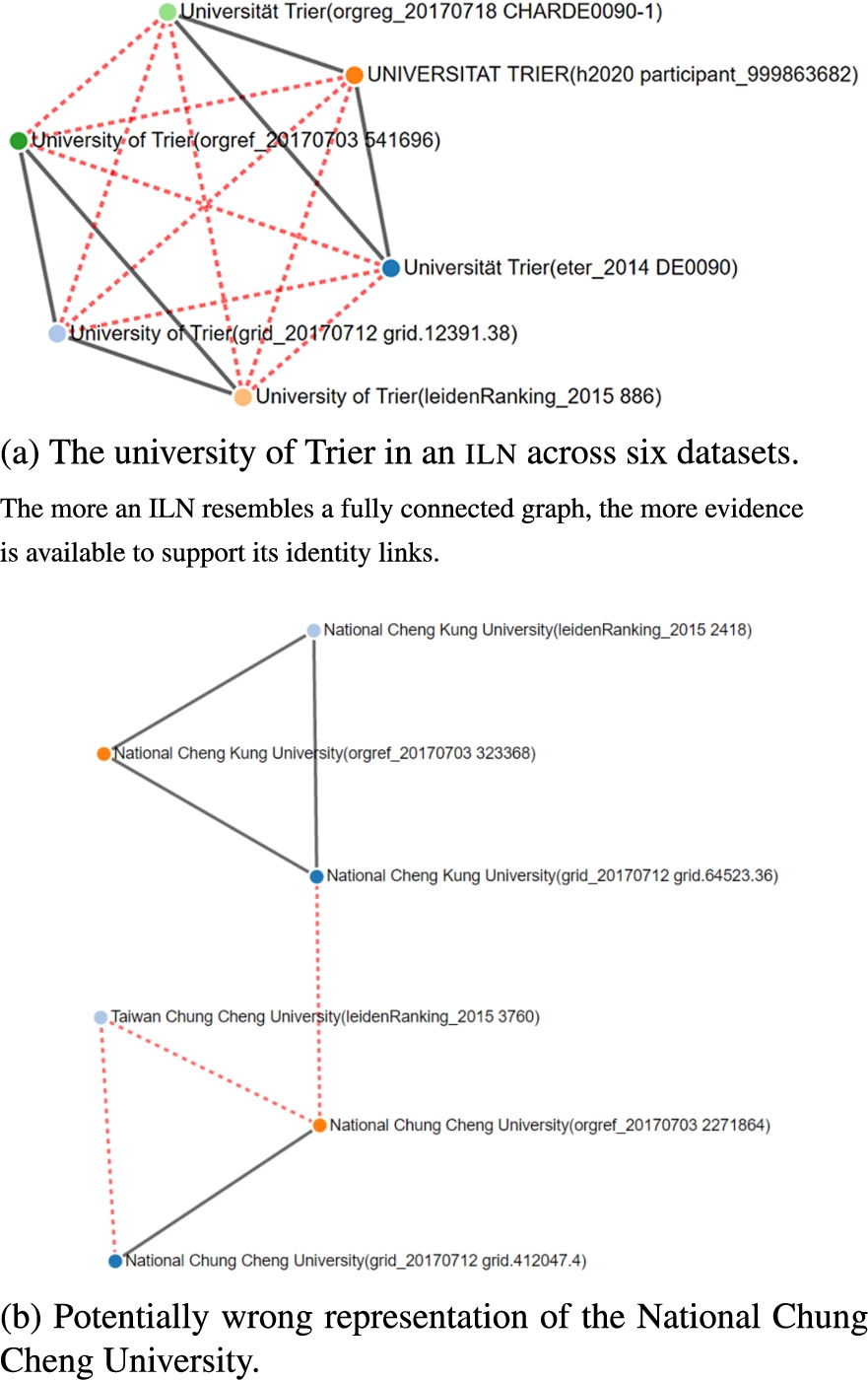
Two real life examples of identity link networks (ilns); dotted lines indicate links with a low confidence.

This paper begins with a short motivation in Section 2. Section 3 discusses the related work and Section 4 describes the proposed metric. In Section 6 we describe the datasets involved in our experiments. Sections 7 to 9 describe our three experiments. While Section 5 presents refinements of the proposed metric, Section 10 evaluates them and Section 11 concludes.

2. Identity link networks

We assume the well known setting of a real-world entity that has one or more digital representations in multiple datasets. The task of entity resolution is to discover which entity (or entities) in each dataset denotes the same real world entity. An Identity Link Network (iln) is a network of links between entities from a number of datasets that are found by one or more entity resolution algorithms to represent the same real world entity. An iln can be derived directly from entity resolution results (Sections 7 and 8), or it may be generated by sophisticated clustering methods as in our experiment in Section 9. In this work we do not propose any new entity resolution algorithm. Instead, we propose a method to automatically evaluate discovered links, particularly when they involve more than two datasets. Unfortunately, gold standards in initiatives such as OAEI3

³

http://oaei.ontologymatching.org/

do not go beyond two datasets.

Figure 1 shows two examples of such ilns that have been generated by an entity resolution algorithm between entities from six datasets taken from the field of Science, Technology and Innovation studies (STI) (more details in Section 6). Figure 1(a) shows the iln for the real world entity University of Trier, Fig. 1(b) shows the same for the National Chung Cheng University. In this paper, we hypothesise that the structure of theseilns is a reliable indicator for the correctness of the links in the network they form.

Algorithm 1:

Simple resource clustering algorithm & network documentation. All search, insertion and deletion within a cluster is supported with hash tables which allows for a complexity $\mathit{O}\mathrm{(}1\mathrm{)}$ leading the algorithm to be of $\mathit{O}\mathrm{(}\mathit{m}log\mathit{n}\mathrm{)}$ where m is the input size (number of links), n is the number of nodes and $\mathit{O}\mathrm{(}log\mathit{n}\mathrm{)}$ accounts for the worst case scenario where all first merged clusters are of size two. In detail, the worst case of the algorithm is when all links result in one cluster and require merging $\frac{\mathit{n}}{2}$ clusters of size two.

Simple clustering algorithm Our aim is not clustering, it is instead the quality approximation of ilns. So, for reproducibility purposes we present here the straight forward simple clustering algorithm (see Algorithm 1) implemented and used for clustering candidate linked resources in order to generate ilns. For the purpose of cluster quality estimation, the algorithm also documents the discovered links and their respective strength(s). By documenting more than one strength for a single link, the clustering algorithm enables the use of several matching algorithms. With this feature, for a link with strengths computed by different matching algorithms, the topmost strength is used for assessing the quality of an iln. All basic operations such as SEARCH (search for the cluster to which a node belongs), INSERTION (add a node to the set of nodes of a particular cluster, add a link to the set of links of a particular cluster, add a strength to the mapping link → strength of a particular cluster), and DELETION (deleting a cluster, reassign a cluster to a node) are supported by hash tables $\mathrm{(}\mathit{O}\mathrm{(}1\mathrm{)}\mathrm{)}$ . However, when accounting for the MERGING of clusters, its worst case scenario yields a complexity of $\mathit{O}\mathrm{(}log\mathit{n}\mathrm{)}$ where n is the number of nodes. This brings the overall time complexity to $\mathit{O}\mathrm{(}\mathit{m}log\mathit{n}\mathrm{)}$ in the worst case and $\mathit{O}\mathrm{(}\mathit{m}\mathrm{)}$ in the best case, where m is the size of the input or the number of links to be more precise. Figure 2 illustrates an application of Algorithm 1.

Fig. 2.

Example of link clustering using Algorithm 1. This example illustrates the creation and merging of clusters but leaves out the documentation of links and their strengths.

3. Related work

We briefly discuss a number of related areas from the literature, and indicate how our work differs from these in aim and scope.

Schema matching Much work in the literature focuses on ontology matching, especially schema matching [5]. Some rely on concept distance or an extended version of it [3,11,19]. Some rely on alignment similarities [4], others relies on formal logical conflicts between ontologies to detect and possibly repair mappings at a schema-level [10]. The current paper does not aim to match ontologies, nor does it critically rely on using ontological or schema information. We only assume the existence of external entity resolution algorithms for suggesting links between entities. Such algorithms may or may not exploit ontological information, but this does not affect our central hypothesis.

Information gain The work in [15] also uses network structure to evaluate link quality, but in a very different way. The main intuition there is that an individual link in an iln is more reliable when it leads to a greater information gain. The paper does not consider the structure of the iln as a whole, as we do in this paper.

Entity clustering Part of the literature also uses clustering of the digital representations of the same real world entity in one or multiple sources. While their data sources are mainly unstructured [1,2], our interest lies in clusters derived from the mappings of entities exclusively across knowledge-bases. In addition, they also do not consider the structure of the iln as a whole. Another part of the literature specifically focuses on clustering algorithms. The FAMER [14] framework for example provides and compares seven different link-based entity clustering approaches. The aim of our work is different from all of these. Whereas these works use clustering algorithms to construct entity resolutions, we show how a cluster-based metric can be used to assess the quality of a network of entity links, irrespective of how these links were generated.

Network metrics The work by Guéret et al. [6] is one of the few papers to our knowledge that uses network metrics to assess the quality of links. The key point that separates this work from ours is that it uses local network features, i.e. only the direct neighbours of a single node, while we employ global network features. [12] also addresses the same challenge. It evaluates a given cluster G by comparing it to a reference cluster R based on the number of splits and merges required to go from G to R. Our proposed metric does not need such a reference cluster, and is hence more easily applicable.

4. Network properties & quality of a link-network

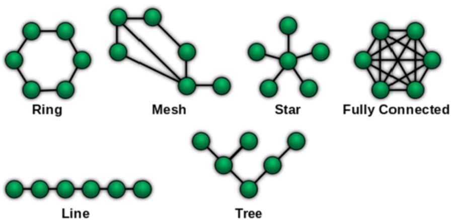
Figure 3 illustrates a set of six simple network topologies over the same number of nodes. Our proposed metric is based on the intuition that multiple links provide corroborating evidence for each other, suggesting that, in the case of an iln, the ideal topology is a fully connected network. It illustrates a total agreement between all resources (not the case for any other topology), and it does not require any intermediate resource to establish an identity-link between two resources (again, not the case for any other topology). Hence, intuitively, the amount of redundancy between paths in an iln is an indicator for the quality of the links in the iln. We will capture these and similar intuitions using three different global graph features over ilns: Bridge, Diameter and Closure.

Fig. 3.

Example of network topologies. Source: https://en.wikipedia.org/wiki/Network_topology.

We will now first define and explain the rationale behind each metric, then normalise each metric to values4

⁴

The metric value indicates the negative impact of one or more missing links in an iln.

between 0 and 1, and finally average the sum of all metrics to obtain the metric which we will use for estimating the quality of the iln.

Table 1

Metrics values for each of the topologies from Fig. 2

Bridge metric A bridge (also known as an isthmus or a cut-edge) in a graph is an edge whose removal increases the number of connected components of the graph, or equivalently, an edge that does not belong to any cycle. The intuition for this measure is that a bridge in an iln suggests a potentially problematic link which is not corroborated by any other links. As a graph with n nodes contains at most $\mathit{n}-1$ bridges (e.g. in a Line network), the bridge value is normalised as ${\mathit{n}}_{\mathit{b}}=\frac{\mathit{B}}{\mathit{n}-1}$ , where B is the number of bridges. An ideal link network would have no bridge ( ${\mathit{n}}_{\mathit{b}}=0$ ). As ${\mathit{n}}_{\mathit{b}}$ is sensitive to the total number of nodes in the graph (it decreases for large graphs, even when the number of bridges is constant), we “soften” the value of ${\mathit{n}}_{\mathit{b}}$ with a sigmoid function: ${\mathit{n}}_{\mathit{b}}^{\prime }=max\mathrm{(}{\mathit{n}}_{\mathit{b}}\mathrm{,}{sigmoid}_{\mathit{\eta }=1.6}\mathrm{(}\mathit{B}\mathrm{)}\mathrm{)}$ , where the function ${sigmoid}_{\mathit{\eta }=1.6}\mathrm{(}\mathit{x}\mathrm{)}=\frac{\mathit{x}}{|\mathit{x}|+\mathit{\eta }}$ helps stabilising the impact of the size of the graph by providing a minimal value for ${\mathit{n}}_{\mathit{b}}^{\prime }$ (see Section 9.1).

The value $\mathit{\eta }=1.6\text{ in }|\mathit{x}|+\mathit{\eta }$ at the denominator of the sigmoid function is a hyper-parameter that has been chosen not based on the data at hand but by qualitatively picking a gradual penalty that can be imposed on a network based on the number of times a particular rule has been broken. Thus, we do not claim that this value is optimal, we only show that this value is sufficient, and works across multiple experiments (see Section 9.1 were we further discuss the sigmoid function.)

Diameter metric The diameter D of a graph with n nodes is the maximum number of edges (distance) in a shortest path between any pair of vertices (i.e. the longest shortest path). In an ideal scenario, if three resources A, B and C are representations of the same real world object, there would be no need for an intermediate resource for confirming the identity of any of the resources in the network. In a fully connected graph of n nodes, each node is 1 edge-distance away from the rest, meaning that the diameter D has value 1. The longest diameter is observed in a Line network structure, with $\mathit{D}=\mathit{n}-1$ for a line network of n nodes. To scale to the $[0\mathrm{,}1]$ interval, the diameter is normalised as ${\mathit{n}}_{\mathit{d}}=\frac{\mathit{D}-1}{\mathrm{(}\mathit{n}-1\mathrm{)}-1}$ . Like the bridge, because the diameter is also sensitive to the number of nodes, the normalised diameter is calculated as ${\mathit{n}}_{\mathit{d}}^{\prime }=max\mathrm{(}{\mathit{n}}_{\mathit{d}}\mathrm{,}{sigmoid}_{\mathit{\eta }=1.6}\mathrm{(}\mathit{D}-1\mathrm{)}\mathrm{)}$ .

Closure metric In a connected graph of n nodes, the closure is the ratio of the number of arcs A in the graph over the total number of possible arcs $\frac{1}{2}\mathit{n}\mathrm{(}\mathit{n}-1\mathrm{)}$ . In a complete graph, this ratio has value 1. Hence, to evaluate how far the observed graph is from the ideal (complete) one, we normalise the closure metric as ${\mathit{n}}_{\mathit{c}}=1-\frac{\mathit{A}}{\frac{1}{2}\mathit{n}\mathrm{(}\mathit{n}-1\mathrm{)}}$ . The minimum number of connections is $\mathit{n}-1$ , as observed in Line and Star network structures.

Estimated quality metric All of these metrics capture the same intuition: the more an iln resembles a fully connected graph, the higher the quality of the links in the iln. Of course, these three metrics are not independent: ${\mathit{n}}_{\mathit{c}}=0$ or ${\mathit{n}}_{\mathit{d}}^{\prime }=0$ implies ${\mathit{n}}_{\mathit{b}}^{\prime }=0$ . However, using only ${\mathit{n}}_{\mathit{c}}$ or ${\mathit{n}}_{\mathit{d}}^{\prime }$ would be too uninformative since the converse of the implication does not hold. Table 1 shows that each of $n_c$ , $n_d^{\prime }$ and $n_b^{\prime }$ capture different (though related) amounts of redundancy in the iln and that each metric by itself fails to properly discriminate between the seven ilns depicted in Fig. 3. For example, ${\mathit{n}}_{\mathit{c}}$ and ${\mathit{n}}_{\mathit{b}}^{\prime }$ treat a Tree, Star and Line as qualitatively equal but disagree on whether a Full Mesh is as good as a Ring. Consequently, to compute an overall estimated quality $e_Q$ of an identity link network, we combine the three separate metrics by taking their average, and invert them so that the value 1 indicates the highest quality: $$\begin{array}{c}{e}_Q=1-{\displaystyle \frac{{\mathit{n}}_{\mathit{b}}^{\prime }+{\mathit{n}}_{\mathit{d}}^{\prime }+{\mathit{n}}_{\mathit{c}}}{3}}.\end{array}$$ In short, applying the $e_Q$ to a candidate identity link network assumes that all possible links are evaluated between resources across and within datasets of interest (see Fig. 5). So, the lack of one or more links is considered a potential evidence for suggesting the corresponding entities being different. This applies to identity graphs composed of more than two nodes (see Section 11.2 discussing network of size two).

Complexity The ${\mathit{e}}_{\mathit{Q}}$ metric is implemented using the NetworkX Python package. To evaluate the overall time complexity of the propose algorithm, we assess the complexity of each sub-metric: bridge, diameter and closure. (i) The last metric, the closure, is straightforward. It is an algebraic operation of computing the number of observed arcs over the space of possible arcs and therefore of O(1). (ii) According to the NetworkX documentation, the bridge implementation uses the Chain Decomposition algorithm5

⁵

An edge is a bridge if and only if it is not contained in any chain. In NetworkX, chains are found using the function chain_decomposition(). The documentation can be found at https://networkx.github.io/documentation/latest/reference/algorithms/generated/networkx.algorithms.bridges.bridges.html.

of [16] which is described to be of O(m + n) where n is the number of nodes in the graph and m is the number of edges. (iii) Computing the diameter metric appears to be the most time expensive. NetworkX documentation reports the diameter of a graph as the maximum eccentricity, where the eccentricity of a node v is the maximum distance from v to all other nodes in the graph. This therefore translates into computing all pairs shortest path lengths. Referring to the Johnson’s algorithm for computing all shortest path between each pair of nodes in a weighted graph, the complexity of computing the diameter of a graph is of O( ${\mathit{n}}^{2}log\mathit{n}+\mathit{n}\mathit{m}$ ), where n is the number of nodes and m the number of edges in the graph.

This indicates that the complexity of the ${\mathit{e}}_{\mathit{Q}}$ metric is of $\mathit{O}\mathrm{(}{\mathit{n}}^{2}log\mathit{n}+\mathit{n}\mathit{m}\mathrm{)}$ , which is a function of the size of the graph and the number of edges composing the graph. In reality, assuming that data-sources do not contain duplicates, the maximum size of an iln can be limited to the number of datasets involved. However, as this is a strong assumption to make over real data and because matching algorithms are not perfect, a candidate iln can unexpectedly reach a very big size. In general, a relatively big iln (with respect to the number of data-sources) often suggests the infiltration of false positive nodes and thereby suggesting a bad iln. To avoid unbearable waiting time for computing the ${\mathit{e}}_{\mathit{Q}}$ of large ilns, an upper bound can be set on the maximum size of candidate ilns.

Discrete intervals The ${\mathit{e}}_{\mathit{Q}}$ metric scores all ilns on a continuous value in the $[0\mathrm{,}1]$ interval. To automatically discriminate potentially good networks from bad ones, we divide this interval into three segments: ilns with values $0.9⩽{\mathit{e}}_{\mathit{Q}}⩽1$ will be rated as good , with values $0.75\mathrm{<}{\mathit{e}}_{\mathit{Q}}\mathrm{<}0.9$ as undecided , and with values $0⩽{\mathit{e}}_{\mathit{Q}}⩽0.75$ as bad . These boundaries are empirically determined, and can be adjusted depending on the use-case. The specific values of these boundaries do not affect the essence of our hypothesis.

Hypothesis.

We can now state our hypothesis more formally: “The ${\mathit{e}}_{\mathit{Q}}$ intervals defined above are predictive of the quality of the links in an entity link network between multiple datasets”.

Example.

By way of illustration, Table 1 gives the value of our ${\mathit{e}}_{\mathit{Q}}$ metric for the six networks from Fig. 3, and shows that the metric does indeed capture redundancy in a network.

In Sections 7 to 9, we will test this hypothesis against human evaluation on hundreds of ilns containing thousands of links in three experiments using between three to six datasets.

5. Refinements of ${\mathit{e}}_{\mathit{Q}}$ using link confidence scores produced by entity resolution algorithms

Given that all links have been searched for, the absence of a link in an iln network is shown to cripple the ideal structure of the network as it increases the chance for a longer diameter and the appearance of bridges, and it reduces the density of the network. These characteristics are thereby used by the ${\mathit{e}}_{\mathit{Q}}$ metric as a potential evidence for tagging as good or bad the network as a whole. Furthermore, the metric assumes a link correctness confidence score of 1 for all links in the network although it is not the case in the realm of entity matching unless a perfect match is found. Entity matching algorithms often produce pairwise matched entities with a confidence score in the interval $[0\mathrm{,}1]$ as a quantitative justification for the pair to be the same.

So far, we strictly estimate the quality of an identity network based on the cost of its missing links and thereby its structure. Now, the wonder lies in how to capture the toll of an existing link on estimating the quality of the network given that the link has a confidence score below one? In other words, is the strength of an identity link relevant in estimating the quality of the network using its structure?

To understand the importance of the strength of links in estimating the quality of an identity network using its structure, we propose three new network quality estimation metrics ( ${\mathit{e}}_{{\mathit{Q}}_{min}}$ , ${\mathit{e}}_{{\mathit{Q}}_{\mathrm{avg}}}$ and ${\mathit{e}}_{{\mathit{Q}}_{\mathit{w}}}$ ) that in their respective ways combine structure and link strength for network quality estimations. In Section 10 we evaluate these alternative metrics on the same ground truths used in Sections 7 to 9, and compare each one of them to the original ${\mathit{e}}_{\mathit{Q}}$ metric based on their respective ${\mathit{F}}_1$ scores in these various scenarios.

Before diving into the intricacies of link strength integration, we first start with the formalism that pave the way for understanding it.

A weighted, undirected, connected (WUC) graph6

⁶

We interchangeably refer to the undirected identity graph as network or cluster.

is defined as $\mathit{G}=\mathrm{(}\mathit{V}\mathrm{,}\mathit{L}\mathrm{,}\mathit{w}\mathrm{)}$ where V is the set of nodes, L is the set of links or edges, and $\mathit{w}:\mathit{L}\mapsto {\mathbb{R}}^{+}$ is a function mapping edges (unordered pair of vertices) ${\mathit{e}}_{\mathit{i}}=\mathrm{(}\mathit{u}\mathrm{,}\mathit{v}\mathrm{)}\in \mathit{L}$ – where $\mathit{u}\mathrm{,}\mathit{v}\in \mathit{V}$ for $\mathit{i}\in [1\mathrm{,}\mathit{k}]$ and k is the number of edges in G – to their decimal values $\mathit{w}\mathrm{(}{\mathit{e}}_{\mathit{i}}\mathrm{)}$ in the interval $[0\mathrm{,}1]$ . The weight of sub-graph $\mathit{H}\subset \mathit{G}$ is $\mathit{w}\mathrm{(}\mathit{H}\mathrm{)}={\sum }_{\mathit{e}\in \mathit{L}\mathrm{(}\mathit{H}\mathrm{)}}\mathit{w}\mathrm{(}\mathit{e}\mathrm{)}$ where $\mathit{L}\mathrm{(}\mathit{H}\mathrm{)}$ are the edges of H.

For two vertices a and $\mathit{b}\in \mathit{V}$ , a path between a and b is a sequence $\mathit{\pi }=\mathrm{(}{\mathit{e}}_1\mathrm{,}{\mathit{e}}_2\mathrm{,}\dots \mathrm{,}{\mathit{e}}_{\mathit{k}}\mathrm{)}$ where ${\mathit{e}}_{\mathit{i}}=\mathrm{(}{\mathit{v}}_{\mathit{i}-1}\mathrm{,}{\mathit{v}}_{\mathit{i}}\mathrm{)}\in \mathit{L}$ and ${\mathit{v}}_{\mathit{i}}\in \mathit{V}$ for $\mathit{i}\in [1\mathrm{,}\mathit{k}]$ where k is the number of edges in π, with ${\mathit{v}}_{\mathit{o}}=\mathit{a}$ and ${\mathit{v}}_{\mathit{k}}=\mathit{b}$ . $\mathrm{\Pi }\mathrm{(}\mathit{a}\mathrm{,}\mathit{b}\mathrm{)}$ denotes the set of all paths from a to b. The geodesic distance and weighted geodesic distance between a and b are respectively given by Eqs (1) and (2) $$\begin{array}{}\text{(1)}& dist\mathrm{(}\mathit{a}\mathrm{,}\mathit{b}\mathrm{)}=\underset{\mathit{\pi }\in \mathrm{\Pi }\mathrm{(}\mathit{a}\mathrm{,}\mathit{b}\mathrm{)}}{min}|\mathit{\pi }|\text{(2)}& {dist}_{\mathit{w}}\mathrm{(}\mathit{a}\mathrm{,}\mathit{b}\mathrm{)}=\underset{\mathit{\pi }\in \mathrm{\Pi }\mathrm{(}\mathit{a}\mathrm{,}\mathit{b}\mathrm{)}}{min}{\displaystyle \sum }_{\mathit{e}\in \mathit{\pi }}\mathit{w}\mathrm{(}\mathit{e}\mathrm{)}\end{array}$$ and the diameter and weighted diameter of G are given by Eqs (3) and (4) $$\begin{array}{}\text{(3)}& diam\mathrm{(}\mathit{G}\mathrm{)}=\underset{\mathit{a}\mathrm{,}\mathit{b}\in \mathit{V}}{max}dist\mathrm{(}\mathit{a}\mathrm{,}\mathit{b}\mathrm{)}\text{(4)}& {diam}_{\mathit{w}}\mathrm{(}\mathit{G}\mathrm{)}=\underset{\mathit{a}\mathrm{,}\mathit{b}\in \mathit{V}}{max}{dist}_{\mathit{w}}\mathrm{(}\mathit{a}\mathrm{,}\mathit{b}\mathrm{)}\end{array}$$ We now have the prerequisites in place for presenting three hybrid ways of integrating link strength into the proposed network quality estimation metric.

5.1. Weakest link

In this approach, we define ${\mathit{e}}_{{\mathit{Q}}_{min}}$ as the metric to estimate the quality of an identity network G based on both the structure of G and the strength of the links composing G. ${\mathit{e}}_{{\mathit{Q}}_{min}}$ is computed as the product of the original ${\mathit{e}}_{\mathit{Q}}$ score and the weakest link strength in the network as given by Eq. (5). $$\begin{array}{}\text{(5)}& {\mathit{e}}_{{\mathit{Q}}_{min}}={\mathit{e}}_{\mathit{Q}}\times \underset{\mathit{e}\in \mathit{L}\mathrm{(}\mathit{G}\mathrm{)}}{min}\mathit{w}\mathrm{(}\mathit{e}\mathrm{)}\end{array}$$

5.2. Link average

Compared to the first weight integration approach, here, we simply replace the weakest link strength of G by the average of all strengths in G to obtain ${\mathit{e}}_{{\mathit{Q}}_{\mathrm{avg}}}$ as provided in Eq. (6). $$\begin{array}{}\text{(6)}& {\mathit{e}}_{{\mathit{Q}}_{\mathrm{avg}}}={\mathit{e}}_{\mathit{Q}}\times {\displaystyle \frac{{\sum }_{\mathit{e}\in \mathit{L}\mathrm{(}\mathit{G}\mathrm{)}}\mathit{w}\mathrm{(}{\mathit{e}}_{\mathit{i}}\mathrm{)}}{|\mathit{L}\mathrm{(}\mathit{G}\mathrm{)}|}}\end{array}$$

5.3. Rooted link

As opposed to the first two approaches where we integrate the link strength without modifying the initial ${\mathit{e}}_{\mathit{Q}}$ computation, here, we do the opposite. We use the link confidence score for computing each sub-metric score (bridge, diameter and closure). Doing so, the link confidence score is now more rooted into the initial ${\mathit{e}}_{\mathit{Q}}$ formulation, leading to its equation adjustment. The detail on how the ${\mathit{e}}_{\mathit{Q}}$ formula is adjusted for integrating the link’s strength leading to Equation (10) is provided in the next paragraphs.

Weighted bridge metric Given an identity graph G with n nodes, the idea here is to capture the softening of the bridge metric measure as the strength of the edges composing the set of bridges in G weaken. This is formulated in Equation (7): the weaker the strength of a bridge gets, the less it negatively affects the quality of an identity network.

The approach may sound counter-intuitive, specially if one expects the quality estimation of a graph G to correlate positively with the strength of its edges. This, under the assumption that the strength of the bridge-edge(s) is the only available evidence for considering identical the nodes in the identity graph.

However, with respect to the presence of one or more bridges in a graph, our proposal assumes the opposite. Take for example Fig. 1(b) where the two components of the graph (different universities) are connected by a bridge. Here, as we take the existence of the bridge as an indication that the graph should be partitioned into isolated components, then we shall agree that generating a bridge with a high strength for connecting isolated components is more damaging than a bridge with a weak strength. In short, a bridge should be seen as a penalty, not a reward hence its strength negatively correlates with the graph’s quality. In Fig. 4(b), for example, the maximum penalty for having three strong (unweighted) bridges in the star network is 1 whereas it is in fact 0.57 as the majority of the bridge-edges are weak.

Fig. 4.

Examples of ${\mathit{e}}_{\mathit{Q}}$ values for two weighted ILNs.

The weighted bridge metric ${\mathit{n}}_{{\mathit{b}}_{\mathit{w}}}^{\prime }\mathrm{(}\mathit{G}\mathrm{)}$ of a graph G is the maximum between the normalisation of the weighted bridges ${\mathit{n}}_{{\mathit{b}}_{\mathit{w}}}\mathrm{(}\mathit{G}\mathrm{)}$ of the graph and the sigmoid of the sum of the weighted bridges $\mathit{w}\mathrm{(}\mathit{B}\mathrm{)}$ of the graph. $$\begin{array}{}\text{(7)}& {\mathit{n}}_{{\mathit{b}}_{\mathit{w}}}^{\prime }\mathrm{(}\mathit{G}\mathrm{)}=max\mathrm{(}{\mathit{n}}_{{\mathit{b}}_{\mathit{w}}}\mathrm{(}\mathit{G}\mathrm{)}\mathrm{,}sigmoid\mathrm{(}\mathit{w}\mathrm{(}\mathit{B}\mathrm{)}\mathrm{\left)}\mathrm{\right)}\end{array}$$ where B is defined as sub-graph(s) of G whose edges are the bridges in G and $$\begin{array}{c}{\mathit{n}}_{{\mathit{b}}_{\mathit{w}}}\mathrm{(}\mathit{G}\mathrm{)}={\displaystyle \frac{\mathit{w}\mathrm{(}\mathit{B}\mathrm{)}}{\mathit{n}-1}}={\displaystyle \frac{{\sum }_{\mathit{e}\in \mathit{L}\mathrm{(}\mathit{B}\mathrm{)}}\mathit{w}\mathrm{(}\mathit{e}\mathrm{)}}{\mathit{n}-1}}\end{array}$$

Weighted diameter metric Defined in Equation (8), the weighted diameter metric ${\mathit{n}}_{{\mathit{d}}_{\mathit{w}}}^{\prime }\mathrm{(}\mathit{G}\mathrm{)}$ includes strength by elongating the unweighted geodesic distance $eDiam\mathrm{(}\mathit{G}\mathrm{)}$ of G as the edges composing it weaken in strength. In other words, the smaller the strength, the longer the diameter gets. This allows us to predict the decrease of the quality of an identity network whenever its diameter increases. It furthermore allows to increase the decrease of the quality of the identity network with respect to the weakening of the strength of each edge composing the network’s diameter. In Equation (8), ${\mathit{n}}_{{\mathit{d}}_{\mathit{w}}}^{\prime }\mathrm{(}\mathit{G}\mathrm{)}$ is then the maximum between the normalisation of the weighted diameter ${\mathit{n}}_{{\mathit{d}}_{\mathit{w}}}\mathrm{(}\mathit{G}\mathrm{)}$ of the graph and the sigmoid of the elongated diameter $eDiam\mathrm{(}\mathit{G}\mathrm{)}-1$ . $$\begin{array}{rcl}{\mathit{n}}_{{\mathit{d}}_{\mathit{w}}}^{\prime }\mathrm{(}\mathit{G}\mathrm{)}& =& max\mathrm{(}{\mathit{n}}_{{\mathit{d}}_{\mathit{w}}}\mathrm{(}\mathit{G}\mathrm{)}\mathrm{,}\\ \text{(8)}& & & sigmoid\mathrm{(}eDiam\mathrm{(}\mathit{G}\mathrm{)}-1\mathrm{)}\mathrm{)}\end{array}$$ where $eDiam\mathrm{(}\mathit{G}\mathrm{)}=2diam\mathrm{(}\mathit{G}\mathrm{)}-{diam}_{\mathit{w}}\mathrm{(}\mathit{G}\mathrm{)}$ and $$\begin{array}{c}{\mathit{n}}_{{\mathit{d}}_{\mathit{w}}}\mathrm{(}\mathit{G}\mathrm{)}=\left\{\begin{array}{cc}1\hfill & \text{if }eDiam\mathrm{(}\mathit{G}\mathrm{)}\mathrm{>}\mathit{n}-2\hfill \\ \frac{eDiam\mathrm{(}\mathit{G}\mathrm{)}}{\mathrm{(}\mathit{n}-1\mathrm{)}-1}\hfill \end{array}\right.\end{array}$$

Weighted closure metric This last metric ${\mathit{n}}_{{\mathit{c}}_{\mathit{w}}}\mathrm{(}\mathit{G}\mathrm{)}$ is computed by inverting the normalised sum of the weighted edges $\mathit{w}\mathrm{(}\mathit{G}\mathrm{)}$ of G as provided in Equation (9). $$\begin{array}{rcl}{\mathit{n}}_{{\mathit{c}}_{\mathit{w}}}\mathrm{(}\mathit{G}\mathrm{)}& =& 1-{\displaystyle \frac{\mathit{w}\mathrm{(}\mathit{G}\mathrm{)}}{\frac{1}{2}\mathit{n}\mathrm{(}\mathit{n}-1\mathrm{)}}}\\ \text{(9)}& & =& 1-{\displaystyle \frac{{\sum }_{\mathit{e}\in \mathit{L}}\mathit{w}\mathrm{(}\mathit{e}\mathrm{)}}{\frac{1}{2}\mathit{n}\mathrm{(}\mathit{n}-1\mathrm{)}}}\end{array}$$

We are now able to compute a weighted ${\mathit{e}}_{\mathit{Q}}$ as defined in Equation (10). Observe that each of the three metrics outputs a score in the interval $[0\mathrm{,}1]$ . Therefore, the overall measure is also in the interval $[0\mathrm{,}1]$ . $$\begin{array}{}\text{(10)}& e_{Q_w}\mathrm{(}\mathit{G}\mathrm{)}=1-{\displaystyle \frac{{\mathit{n}}_{{\mathit{b}}_{\mathit{w}}}^{\prime }\mathrm{(}\mathit{G}\mathrm{)}+{\mathit{n}}_{{\mathit{d}}_{\mathit{w}}}^{\prime }\mathrm{(}\mathit{G}\mathrm{)}+{\mathit{n}}_{{\mathit{c}}_{\mathit{w}}}\mathrm{(}\mathit{G}\mathrm{)}}{3}}\end{array}$$

Examples.

For a better understanding of these measures, let us assume two networks A and B with three edges (see Fig. 4). A with 3 nodes is a complete network and B with 4 nodes is a star network. For each network, the edges’ strengths are respectively $\mathit{w}\mathrm{(}{\mathit{e}}_1\mathrm{)}=0.9$ , $\mathit{w}\mathrm{(}{\mathit{e}}_2\mathrm{)}=0.5$ and $\mathit{w}\mathrm{(}{\mathit{e}}_3\mathrm{)}=0.3$ . Regardless of the strength in each network, the unweighted bridge, diameter and closure metrics’ values for A and B are respectively ${\mathit{n}}_{\mathit{b}}\mathrm{(}\mathit{A}\mathrm{)}=\frac{0}{3-1}=0$ and ${\mathit{n}}_{\mathit{b}}\mathrm{(}\mathit{B}\mathrm{)}=\frac{3}{4-1}=1$ ; ${\mathit{n}}_{\mathit{d}}\mathrm{(}\mathit{A}\mathrm{)}=\frac{1-1}{3-2}=0$ and ${\mathit{n}}_{\mathit{d}}\mathrm{(}\mathit{B}\mathrm{)}=\frac{2-1}{4-2}=0.5$ ; ${\mathit{n}}_{\mathit{c}}\mathrm{(}\mathit{A}\mathrm{)}=1-\frac{3}{3}=0$ and ${\mathit{n}}_{\mathit{c}}\mathrm{(}\mathit{B}\mathrm{)}=1-\frac{3}{6}=0.5$ while their weighted bridge, diameter and closure metrics’ values are ${\mathit{n}}_{{\mathit{b}}_{\mathit{w}}}\mathrm{(}\mathit{A}\mathrm{)}=\frac{0}{3-1}=0$ and ${\mathit{n}}_{{\mathit{b}}_{\mathit{w}}}\mathrm{(}\mathit{B}\mathrm{)}=\frac{0.9+0.3+0.5}{4-1}=\frac{1.7}{4-1}=0.57$ ; ${\mathit{n}}_{{\mathit{d}}_{\mathit{w}}}\mathrm{(}\mathit{A}\mathrm{)}=\frac{2-0.3-1}{3-2}=\frac{0.7}{1}=0.7$ and ${\mathit{n}}_{{\mathit{d}}_{\mathit{w}}}\mathrm{(}\mathit{B}\mathrm{)}=\frac{4-\mathrm{(}0.3+0.5\mathrm{)}-1}{4-2}=\frac{2.2}{2}=1.1$ but converted to 1; ${\mathit{n}}_{{\mathit{c}}_{\mathit{w}}}\mathrm{(}\mathit{A}\mathrm{)}=|1-\frac{0.9+0.5+0.3}{3}|=|1-\frac{1.7}{3}|=0.43$ and ${\mathit{n}}_{{\mathit{c}}_{\mathit{w}}}\mathrm{(}\mathit{B}\mathrm{)}=|1-\frac{0.9+0.5+0.3}{6}|=|1-\frac{1.7}{6}|=0.72$ . This example illustrates among others that the weaker the edges of a diameter, the longer the weighted diameter.

6. Datasets

We considered using datasets and gold standards from the OAEI initiative, but none of these go beyond links between two datasets. We therefore created our own gold standard on realistic datasets taken from the domain of social science, more specifically from the field of Science, Technology and Innovation (STI) studies. We consider this to be an important contribution of this paper. All datasets and our gold standard are available online at the locations given in later paragraphs.

Entities of interest to the STI domain of study are (among others) universities and other research-related organisations, such as R&D companies and funding agencies. Our six datasets are widely used in the field, and describe organisations and their properties such as name, location, type, size and other features.7

⁷

The information provided here about the datasets was collected in January 2018. The datasets themselves are of earlier dates: Grid: 2017.07.12; Orgref: 2017.07.03; OpenAire: 2017.08.16; OrgReg: 2017.07.18; Eter: 2014; Leiden Ranking 2015: 2017.6.16; and Cordis-H2020: 2016.12.22. All these datasets are available on the RISIS platform at http://datasets.risis.eu/.

Grid8

⁸

https://www.grid.ac

describes 80248 organisations across 221 countries using 12308 relationships. All organisations are assigned an address, while 96% of them have an organisation type, and only 78% have geographic coordinates.

OrgRef9

⁹

http://www.orgref.org

collates data about the most important worldwide academic and research organisations (31000) from two main sources: Wikipedia and ISNI.

The Leiden Ranking dataset10

¹⁰

http://www.leidenranking.com/

offers scientific performance indicators of more than 900 major universities. These universities are only included when they are above the threshold of 1000 fractionally counted Web of Science indexed core publications. This explains its coverage across only 54 worldwide countries.

Eter11

¹¹

https://www.eter-project.com/

is a database on European Higher Education Institutions that not only includes research universities, but also colleges and a large number of specialized schools. The dataset covered 35 countries in 2015.

OrgReg12

¹²

http://risis.eu/orgreg/

is based on Eter but adds to the about 2700 higher education institutions some 500 public research organizations and university hospitals. Collected between 2000 and 2016, its organisations are distributed across 36 countries.

The European Organisations’ Projects H2020 database13

¹³

http://www.gaeu.com/sv/item/horizon-2020

documents the Horizon 2020 participating organisations.

7. ${\mathit{e}}_{\mathit{Q}}$ put to the test

We test our hypothesis on a real life case study that revolves around the six datasets described in Section 6, with the goal to investigate the coverage of OrgReg (coverage analysis of datasets is a typical question asked by social scientists before including a dataset in their studies). This is done by comparing the entities in OrgReg to those in the other five datasets (Fig. 5).

Fig. 5.

Disambiguating OrgReg.

Fig. 6.

Overview of the generated identity link networks.

Table 2

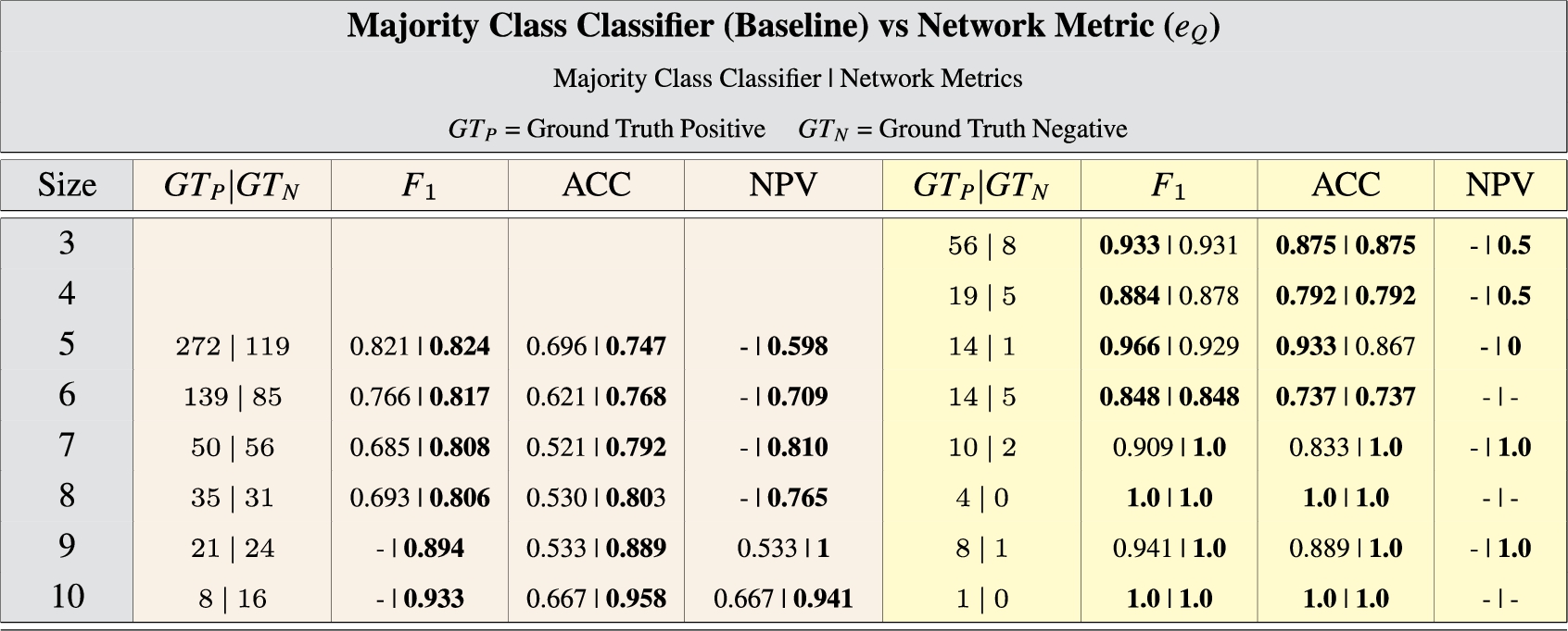
Majority class classifier baseline against the ${\mathit{e}}_{\mathit{Q}}$ metric using non expert ground truth (left), and expert sampled ground truth (right)

7.1. Experiment design

Organisations are linked across or within datasets using an approximate string matching on their names with a minimal similarity threshold of 0.8. Based on this, we generate links between each pair of datasets, resulting in 21 sets of links (including linking a dataset to itself in order to detect duplicate entities in the dataset). We then take the union of all 21 sets of links, resulting in a collection of iln’s of varying size using Algorithm 1 (see Fig. 6).

Now that we have constructed a large collection of multi-dataset ilns, we will compute the ${\mathit{e}}_{\mathit{Q}}$ value for all of them. Then, the machine-predicted good/bad categories (using ${\mathit{e}}_{\mathit{Q}}$ ) will be checked against the ground truth by a non-domain expert (the first author of this paper) and further verified by a domain expert (the third author). This ground truth is available online. In the ground truth, a candidate iln is classified as positive (good) only if all nodes in the network are co-referent (all resources point to the same real-life object), regardless of whether the network is complete (full mesh network) or not. Whenever the resources in the network point to more than one real life object, the network is classified as negative (bad).

Notice that we have deliberately used a very weak entity resolution algorithm in this experiment (approximate string matching). This produces links of both very high and rather low quality, providing a genuine test for our ${\mathit{e}}_{\mathit{Q}}$ metric to distinguish between them.

7.2. Results of first evaluation (non expert)

Ideally, we would find only ilns of size 6 if each OrgReg entity were linked with one and only one entity in each of the five other datasets. With less than 100% coverage of OrgReg, we also expect to find ilns of size smaller than 6. Figure 6 shows that we also find a substantial number of ilns of size bigger than 6. This is due to (i) duplicates occurring in a single dataset, resulting in links in the iln between two items from the same dataset, and (ii) an imperfect matching algorithm (in our case approximate name matching), resulting in incorrect links in the iln.

Due to the high number of ilns generated,14

¹⁴

On a 6th Gen Intel^® Core^TM i7 notebook with 8GB RAM, it takes about 100 seconds to automatically evaluate all 4398 clusters of size three and above (see Fig. 6).

we evaluate only the 846 ilns of size 5 to 10, with the following frequencies: 391 (size 5), 224 (6), 96 (7), 66 (8), 45 (9) and 24 (10). We predict a good or bad score based on the ${\mathit{e}}_{\mathit{Q}}$ interval values for each of the 846 ilns, and then compare the scores against those of a human judge, resulting in ${\mathit{F}}_1$ scores. In red, Fig. 6 displays the ${\mathit{F}}_1$ value for each iln size. Overall, our ${\mathit{e}}_{\mathit{Q}}$ metric resulted in high ${\mathit{F}}_1$ values ( $0.806⩽{\mathit{F}}_1⩽0.933$ ). We also pitched our ${\mathit{e}}_{\mathit{Q}}$ metric against a Majority Class Classifier, which automatically classifies all identity link networks as good if the majority of networks are positive according to the human judges or classifies them all as bad otherwise. Table 2 shows that our ${\mathit{e}}_{\mathit{Q}}$ metric outperforms the Classifier on ${\mathit{F}}_1$ measure, Accuracy (ACC) and Negative Predicted Value (NPV) for ilns of all sizes.

All of these findings show the very strong predictive power of our ${\mathit{e}}_{\mathit{Q}}$ metric for the quality of ilns when compared to human judgement.

7.3. Results of second evaluation (expert)

Preferably, all results should be evaluated by domain experts. Realistically, this is not feasible. To show, however, that the evaluation by non-experts is not biased and mostly reliable, we include the validation of an expert by having him validate the fraction of the results for which he has the expertise. Therefore, a Dutch domain expert from the field of STI (the third author of this paper), was given the fraction of 148 ilns (ranging from size 3 to 10 as depicted in Table 2) in which at least one entity is located in the Netherlands. The expert deviated from the first evaluation in only 12 out of 148 cases. Although the changes slightly affect the ground truth for each iln size, the ${\mathit{F}}_1$ values computed here are even higher ( $0.848⩽{\mathit{F}}_1⩽1$ ) as compared to the previous experiment. This shows that the non-expert nature of the first human judgement was not detrimental to our results.15

¹⁵

However, the very imbalanced character of the ground truth makes it hard to always outperform the baseline as illustrated in Table 2.

This second experiment confirms our finding in the first experiment that ${\mathit{e}}_{\mathit{Q}}$ is a reliable predictor of iln quality.

7.4. Analysis

Both of the evaluations of ${\mathit{e}}_{\mathit{Q}}$ above resulted in very high ${\mathit{F}}_1$ average values of 0.847 and 0.948 respectively. Furthermore, ${\mathit{e}}_{\mathit{Q}}$ outperformed a majority-class classifier in the first experiment (not in the second because of the highly imbalanced distribution). All this supports our hypothesis that our ${\mathit{e}}_{\mathit{Q}}$ measure is strongly predictive of the quality of the links between the entities in an Identity Link Network.

8. ${\mathit{e}}_{\mathit{Q}}$ estimations in noisy settings

The previous experiment created links between entities using a rather weak entity resolution heuristic. This was an interesting setting because such weak matching strategies are a fact of daily life on the semantic web (and in data integration in general). In the next experiment, we will use ${\mathit{e}}_{\mathit{Q}}$ to evaluate iln’s that have been constructed using a more sophisticated matching heuristic, where we can control the amount of incorrect links in the ilns. We will see that also in this case, ${\mathit{e}}_{\mathit{Q}}$ is strongly predictive of human judged link quality.

The stronger matching heuristic that we use in this second experiment combines organisation names with the geo-location of the organisation. The experiment is run over Eter, Grid and OrgReg as they are the only datasets at our disposal that contain such geo-coordinates for organisations. To test the performance of the ${\mathit{e}}_{\mathit{Q}}$ metric at various levels of noise, we implement three sub-experiments where noise (the number of false positive links) is introduced by decreasing the name similarity threshold from 0.8 (experiment 1) to 0.7 and by increasing the geographic proximity distance threshold as described in the next sub-section.

8.1. Experiment design

This subsection describes in three phases how the experiment is conducted.

Phase-1: Create links The first phase links organizations across the three datasets whenever they are located within a radius of 50 meters, 500 meters and 2 kilometres. This creates nine sets of links (three for each radius).

Phase-2: Refine links Each set of links is then refined by applying an approximate name comparison over the linked resources with a threshold of 0.7.

By now, we have geo-only (without name comparison) and geo+names sets of links, organised in three subgroups (50 m, 500 m and 2 km) each.

Phase-3: Combine links To generate the final ilns, the sets of links within each subgroup are combined using the union operator. The goal of this is to compare, within a specified distance, ilns that where generated without name matching to those generated with name matching.

Choice of parameters threshold: in the previous experiment, the threshold of 0.8 is set relatively high to compensate for using only ‘name’ as means to validate resources, which has a low discriminative power. In this second experiment, because the name similarity is combined with geolocation, the threshold is dropped by 0.1 hoping for the geolocation to correct obvious noise due to the lower threshold of 0.7. As with the choice of the sigmoid parameter in Section 4, we do not make any optimality claim about this parameter, but only show that our qualitative choice is already sufficient to obtain good results.

vicinity of 50 m, 500 m and 2 km: these numbers are chosen to observe their influence on the quality of the network generated under each condition. The expectation is that, by increasing the vicinity distance we anticipate an increase in the number of false positive links (noise) and we want to test if the ${\mathit{e}}_{\mathit{Q}}$ metric will highlight potentially problematic ilns.

8.2. Strict vs. liberal clustering

To understand how link-networks are formed as we increase the geo-similarity distance, Fig. 7 illustrates how ilns may evolve as we move from strict constraints (scenario 1) to liberal constraints (scenario 3). First, in scenario 1, four ilns are derived from the six links: ${\mathit{c}}_1=\{⟨{\mathit{a}}_1⟩\mathrm{,}⟨{\mathit{b}}_3⟩\}$ , ${\mathit{c}}_2=\{⟨{\mathit{a}}_3⟩\mathrm{,}⟨{\mathit{b}}_1⟩\}$ , ${\mathit{c}}_3=\{⟨{\mathit{a}}_4⟩\mathrm{,}⟨{\mathit{b}}_4⟩\}$ and ${\mathit{c}}_4=\{⟨{\mathit{a}}_5⟩\mathrm{,}⟨{\mathit{b}}_6\mathrm{,}{\mathit{b}}_8\mathrm{,}{\mathit{b}}_9⟩\}$ . Then, the new link between ${\mathit{a}}_3$ and ${\mathit{b}}_3$ in scenario 2 forces ${\mathit{c}}_1$ and ${\mathit{c}}_2$ to merge . We now have a total of three ilns: ${\mathit{c}}_1=\{⟨{\mathit{a}}_1\mathrm{,}{\mathit{a}}_3⟩\mathrm{,}⟨{\mathit{b}}_1\mathrm{,}{\mathit{b}}_3⟩\}$ , ${\mathit{c}}_3=\{⟨{\mathit{a}}_4⟩\mathrm{,}⟨{\mathit{b}}_4⟩\}$ and ${\mathit{c}}_4=\{⟨{\mathit{a}}_5⟩\mathrm{,}⟨{\mathit{b}}_6\mathrm{,}{\mathit{b}}_8\mathrm{,}{\mathit{b}}_9⟩\}$ . Finally, in scenario 3, two new links appear. The first link between ${\mathit{a}}_4$ and ${\mathit{b}}_6$ causes the merging of ${\mathit{c}}_3$ and ${\mathit{c}}_4$ while the second link connecting ${\mathit{a}}_6$ to ${\mathit{b}}_2$ causes the creation of a new iln. Thereby, the total number of ilns remains 3.

Fig. 7.

Decrease/increase of ilns a line pattern is associated to each cluster. The non-black line colours (red and cyan) in scenarios 2 and 3 indicate the inclusion of a new links between resources.

These scenarios show that, as the iln constraints become more liberal, the number of links discovered increases while the number of ilns may increase, remain equal, or even decrease. In other words, when the matching conditions become liberal or less strict, two types of event may happen: (1) formation of new ilns and/or (2) merging of ilns. Table 3, shows that, in experiment 2, phenomenon (1) overtakes (2), which explains the increase in the number of ilns as the near-by distance increases.

Table 3

Link-network overview

8.3. Result and analysis

Respectively, Fig. 8.a and 8.b show the distribution of ilns using geo-only and geo+names methods.16

¹⁶

Bins of size two are omitted as they are too large to be plotted together with the rest of the histogram bars.

When combined, resource’s vicinity and name reduce the ilns bins to mostly sizes 2 and 3 as shown in Fig. 8.b.

Fig. 8.

Overview of the generated identity link networks.

Overall, as illustrated in Table 3, the number of ilns generated in this experiment increases with the increase of the geo-similarity radius. Within a radius of 50 meters, a total of 230 ilns are generated based on geo-distance only. This number reached 841 ilns at a 2 kilometres radius. After performing name matching, many links are pruned. Depending on the matching radius, the number of ilns varies from 36 to 371.

Due to manpower limitations we restrict our evaluation efforts to networks of size 3. These ilns cover 86% of the overall ilns ( $\mathit{size}\mathrm{>}2$ ) within 50 m radius and 92% within 500 m and 2 km radius. Table 4 shows the results of pitching our ${\mathit{e}}_{\mathit{Q}}$ metric against the human evaluation of the ilns under both the geo-only and the geo+names conditions.

Table 4

Automated flagging versus human evaluation

Table 5

Confusion matrix for ILNs of size 3, 2 km, geo-only

Table 6

Confusion matrix for ilns of size 3, 2 km, geo+names

Table 7

Network-metric ( ${\mathit{e}}_{\mathit{Q}}$ ) result versus the MCC baseline

As an example, the values ${\mathit{F}}_1=0.803$ and ${\mathit{F}}_1=0.912$ respectively depicted in the confusion matrices in Table 5 and Table 6 detail the machine quality judgements versus human evaluations of the networks generated within 2 kilometres radius under respectively geo-only and geo+names conditions.17

¹⁷

All confusion matrices supporting the analysis can be found at https://tinyurl.com/confusion-matrices.

Analysis In this experiment, we test the behaviour of the proposed ${\mathit{e}}_{\mathit{Q}}$ metric in both noisy (proximity only) and noise-less (proximity plus name) scenarios. The proposed ${\mathit{e}}_{\mathit{Q}}$ metric is in general able to exclude poor networks in noisy environments and to include good networks in noise-less environments. In addition, on the one hand, the relatively low ${\mathit{F}}_1$ measures displayed in Table 7 in noisy scenarios, highlight that proximity alone is not a good enough identity criterion for the data at hand. On the other hand, the relatively high ${\mathit{F}}_1$ measures in noise-less scenarios is an indication of stability and consistency that is in line with results outlined in experiment 1.

The results depicted in Table 7 show an uneven distribution of the candidate-sets. In a relatively balanced candidate-set scenario, our approach works well as can be seen in the first experiment and in the proximity only scenario. However, even though in extreme cases (proximity plus name) the Majority Class Classifier takes the lead, the network metric does not fall far behind. It is important to realise that our network metric does it with without knowing what the majority class is, knowledge that the Majority Class Classifier is of course privy to.

As in the first experiment, for further evaluation, we extracted a sample based on ilns in which at least one organisation originates from the Netherlands. Out of the 107 sampled ilns, the domain expert deviated from the first evaluation in only 1 case.

9. ${\mathit{e}}_{\mathit{Q}}$ put to a ranking test

The authors of the recently published paper [14] compared seven algorithms (clip, ccpivot, center, concom, mcenter, star1, star2) for clustering entities from multiple sources at different string similarity thresholds (0.75, 0.80, 0.85, 0.90). They evaluated the quality of the clusters generated by these algorithms on three gold standard datasets,18

¹⁸

https://dbs.uni-leipzig.de/de/research/projects/object_matching/famer

one manually built (referred here as GT1), and two syntactically generated. We take the evaluation results from [14] on GT1, and then test if our ${\mathit{e}}_{\mathit{Q}}$ score is able to correctly predict the ranking of the algorithms as found in the reported evaluation. In contrast to the earlier experiments (where we use ${\mathit{e}}_{\mathit{Q}}$ to assess the quality of clusters), we are now testing if ${\mathit{e}}_{\mathit{Q}}$ can be used to correctly rank different clustering algorithms across datasets.

Fig. 9.

Evaluation of ${\mathit{e}}_{\mathit{Q}}$ on the ranking from [14].

A slightly complicating factor is that the evaluation in [14] relies on ${\mathit{F}}_1$ values computed on true pairs of entities found. Since ${\mathit{e}}_{\mathit{Q}}$ evaluates on a per cluster basis (i.e. sets of more than two pairs of entities ( $\mathit{S}\mathrm{>}2$ )) and not on individual pairs, we recompute the ${\mathit{F}}_1$ values based on true clusters found ( $\mathit{S}\mathrm{>}2$ ) and plot these performance measures for each algorithm in Fig. 9 as Baseline. The resulting plot is comparable to the original one in [14]. We then run the ${\mathit{e}}_{\mathit{Q}}$ metric over the outputs of each algorithm at the same thresholds, displayed in Fig. 9 as ${\mathit{e}}_{\mathit{Q}}$ Evaluation. Looking at the result with bare eye, it shows that the ranking of the algorithms by ${\mathit{e}}_{\mathit{Q}}$ ( $e_Q$ Evaluation ) does not significantly deviate from the recomputed ranking of the algorithms as found in [14] ( Baseline ). To quantitatively support our findings, we have computed the ${\mathit{F}}_1$ -based rankings error difference between the baseline and the ${\mathit{e}}_{\mathit{Q}}$ metrics and displayed it in Fig. 10. Zooming in on Fig. 9, Fig. 10 shows a standard deviation of $\pm 0.096$ depending on the threshold (x axis) under which the clustering algorithms are evaluated. It also shows that, overall, the ranking error increases with the increase of the threshold, indicating that it becomes harder to discriminate between algorithms as the string similarity is set to tolerate less errors. Furthermore, the standard error distribution suggests a significant difference in the means of ${\mathit{F}}_1$ scores registered between the baseline and the ${\mathit{e}}_{\mathit{Q}}$ metric. Using the parametric dependent t-test over random samplings with replacement (bootstrap), repeated 100 times, the test statistic reveals that on average, at a medium effect size (r = 0.39338), the baseline (M = 0.78441, SE = 0.00201) presents significantly (p = 4.71137e-05 < 0.05) higher ${\mathit{F}}_1$ scores compared to those registered with the ${\mathit{e}}_{\mathit{Q}}$ metric (M = 0.77152, SE = 0.00216), t(99) = 4.25727. However, the goal here is to evaluate the ranking capability of the ${\mathit{e}}_{\mathit{Q}}$ metric. In doing so (ranking the algorithms performance from 1 to 7 based on there respective the ${\mathit{F}}_1$ scores), the t-test statistic reveals no significant ranking difference (p = 0.527044592 > 0.05) between the baseline and the ${\mathit{e}}_{\mathit{Q}}$ metric. From this we can conclude that ${\mathit{e}}_{\mathit{Q}}$ can indeed be used as a reliable proxy (i.e. with no statistically significant difference) for a human-produced baseline. Overall, these results illustrate the usefulness of the ${\mathit{e}}_{\mathit{Q}}$ metric by demonstrating its potential to rank (clearly dissociate) clustering algorithms.

Fig. 10.

Ranking deviations.

9.1. Discussion on hyper-parameters

Sigmoid hyper-parameter The hyper-parameter η set to 1.6 in the sigmoid function $\frac{\mathit{x}}{|\mathit{x}|+\mathit{\eta }}$ has been determined not based on the data at hand but by looking at a gradual penalty that can be imposed on a network given the number of times a particular metric-rule has been broken, regardless of the network’s size. The value attributed to η is inversely proportional to the resulting penalty, e.g. for breaking a rule just once meaning fixing $\mathit{x}=1$ , at $\mathit{\eta }=1.0$ the penalty is 0.5, at $\mathit{\eta }=1.6$ the penalty is 0.38462 and at $\mathit{\eta }=2$ the penalty is 0.333. Looking at the bridge metric, for example, the rule is to have no bridges. So, given two graphs of 4 and 11 nodes respectively and a single bridge each, instead of ${\mathit{n}}_{\mathit{b}1}=\frac{1}{4-1}=0.33$ and ${\mathit{n}}_{\mathit{b}2}=\frac{1}{11-1}=0.1$ respectively, with η set to 1.6, we have ${\mathit{n}}_{\mathit{b}}^{\prime }={sigmoid}_{\mathit{\eta }=1.6}\mathrm{(}1\mathrm{)}=0.38$ for both graphs. Now, the penalty for having one bridge is fixed and does not depend on the number of nodes composing the graph. In the mindset of finding a penalty independent of the size of the graph, not too strong and not too weak for a single mistake, the qualitatively chosen $\mathit{\eta }=1.6$ has been successfully tested with our benchmark data in Sections 7 and 8 and against external data in Section 9. It is encouraging to see that this qualitatively chosen value works well across multiple experiments.

Surely, the value of η can be picked from a wider interval. In order to determine the effect of η we look at the standard deviation between the baseline and the ${\mathit{e}}_{\mathit{Q}}$ predictions at two extremes η values (0.1 and 3) on the GT1 dataset (because the generation of a new benchmark is too costly). What do we expect from these extreme η values? Since the final normalised bridge and diameter metric scores are set to the maximum between the respective scores and the sigmoid penalty, the intuition here is that setting η to 0.1, for example, would have the effect of always choosing the sigmoid penalty as ${sigmoid}_{0.1}\mathrm{(}1\mathrm{)}=0.90909$ . Instead, setting it to 3 would likely have the inverse effect. However, the results reveal no difference in the ${\mathit{F}}_1$ based evaluation. This suggests that there are no borderline predictions in this experiment for which the change in η values could cause a switch of a flag from good to bad or vice versa. This observation reflects the restrictive flagging of a candidate ILN as good ( $0.9⩽{\mathit{e}}_{\mathit{Q}}⩽1$ ) or bad.

Similarity thresholds More experiments is always better. However, even though experiment 1 and 2 used respectively a single similarity threshold, the experiment conducted in Section 9 especially tests the $\mathit{e}\mathit{Q}$ metric at various thresholds and thereby complements the experiments in Sections 7 and 8.

10. Weighted metrics to the test

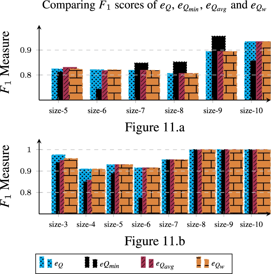
Evaluation in noiseless settings We now re-run the experiments conducted in Section 7 using all metrics, namely ${\mathit{e}}_{\mathit{Q}}$ , ${\mathit{e}}_{{\mathit{Q}}_{min}}$ , ${\mathit{e}}_{{\mathit{Q}}_{\mathrm{avg}}}$ and ${\mathit{e}}_{{\mathit{Q}}_{\mathit{w}}}$ for estimating the quality of clusters of varying sizes: (i) size 5 to 10 for non expert ground truth and (ii) size 3 to 10 for Dutch expert in Fig. 11. The goal of these experiments is to find out which of the metrics performs well overall given the range of cluster sizes. This is done by comparing the metrics respective performances on the basis of their ${\mathit{F}}_1$ measures.

Fig. 11.

Comparative evaluation in noiseless settings by a non expert (11.a) and Dutch domain expert (11.b).

Although in the expert evaluation, ${\mathit{e}}_{{\mathit{Q}}_{min}}$ and ${\mathit{e}}_{{\mathit{Q}}_{\mathrm{avg}}}$ performed equally bad at least once, the observations show that, for both experiments, two main conclusions can be drawn: (1) ${\mathit{e}}_{{\mathit{Q}}_{min}}$ seems unreliable while (2) the rest of the metrics appear to perform alike, giving no solid indication on whether to combine structure and link confidence score.

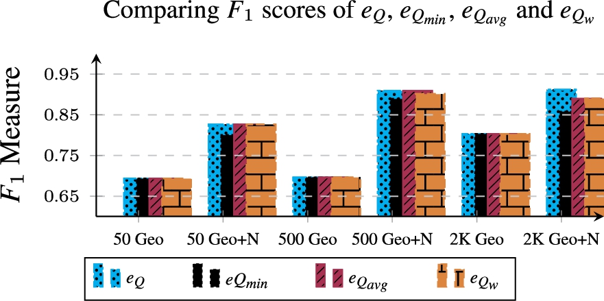
Evaluation in noisy settings Again here, we re-run the same experiments conducted in Section 8 only now using all metrics. This, with the goal of comparing the metrics against each other for further understanding the effect(s) of incorporating the link strength in the structure-based ${\mathit{e}}_{\mathit{Q}}$ metric. Figure 12 again shows no solid evidence for being in favour of structure-based metric or “hybrid-based metrics” (structure + strength). The figure also shows that, whenever the identity network is composed of links with only confidence score of 1 (geo-similarity only), all approaches produce the same estimation score.

Fig. 12.

Comparative evaluation in noisy settings.

Fig. 13.

Evaluation of ${\mathit{e}}_{\mathit{Q}}$ on the ranking from [14].

Evaluation for ranking clustering algorithms Using data from [14], we show in Fig. 13 the results of an experiment where we compare the ranking potential of each approach ( ${\mathit{e}}_{\mathit{Q}}$ , ${\mathit{e}}_{{\mathit{Q}}_{min}}$ , ${\mathit{e}}_{{\mathit{Q}}_{\mathrm{avg}}}$ and ${\mathit{e}}_{{\mathit{Q}}_{\mathit{w}}}$ ) for estimating the quality of an identity network against the algorithm rankings computed by Saeedi et al. (baseline). Bare in mind that here, we not only look at the performance in terms of ${\mathit{F}}_1$ measure but also in terms of ranking capability.

At first, the results show that all approaches appear to rank the algorithms almost equally. However, the deviation in terms of ${\mathit{F}}_1$ score for the ${\mathit{e}}_{{\mathit{Q}}_{min}}$ metric appears quite off compared to the baseline as it shifted considerably below the target’s measures. With ${\mathit{e}}_{{\mathit{Q}}_{\mathrm{avg}}}$ , the previous ${\mathit{F}}_1$ measures move up but not yet close enough to those of the target. In the last option, which implements ${\mathit{e}}_{{\mathit{Q}}_{\mathit{w}}}$ (Equation (10)), the result is comparable to the target ranking and to the ${\mathit{e}}_{\mathit{Q}}$ ranking as well, leading to a first judgement that these two approaches perform better than the other two. According to the visualisation provided by Fig. 13, ${\mathit{e}}_{\mathit{Q}}$ and ${\mathit{e}}_{{\mathit{Q}}_{\mathit{w}}}$ appear to be qualitatively comparable in performance with respect to the ${\mathit{F}}_1$ measures.

With the quantitative comparison provided by Table 8, the ${\mathit{e}}_{\mathit{Q}}$ and ${\mathit{e}}_{{\mathit{Q}}_{\mathit{w}}}$ metrics appear to deviate from the baseline far less on average than the remaining approaches (in 4 cases out of 7 with ties observed in 3 of these cases). This later observation helps breaking the tie between the two metrics ( ${\mathit{e}}_{{\mathit{Q}}_{\mathit{w}}}$ and ${\mathit{e}}_{{\mathit{Q}}_{\mathrm{avg}}}$ ) and indicates that, among hybrid metrics, ${\mathit{e}}_{{\mathit{Q}}_{\mathit{w}}}$ is indeed the way to go. In general, we believe that an hybrid method is potentially better than the original method as it provides additional information that enables us to explain more in details the prediction of the metric and thereby brings the measure closer to expressing “how a network structure can be accurately translated into estimated quality”.

Discussion Although our last experiment seems in general to favour the ${\mathit{e}}_{{\mathit{Q}}_{\mathit{w}}}$ among hybrid metrics, truth is, we need more ground-truth data for making a convincing case on whether one of the hybrids methods is worth the extra computation compared to the original metric, or whether a specific hybrid method works best in some particular settings. For example, we suspect that in settings where matching algorithms are rather permissive, there should be compelling reasons for the link strength to be included. Perhaps, in this situation where link confidence could be assigned a score in the range [0.3, 1] for example, even ${\mathit{e}}_{{\mathit{Q}}_{min}}$ could turn up stable. This, because, in our scenarios, we filter the potentially good links prior to estimating the quality of the network they form. Now, what if this task is given to the metric?

At present, with the limited ground-truth datasets, and relying on the results per matching threshold, the data show that the more precise the matching results get (high threshold), the more the metrics’ predictions converge. For example, at threshold 0.90, all metrics have exactly the same prediction results but the ${\mathit{e}}_{{\mathit{Q}}_{\mathit{w}}}$ metric appears to be the one of choice for thresholds from 0.80 and higher. As the threshold drops to 0.75, ${\mathit{e}}_{{\mathit{Q}}_{\mathrm{avg}}}$ performs better. These observations suggest that the choice of a metric to use depends on the matching algorithms’ precision. In this regard, at very low thresholds, even ${\mathit{e}}_{{\mathit{Q}}_{min}}$ may turn out relevant.

Table 8

Comparing the ranking capability of each of the ${\mathit{e}}_{\mathit{Q}}$ approaches. For each algorithm, we compare the baseline ${\mathit{F}}_1$ scores to those of an ${\mathit{e}}_{\mathit{Q}}$ approach, and only report the difference. Then, for each approach, we compute by how much the ${\mathit{e}}_{\mathit{Q}}$ metric scores under scrutiny deviate on average from those of the baseline. Using the later average, we compare the ${\mathit{e}}_{\mathit{Q}}$ approaches against each other

THRESHOLD	0.75	0.80	0.85	0.90	AVG
CLIP BASELINE	0.9607	0.94908	0.91951	0.72195	0.88781
${\mathit{e}}_{\mathit{Q}}$	0.0107	0.01708	0.03051	0.09595	0.03856
${\mathit{e}}_{{\mathit{Q}}_{min}}$	0.2557	0.24808	0.22351	0.09595	0.20581
${\mathit{e}}_{{\mathit{Q}}_{\mathrm{avg}}}$	0.0317	0.02808	0.03251	0.09595	0.04706
${\mathit{e}}_{{\mathit{Q}}_{\mathit{w}}}$	0.0127	0.01608	0.03051	0.09595	0.03881
CCPIVOT BASELINE	0.75448	0.83596	0.83253	0.62367	0.76166
${\mathit{e}}_{\mathit{Q}}$	0.03852	0.01704	0.00247	0.02967	0.02193
${\mathit{e}}_{{\mathit{Q}}_{min}}$	0.15948	0.19196	0.18053	0.02967	0.14041
${\mathit{e}}_{{\mathit{Q}}_{\mathrm{avg}}}$	0.02852	0.00704	0.00147	0.02967	0.01667
${\mathit{e}}_{{\mathit{Q}}_{\mathit{w}}}$	0.04052	0.01904	0.00247	0.02967	0.02293
CENTER BASELINE	0.85883	0.84593	0.8006	0.54985	0.7638
${\mathit{e}}_{\mathit{Q}}$	0.00683	0.01293	0.0196	0.03285	0.01805
${\mathit{e}}_{{\mathit{Q}}_{min}}$	0.24983	0.23993	0.2096	0.03285	0.18305
${\mathit{e}}_{{\mathit{Q}}_{\mathrm{avg}}}$	0.02283	0.01993	0.0206	0.03285	0.02405
${\mathit{e}}_{{\mathit{Q}}_{\mathit{w}}}$	0.00783	0.01193	0.0196	0.03285	0.01805
CONCOM BASELINE	0.67103	0.80233	0.84734	0.69571	0.7541
${\mathit{e}}_{\mathit{Q}}$	0.02297	0.02167	0.01034	0.08571	0.03517
${\mathit{e}}_{{\mathit{Q}}_{min}}$	0.17103	0.18833	0.19834	0.08571	0.16085
${\mathit{e}}_{{\mathit{Q}}_{\mathrm{avg}}}$	0.00997	0.01067	0.01234	0.08571	0.02967
${\mathit{e}}_{{\mathit{Q}}_{\mathit{w}}}$	0.02297	0.02167	0.01034	0.08571	0.03517
MCENTER BASELINE	0.73774	0.82684	0.84658	0.63994	0.76277
${\mathit{e}}_{\mathit{Q}}$	0.02226	0.01716	0.00558	0.04694	0.02298
${\mathit{e}}_{{\mathit{Q}}_{min}}$	0.18074	0.19284	0.19158	0.04694	0.15302
${\mathit{e}}_{{\mathit{Q}}_{\mathrm{avg}}}$	0.00826	0.00616	0.00758	0.04694	0.01724
${\mathit{e}}_{{\mathit{Q}}_{\mathit{w}}}$	0.02326	0.01716	0.00558	0.04694	0.02323
STAR1 BASELINE	0.72218	0.83963	0.86427	0.70183	0.78198
${\mathit{e}}_{\mathit{Q}}$	0.00782	0.00263	0.02427	0.08983	0.03114
${\mathit{e}}_{{\mathit{Q}}_{min}}$	0.18618	0.21363	0.20927	0.08983	0.17473
${\mathit{e}}_{{\mathit{Q}}_{\mathrm{avg}}}$	0.00618	0.01363	0.02627	0.08983	0.03398
${\mathit{e}}_{{\mathit{Q}}_{\mathit{w}}}$	0.00882	0.00163	0.02427	0.08983	0.03114
STAR2 BASELINE	0.84647	0.8769	0.85674	0.62547	0.80139
${\mathit{e}}_{\mathit{Q}}$	0.00347	0.0069	0.00774	0.01347	0.00789
${\mathit{e}}_{{\mathit{Q}}_{min}}$	0.21147	0.2219	0.19974	0.01347	0.16164
${\mathit{e}}_{{\mathit{Q}}_{\mathrm{avg}}}$	0.02147	0.0179	0.00874	0.01347	0.01539
${\mathit{e}}_{{\mathit{Q}}_{\mathit{w}}}$	0.00247	0.0059	0.00774	0.01347	0.00739

11. Conclusion and future work

11.1. Conclusion

Entity resolution is an essential step in the use of multiple datasets on the semantic web. Since entity resolution algorithms are far from being perfect, the links they discover must often be human validated. Because this is both a costly and an error-prone process, it is desirable to have computer support that can accurately estimate the quality of ilns.

In this paper, we have proposed a metric for precisely this purpose: it estimates the quality of links between entities from multiple datasets, using a combination of graph metrics over the network ( $\mathit{size}\mathrm{>}2$ ) formed by these links. Our metric captures the intuition that high redundancy in such a linking-network correlates with high quality. Furthermore, we have proposed hybrid-metrics that combine structure and link confidence score (strength) for the same purpose of estimating the quality of links between entities. The intuition here is an incremental improvement of the original metric by evaluating the integration of link strength in the quality estimation.

We have tested our metric in three different scenarios. Using a collection of six widely used social science datasets in the first two experimental settings, we compared the predictions of link quality by our metric against human judgements on hundreds of networks involving thousands of links. In both evaluations, our metric correlated strongly with human judgement ( $0.806⩽{\mathit{F}}_1⩽1$ ), and it consistently beats the Majority Class Classifier baseline (except in cases where this is numerically near impossible because of a highly skewed class distribution). In the experimental condition where we deliberately constructed noisy and non-noisy link-networks, we showed that our metric is in general able to exclude poor networks in noisy environments and to include good networks in noise-less environments. With the last experiment, we also show that our metric is able to rank entity resolution algorithms on their quality, using an externally produced dataset and corresponding ground truth. All this amounts to testing the ${\mathit{e}}_{\mathit{Q}}$ metric on a dozen different algorithms and parameter settings.

After showing that our quality metric consistently agrees with human judgement across these different experimental conditions, we re-run all experiments on both the ${\mathit{e}}_{\mathit{Q}}$ and hybrid metrics. The results suggest that the hybrid methods seem to have an effect on estimating the quality of an identity network, only it is yet unclear in what specific condition(s) these metrics bear fruit (do significantly well as opposed to ${\mathit{e}}_{\mathit{Q}}$ ). This yells for more experiments on the matter.

Finally, to encourage replication studies and extensions to our work, all the datasets used in these experiments are available online.

11.2. Future work

Networks of size two The presented metrics are shown to work well in clusters of size bigger than two. Finding ways in which networks of size two can be validated using the ${\mathit{e}}_{\mathit{Q}}$ metrics would be an added value as the amount of clusters of such size is not negligible. The ${\mathit{e}}_{\mathit{Q}}$ metric is about corroborating links using other redundant links. It can be extended by combining it with external knowledge (external to the ILN) for corroborating an existing link. For example, if we use a relation like “marriage” as external knowledge to interconnect ILNs, such information can then be used to corroborate pair of nodes. Hence, if there exist two records A and B reporting the marriage of John and Mary then the pair $⟨\mathit{Joh}{\mathit{n}}_{\mathit{A}}\mathrm{,}\mathit{Joh}{\mathit{n}}_{\mathit{B}}⟩$ can be corroborated by the pair $⟨\mathit{Mar}{\mathit{y}}_{\mathit{A}}\mathrm{,}\mathit{Mar}{\mathit{y}}_{\mathit{B}}⟩$ and vice-versa.

In this context, when a link is corroborated with the use of external knowledge, then the metric can be applied to networks lacking redundant identity-links such as networks of size two. In addition, such modification may improve the ${\mathit{e}}_{\mathit{Q}}$ prediction on the quality of incomplete networks such as those in a star or line topology. We, furthermore expect some external knowledge to be useful for detecting inconsistency in links between resources in a candidate identity network. For example, John cannot be his own father. In this scenario, the knowledge could then be used to immediately flag a network as bad.

Dynamic link adjustment The current work ideally takes clustered ilns as input. However, when such networks are not provided, it simply takes the output of an entity resolution algorithm as given, applies the simple clustering algorithm (Algorithm 1) and tries to estimate the quality of that output. A closer coupling between our metric and an entity resolution algorithm would allow this algorithm to dynamically adjust its output based on the ${\mathit{e}}_{\mathit{Q}}$ quality estimates. Similarly, embedded in a user-interface, the score of our metric could help the user to give the final judgement to accept or reject an iln.

Parameter tuning In this work, we qualitatively determined the sigmoid hyper-parameter (1.6), the discrete ${\mathit{e}}_{\mathit{Q}}$ intervals and the string similarity thresholds. Our experiments show that these chosen values are sufficient to get good results in multiple experiments, but we do not claim them to be optimal. Experimenting on fine-tuning these parameters using the current ground-truth and data from other domains would help understanding how and when different choices could lead to an increase or a decrease of the metrics’ predictive power. Also, experimenting on whether one or more metrics (bridge, diameter and closure) can be left out or whether to always use the sigmoid penalty can further help strengthen our intuition that high redundancy correlates with high quality.