VIG: Data scaling for OBDA benchmarks

Abstract

In this paper we describe vig, a data scaler for Ontology-Based Data Access (OBDA) benchmarks. Data scaling is a relatively recent approach, proposed in the database community, that allows for quickly scaling an input data instance to s times its size, while preserving certain application-specific characteristics. The advantages of the scaling approach are that the same generator is general, in the sense that it can be re-used on different database schemas, and that users are not required to manually input the data characteristics. In the vig system, we lift the scaling approach from the pure database level to the OBDA level, where the domain information of ontologies and mappings has to be taken into account as well. vig is efficient and notably each tuple is generated in constant time. To evaluate vig, we have carried out an extensive set of experiments with three datasets (BSBM, DBLP, and NPD), using two OBDA systems (Ontop and D2RQ), backed by two relational database engines (MySQL and PostgreSQL), and compared with real-world data, ad-hoc data generators, and random data generators. The encouraging results show that the data scaling performed by vig is efficient and that the scaled data are suitable for benchmarking OBDA systems.

1. Introduction

An important research problem in Big Data is how to provide end-users with transparent access to the data, abstracting from storage details. The paradigm of Ontology-based Data Access (OBDA) [7,27] provides an answer to this problem that is very close to the spirit of the Semantic Web. In OBDA, the data stored in a relational database is presented to the end-users as a virtual RDF graph, whose vocabulary is provided by the classes and properties of an ontology, over which SPARQL queries can be posed. This solution is realized through mappings that establish a link between the ontology and the database, by specifying how to instantiate the classes and properties in the ontology by means of queries over the database.

A lot of research on optimization techniques for OBDA has been carried out recently, with the aim of making this paradigm effective in practice [4,5,11,15,19,23,28]. In order to evaluate the effectiveness of optimizations, some benchmarks have been proposed and applied to the OBDA setting.1

¹

http://dl.kr.org/omqbench/

However, proper benchmarking of OBDA systems requires scalability analyses taking into account data instances of increasing volume. Such instances are often provided by generators of synthetic data. However, such generators are either complex ad-hoc implementations working for a specific schema, or require considerable manual input by the end-user. The latter problem is exacerbated in the OBDA setting, where database schemas tend to be particularly big and complex (e.g., 70 tables, some with more than 80 columns in the NPD benchmark [17]). This contributes to the slow creation of new benchmarks, and the same old benchmarks become more and more misused over a long period of time. For instance, evaluations on OBDA systems are usually performed on benchmarks originally designed for triple stores, although these two types of systems are substantially different and present different challenges [17].

Data scaling [26] is a recent approach that tries to overcome this problem by automatically tuning the generation parameters through statistics collected over an initial data instance. Hence, the same generator can be reused in different contexts, as long as an initial data instance is available. A measure of quality for the produced data is defined in terms of results for the available queries, which should be similar to the ones observed for real data of comparable volume.

In the context of OBDA, however, taking as the only parameter for generation an initial data instance does not produce data of acceptable quality, since the generated data has to comply with constraints deriving from the structure of the mappings and the ontology, which in turn derive from the application domain.

In this work we present the vig system, a data scaler for OBDA benchmarks that addresses these issues. In vig, the scaling approach is lifted from the instance level to the OBDA level, where the domain information of ontologies and mappings has to be taken into account as well. vig is very efficient and suitable to generate huge amounts of data, as tuples are generated in constant time without disk accesses or need to retrieve previously generated values. Furthermore, different instances of vig can be delegated to different machines, and parallelization can scale up to the number of columns in the schema, without communication overhead. Finally, vig produces data in the form of csv files that can be imported easily by any relational database system.

To evaluate vig, we have carried out an extensive set of experiments with three datasets (BSBM, DBLP, and NPD) resembling information needs in real-world use cases, using two OBDA systems (Ontop and D2RQ), backed by two relational database engines (MySQL and PostgreSQL), and compared with real-world data, ad-hoc data generators, and random data generators. In numbers, we ran in total 8042 queries over 49 database instances, among which 4 (DBLP and NPD under MySQL and PostgreSQL) are real-world data, 3 are original synthetic data (MySQL and PostgreSQL) from BSBM, and the rest are generated by vig in different modes. The results over the three datasets are encouraging and show that the data scaling performed by vig is efficient and that the scaled data are suitable for benchmarking OBDA systems. Moreover, the results obtained over the NPD dataset demonstrate the benefits of taking into account mappings in the generation of data.

The rest of the paper is structured as follows. In Section 2, we introduce the basic notions and notation to understand this paper. In Section 3, we define the scaling problem and discuss important measures on the produced data that define the quality of instances in a given OBDA setting. In Section 4, we discuss the vig algorithm, and how it ensures that data conforming to the identified measures is produced. In Section 5, we provide an empirical evaluation of vig, in terms of both resource consumption and quality of produced data, and in Section 6.1 we discuss the impact of multi-attribute foreign keys on the generation process. Sections 7 and 8 contain related work and conclusions, respectively.

This paper is a revised and significantly extended version of an article containing preliminary results that was presented at the Workshop on Benchmarking Linked Data (BLINK) 2016 [18].2

²

With respect to [18], apart from providing many more details on the vig algorithm, we have also carried out more extensive experiments, by including DBLP as a third dataset (cf. Section 5.3), by using as OBDA system also D2RQ, in addition to Ontop, and by relying on PostgreSQL, in addition to MySQL, as relational database engine (cf. Section 5.1).

2. Basic notions and notation

We assume that the reader has moderate knowledge of OBDA, and refer for it to the abundant literature on the subject, like [6]. Moreover, we assume familiarity with basic notions from probability calculus and statistics.

Table 1

Portion of the ontology for the NPD benchmark. The first three axioms (left to right) state that the classes Exploration Wellbore ( $\mathsf{ExpWellbore}$ ), Shallow Wellbore ( $\mathsf{ShWellbore}$ ), and Suspended Wellbore ( $\mathsf{SuspWellbore}$ ) are subclasses of the class $\mathsf{Wellbore}$ . The fourth axiom states that the classes $\mathsf{ExpWellbore}$ and $\mathsf{ShWellbore}$ are disjoint

$\begin{array}{ccc}\hfill \mathsf{ExpWellbore}& \hfill ⊑\hfill & \mathsf{Wellbore}\hfill \\ \hfill \mathsf{ShWellbore}& \hfill ⊑\hfill & \mathsf{Wellbore}\hfill \\ \hfill \mathsf{SuspWellbore}& \hfill ⊑\hfill & \mathsf{Wellbore}\hfill \\ \hfill \mathsf{ExpWellbore}\sqcap \mathsf{ShWellbore}& \hfill ⊑\hfill & \perp \hfill \end{array}$

The W3C standard ontology language for OBDA is OWL 2 QL [20]. For the sake of conciseness, we consider here its mathematical underpinning ${\mathit{\text{DL-Lite}}}_{\mathcal{R}}$ [8]. Table 1 shows a portion of the ${\mathit{\text{DL-Lite}}}_{\mathcal{R}}$ ontology from the NPD benchmark, which is the foundation block of our running example.

Table 2

Queries for our running example

$\begin{array}{cc}{\mathit{q}}_1\mathrm{(}\mathit{y}\mathrm{)}\hfill & \leftarrow \mathsf{Wellbore}\mathrm{(}\mathit{y}\mathrm{)}\mathrm{,}\mathsf{shWellboreForField}\mathrm{(}\mathit{x}\mathrm{,}\mathit{y}\mathrm{)}\hfill \\ {\mathit{q}}_2\mathrm{(}\mathit{x}\mathrm{,}\mathit{n}\mathrm{,}\mathit{y}\mathrm{)}\hfill & \leftarrow \mathsf{Wellbore}\mathrm{(}\mathit{x}\mathrm{)}\mathrm{,}\mathsf{name}\mathrm{(}\mathit{x}\mathrm{,}\mathit{n}\mathrm{)}\mathrm{,}\mathsf{complYear}\mathrm{(}\mathit{x}\mathrm{,}\mathit{y}\mathrm{)}\hfill \end{array}$

Table 3

Mappings from the NPD benchmark

$\begin{array}{ccc}\mathsf{ExpWellbore}\mathrm{(}\mathit{w}\mathrm{(}\mathtt{\text{id}}\mathrm{)}\mathrm{)}\hfill & \hfill ⇝\hfill & \mathtt{\text{exploration\_wellbores(id,active,name,year)}}\hfill \\ \mathsf{ShWellbore}\mathrm{(}\mathit{w}\mathrm{(}\mathtt{\text{id}}\mathrm{)}\mathrm{)}\hfill & \hfill ⇝\hfill & \mathtt{\text{shallow\_wellbores(id,name,year,fid)}}\hfill \\ \mathsf{SuspWellbore}\mathrm{(}\mathit{w}\mathrm{(}\mathtt{\text{id}}\mathrm{)}\mathrm{)}\hfill & \hfill ⇝\hfill & \mathtt{\text{exploration\_wellbores(id,active,name,year), active=’false’}}\hfill \\ \mathsf{Field}\mathrm{(}\mathit{f}\mathrm{(}\mathtt{\text{fid}}\mathrm{)}\mathrm{)}\hfill & \hfill ⇝\hfill & \mathtt{\text{fields(fid,name)}}\hfill \\ \mathsf{complYear}\mathrm{(}\mathit{w}\mathrm{(}\mathtt{\text{id}}\mathrm{)}\mathrm{,}\mathtt{\text{year}}\mathrm{)}\hfill & \hfill ⇝\hfill & \mathtt{\text{exploration\_wellbores(id,active,name,year)}}\hfill \\ \mathsf{complYear}\mathrm{(}\mathit{w}\mathrm{(}\mathtt{\text{id}}\mathrm{)}\mathrm{,}\mathtt{\text{year}}\mathrm{)}\hfill & \hfill ⇝\hfill & \mathtt{\text{shallow\_wellbores(id,name,year,fid)}}\hfill \\ \mathsf{name}\mathrm{(}\mathit{w}\mathrm{(}\mathtt{\text{id}}\mathrm{)}\mathrm{,}\mathtt{\text{name}}\mathrm{)}\hfill & \hfill ⇝\hfill & \mathtt{\text{exploration\_wellbores(id,active,name,year)}}\hfill \\ \mathsf{name}\mathrm{(}\mathit{w}\mathrm{(}\mathtt{\text{id}}\mathrm{)}\mathrm{,}\mathtt{\text{name}}\mathrm{)}\hfill & \hfill ⇝\hfill & \mathtt{\text{shallow\_wellbores(id,name,year,fid)}}\hfill \\ \mathsf{shWellboreForField}\mathrm{(}\mathit{w}\mathrm{(}\mathtt{\text{id}}\mathrm{)}\mathrm{,}\mathit{f}\mathrm{(}\mathtt{\text{fid}}\mathrm{)}\mathrm{)}\hfill & \hfill ⇝\hfill & \mathtt{\text{shallow\_wellbores(id,name,year,fid), fields(fid,fname)}}\hfill \end{array}$

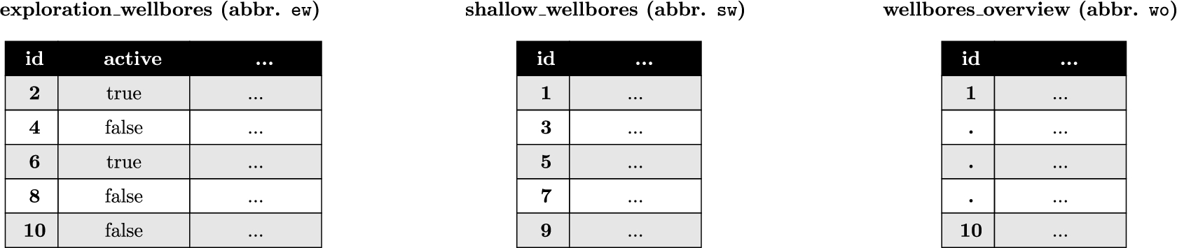
Results from the evaluation of the queries on the source part build assertions in the ontology. For example, each tuple $\mathrm{(}\mathit{a}\mathrm{,}\mathit{b}\mathrm{,}\mathit{c}\mathrm{,}\mathit{d}\mathrm{)}$ in a relation for shallow_wellbores generates an object $\mathit{w}\mathrm{(}\mathit{a}\mathrm{)}$ and an assertion $\mathsf{ShWellbore}\mathrm{(}\mathit{w}\mathrm{(}\mathit{a}\mathrm{)}\mathrm{)}$ in the ontology. In the R2RML mappings for the original NPD benchmark the term $\mathit{w}\mathrm{(}\mathtt{\text{id}}\mathrm{)}$ corresponds to the URI template npd:wellbore/{id}. Columns named id are primary keys, and the column fid in shallow_wellbores is a foreign key for the primary key fid of the table fields.

The W3C standard query language in OBDA is SPARQL [14], with queries evaluated under the OWL 2 QL entailment regime [16]. Intuitively, under these semantics each basic graph pattern (BGP) can be seen as a single conjunctive query (CQ) without existentially quantified variables. As in our examples we only refer to SPARQL queries containing exactly one BGP, we use the more concise syntax for CQs rather than the SPARQL syntax. Table 2 shows the two queries used in our running example.

The mapping component links predicates in the ontology to queries over the underlying relational database. To present our techniques, we need to introduce this component in a formal way. The standard W3C language for mappings is R2RML [10], however here we use a more concise syntax that is common in the OBDA literature. Formally, a mapping assertion $\mathfrak{m}$ is an expression of the form $\mathit{X}\mathrm{(}\overrightarrow{\mathit{f}}\mathrm{,}\overrightarrow{\mathit{x}}\mathrm{)}⇝conj\mathrm{(}\overrightarrow{\mathit{y}}\mathrm{)}$ , consisting of a source part $conj\mathrm{(}\overrightarrow{\mathit{y}}\mathrm{)}$ , which is a CQ whose output variables are $\overrightarrow{\mathit{y}}$ , and a target part $\mathit{X}\mathrm{(}\overrightarrow{\mathit{f}}\mathrm{,}\overrightarrow{\mathit{x}}\mathrm{)}$ , which is an atom whose predicate is X over terms (also called templates) built using function symbols $\overrightarrow{\mathit{f}}$ and variables $\overrightarrow{\mathit{x}}\subseteq \overrightarrow{\mathit{y}}$ . We say that such a mapping $\mathfrak{m}$ defines the predicate X. A basic mapping is a mapping whose source part is a query containing exactly one atom. Table 3 shows the mappings for our running example, and provides a short description of how these mappings are used in order to create a (virtual) set of assertions.

For the rest of the paper we fix an OBDA instance $\mathrm{(}\mathcal{T}\mathrm{,}\mathit{M}\mathrm{,}\mathrm{\Sigma }\mathrm{,}\mathcal{D}\mathrm{)}$ , where $\mathcal{T}$ is an OWL 2 QL ontology, Σ is a database schema with foreign and primary key dependencies, $\mathcal{M}$ is a set of mappings linking predicates in $\mathcal{T}$ to queries over Σ, and $\mathcal{D}$ is a database instance that satisfies the dependencies in Σ and such that the assertions created from $\mathcal{D}$ via mappings $\mathcal{M}$ do not violate the disjointness axioms in $\mathcal{T}$ . We denote by $col\mathrm{(}\mathrm{\Sigma }\mathrm{)}$ the set of all columns in Σ. Given a column $\mathit{C}\in col\mathrm{(}\mathrm{\Sigma }\mathrm{)}$ , we denote by ${\mathit{C}}^{\mathcal{D}}$ the set of values for C in $\mathcal{D}$ . Finally, given a term $\mathit{f}\mathrm{(}\overrightarrow{\mathit{x}}\mathrm{)}$ , where $\overrightarrow{\mathit{x}}=\mathrm{(}{\mathit{x}}_1\mathrm{,}\dots \mathrm{,}{\mathit{x}}_{\mathit{p}}\mathrm{,}\dots \mathrm{,}{\mathit{x}}_{\mathit{n}}\mathrm{)}$ , we denote the argument ${\mathit{x}}_{\mathit{p}}$ at position p by $\mathit{f}\mathrm{(}\overrightarrow{\mathit{x}}\mathrm{)}{|}_{\mathit{p}}$ .

3. Data scaling for OBDA benchmarks: The vig approach

The data scaling problem introduced in [26] is formulated as follows:

Definition 3.1 (Data Scaling Problem).

Given a database instance $\mathcal{D}$ for a schema Σ, and a scale factor s, produce a database instance ${\mathcal{D}}^{\prime }$ for Σ which is similar to $\mathcal{D}$ but s times its size.

The notion of similarity is application-based. Being our goal benchmarking, we define similarity in terms of execution times for the evaluation of the queries in the benchmark. More precisely, consider a (real world) database instance ${\mathcal{D}}_0$ and a larger (real world) instance ${\mathcal{D}}_1$ into which ${\mathcal{D}}_0$ has evolved over time. Consider also an instance ${\mathcal{D}}_0^{\prime }$ scaled from ${\mathcal{D}}_0$ up to a size comparable to that of ${\mathcal{D}}_1$ . Then, the measured execution times for the evaluation of the benchmark queries over ${\mathcal{D}}_0^{\prime }$ should be close to the measured execution times for the evaluation of the same queries over ${\mathcal{D}}_1$ . In [26], the authors do not consider benchmark queries to be available to the generator, since their goal is broader than benchmarking over a pre-defined set of queries. In OBDA benchmarking, however, the (SQL) workload for the database can be estimated from the mapping component. Therefore, vig includes the mappings in the analysis, so as to obtain a more realistic and OBDA-tuned generation.

Concerning the size, similarly to other approaches, vig scales each table in $\mathcal{D}$ by a factor of s.

3.1. Similarity measures for OBDA and their rationale

Our notion of similarity is an ideal one, but also an abstract one, as it does not provide any guideline on how the data should be generated. In this section we overview the concrete similarity measures which are used by vig to guide the generation process. Our idea is that generating instances similar to the initial one with respect to these concrete measures can be a suitable way to produce instances that are similar also with respect to our ideal abstract similarity measure.

Schema dependencies The scaled instance ${\mathcal{D}}^{\prime }$ should be a valid instance for Σ. vig is, to the best of our knowledge, the only data scaler able to generate in constant time tuples that satisfy multi-attribute primary keys for weakly-identified entities.3

³

In a relational database, a weak entity is an entity that cannot be uniquely identified by its attributes alone.

The current algorithm of vig supports single-attribute foreign keys, but not yet multi-attribute foreign keys. We refer to Section 6.1 for a discussion on the impact of multi-attribute foreign keys on the generation process.

Column-based duplicates and NULL ratios These two parameters, which respectively measure the ratio of duplicates and of NULLs in a given column, are commonly used for the cost estimation performed by query planners in databases. By default, vig maintains them in ${\mathcal{D}}^{\prime }$ to preserve the cost of a number of algebra operations, such as projections or joins between columns in a key-foreign key relationship (e.g., the join from the last mapping in our running example). This default behavior, however, is not applied with fixed-domain columns, which are columns whose content does not depend on the size of the database instance. An example of fixed-domain column is the column active in the table exploration_wellbore, because depending on the value of active, the elements of id are partitioned into a fixed number of types, corresponding to classes in the ontology.4

⁴

The number of classes in the ontology does not depend on the size of the data instance.

vig analyzes the mappings to detect such cases of fixed-domain columns, and additional fixed-domain columns can be manually specified by the user. To generate values for a fixed-domain column, vig reuses the values found in $\mathcal{D}$ so as to prevent empty answers for the SQL queries in the mappings. For instance, a value ‘false’ must be generated for the column active in order to produce objects for the class $\mathsf{SuspWellbore}$ .

Fig. 1.

The VIG algorithm.

vig generates values in columns according to a uniform distribution, that is, all values in a column have the same probability of being repeated. Replication of the distributions from $\mathcal{D}$ will be included in a future release of vig.

Size of columns clusters, and disjointness Query ${\mathit{q}}_1$ from our running example returns an empty set of answers, regardless of the considered data instance. This is because ${\mathit{q}}_1$ performs a join between wellbores and fields, but the function w used to build objects for the class $\mathsf{Wellbore}$ does not match with the function f used to build objects for the class $\mathsf{Field}$ . Indeed, fields and wellbores are two different entities and a join between them is meaningless.

On the other hand, a standard OBDA translation of ${\mathit{q}}_2$ into SQL produces a union of CQs, in which several of these CQs contain joins between the tables exploration_wellbores and shallow_wellbores. This is possible only because the mappings for $\mathsf{Wellbore}$ , $\mathsf{name}$ , and $\mathsf{complYear}$ all use the same unary function symbol w to define wellbores. Intuitively, every pair of terms over the same function symbol and appearing in the target of two distinct basic mappings identifies sets of columns for which the join operation is semantically meaningful.5

⁵

Therefore, between such identified sets of columns a join could occur during the evaluation of a user query.

Generating data that guarantees the correct cost for these joins is crucial in order to deliver a realistic evaluation. In our example, a join between exploration_wellbores and shallow_wellbores over the attribute id is empty under $\mathcal{D}$ (in fact, $\mathsf{ExpWellbore}$ and $\mathsf{ShWellbore}$ are disjoint classes, and by assumption $\mathcal{D}$ respects the disjointness constraints of the ontology). vig is able to replicate this fact in  ${\mathcal{D}}^{\prime }$ . This implies that vig can generate data satisfying disjointness constraints declared over classes whose individuals are constructed from a unary template in a basic mapping, if $\mathcal{D}$ satisfies those constraints.

4. The vig algorithm

In this section we show how vig realizes the measures described in the previous section. To allow the reader to concentrate on the important aspects, and considering that different database systems use different names for datatypes, we do not discuss low-level details, e.g., which domains for attributes are acceptable. We provide such details in the online resource6

⁶

https://ontop.github.io/vig/

where the generator is made available.

Algorithm 1 shows a high-level view of vig. Each comment in the code refers to a specific paragraph name in this section, where the respective code is explained and discussed. The function names in the pseudo-code recall the actual method names of the vig implementation, which is freely available on GitHub7

⁷

https://github.com/ontop/vig

and open to contributions.

At the high-level, the vig algorithm consists of two phases: the analysis phase, and the generation phase. In the analysis phase, the input data instance $\mathcal{D}$ is analyzed to collect statistics and create a set $ints\mathrm{(}\mathit{C}\mathrm{)}$ of intervals associated to each column C in the database schema. Each interval $\mathit{I}\in ints\mathrm{(}\mathit{C}\mathrm{)}$ for a column C is a structure $[min\mathrm{,}max]$ keeping track of a minimum and maximum integer index. In the generation phase, a pseudo random number generator is used to randomly choose indexes from each of these intervals. Then, for each column C, an injective function ${\mathit{g}}_{\mathit{C}}$ is applied to transform each chosen index $\mathit{i}\in \mathit{I}$ , $\mathit{I}\in ints\mathrm{(}\mathit{C}\mathrm{)}$ , into a database value according to the datatype of C.

From now on, let s be a scale factor, and let $dist\mathrm{(}\mathit{C}\mathrm{,}\mathcal{D}\mathrm{)}$ denote the number of distinct non-NULL values in a column C in the database instance $\mathcal{D}$ . Let $size\mathrm{(}\mathit{T}\mathrm{,}\mathcal{D}\mathrm{)}$ denote the number of tuples occurring in the table T in the database instance $\mathcal{D}$ . To illustrate the algorithm, we consider a source instance $\mathcal{D}$ that contains values as shown in Fig. 2, and a scaling factor $\mathit{s}=2$ .

Fig. 2.

Input data instance $\mathcal{D}$ . Columns id from tables exploration_wellbores and shallow_wellbores are foreign keys of column id from table wellbores_overview.

4.1. Analysis phase

The goal of this phase is to create intervals of indexes for each column that will be used as an input to the generation phase. These intervals are created while satisfying certain constraints over the database schema, mappings, and statistical information on the source database. The analysis phase consists of the following 5 stages:

1. initialization: reading of the database schema and statistics over the source database;

2. creation of intervals: creation, starting from the statistics, of initial intervals of indexes to associate to each column;

3. satisfaction of primary keys: ensuring that primary key constraints are satisfied in the scaled instance by adapting the intervals boundaries;

4. columns cluster analysis: identification of semantically related columns through schema and mappings analysis, and adaptation of the intervals boundaries;

5. satisfaction of foreign keys: ensuring that foreign key constraints are satisfied in the scaled instance by adapting the intervals boundaries.

We now detail each of these stages.

Initialization For each table T, vig sets the number $size\mathrm{(}\mathit{T}\mathrm{,}{\mathcal{D}}^{\prime }\mathrm{)}$ of tuples to generate to $\mathit{s}·size\mathrm{(}\mathit{T}\mathrm{,}\mathcal{D}\mathrm{)}$ . Then, vig calculates the number of distinct non-NULL values that need to be generated for each column, given s and $\mathcal{D}$ . That is, for each column C, if C is not fixed-domain then vig sets $dist\mathrm{(}\mathit{C}\mathrm{,}{\mathcal{D}}^{\prime }\mathrm{)}:=\mathit{s}·dist\mathrm{(}\mathit{C}\mathrm{,}\mathcal{D}\mathrm{)}$ . Otherwise, $dist\mathrm{(}\mathit{C}\mathrm{,}{\mathcal{D}}^{\prime }\mathrm{)}$ is set to $dist\mathrm{(}\mathit{C}\mathrm{,}\mathcal{D}\mathrm{)}$ . To determine whether a column is fixed-domain, vig searches in $\mathcal{M}$ for mappings of shape $$\begin{array}{c}\mathit{A}\mathrm{(}\mathit{f}\mathrm{(}\overrightarrow{\mathit{a}}\mathrm{)}\mathrm{)}⇝\mathit{T}\mathrm{(}\overrightarrow{\mathit{b}}\mathrm{)}\mathrm{,}{\mathit{b}}_1={\mathit{c}}_1\mathrm{,}\dots \mathrm{,}{\mathit{b}}_{\mathit{n}}={\mathit{c}}_{\mathit{n}}\end{array}$$ where A is a class, T is a table, ${\mathit{c}}_1\mathrm{,}\dots \mathrm{,}{\mathit{c}}_{\mathit{n}}$ are constants, and ${\mathit{b}}_1\mathrm{,}\dots \mathrm{,}{\mathit{b}}_{\mathit{n}}$ are columns in $\overrightarrow{\mathit{b}}$ . For each such mapping, vig marks the columns ${\mathit{b}}_1\mathrm{,}\dots \mathrm{,}{\mathit{b}}_{\mathit{n}}$ as fixed-domain.

Example 4.1.

For the tables in Fig. 2, vig sets $size\mathrm{(}\mathtt{\text{ew}}\mathrm{,}{\mathcal{D}}^{\prime }\mathrm{)}=size\mathrm{(}\mathtt{\text{sw}}\mathrm{,}{\mathcal{D}}^{\prime }\mathrm{)}=2·5=10$ , and $size\mathrm{(}\mathtt{\text{wo}}\mathrm{,}{\mathcal{D}}^{\prime }\mathrm{)}=2·10=20$ . Values for statistics $dist\mathrm{(}\mathit{T}.\mathtt{\text{id}}\mathrm{,}{\mathcal{D}}^{\prime }\mathrm{)}$ , where T is one of $\{\mathtt{\text{ew}}\mathrm{,}\mathtt{\text{sw}}\mathrm{,}\mathtt{\text{wo}}\}$ , are set in the same way, because the id columns do not contain duplicate values. The column ew.active is marked as fixed-domain, because of the third mapping in Table 3. Therefore, vig sets $dist\mathrm{(}\mathtt{\text{ew}}.\mathtt{\text{active}}\mathrm{)}=2$ .

Creation of intervals When C is a numerical column, vig initializes $ints\mathrm{(}\mathit{C}\mathrm{)}$ to the interval ${\mathit{I}}_{\mathit{C}}:=[min\mathrm{(}\mathit{C}\mathrm{,}\mathcal{D}\mathrm{)}\mathrm{,}min\mathrm{(}\mathit{C}\mathrm{,}\mathcal{D}\mathrm{)}+dist\mathrm{(}\mathit{C}\mathrm{,}{\mathcal{D}}^{\prime }\mathrm{)}-1]$ of distinct values to be generated, where $min\mathrm{(}\mathit{C}\mathrm{,}\mathcal{D}\mathrm{)}$ denotes the minimum value occurring in ${\mathit{C}}^{\mathcal{D}}$ . Otherwise, if C is non-numerical, $ints\mathrm{(}\mathit{C}\mathrm{)}$ is initialized to the interval ${\mathit{I}}_{\mathit{C}}:=[1\mathrm{,}dist\mathrm{(}\mathit{C}\mathrm{,}{\mathcal{D}}^{\prime }\mathrm{)}]$ . We recall that the elements in the intervals in $ints\mathrm{(}\mathit{C}\mathrm{)}$ are transformed into values of the desired datatype by a suitable injective function in the final generation step.

Example 4.2.

Following on our running example, vig creates in this phase the intervals ${\mathit{I}}_{\mathtt{\text{ew.id}}}=[2\mathrm{,}11]$ , ${\mathit{I}}_{\mathtt{\text{ew.active}}}=[1\mathrm{,}2]$ , ${\mathit{I}}_{\mathtt{\text{sw.id}}}=[1\mathrm{,}10]$ , and ${\mathit{I}}_{\mathtt{\text{wo.id}}}=[1\mathrm{,}20]$ . Then, the intervals are associated to the respective columns. Namely, $ints\mathrm{(}\mathtt{\text{ew.id}}\mathrm{)}=\{{\mathit{I}}_{\mathtt{\text{ew.id}}}\}$ , … , $ints\mathrm{(}\mathtt{\text{wo.id}}\mathrm{)}=\{{\mathit{I}}_{\mathtt{\text{wo.id}}}\}$ .

Satisfaction of primary keys The generation of distinct tuples depends on the pseudo-random number generator adopted. Formally, a pseudo-random number generator is a sequence of integers ${\mathrm{(}{\mathit{s}}_{\mathit{i}}\mathrm{)}}_{\mathit{i}\in \mathbb{N}}$ defined through a transition function ${\mathit{s}}_{\mathit{k}}:=\mathit{f}\mathrm{(}{\mathit{s}}_{\mathit{k}-1}\mathrm{)}$ . vig adopts a particular class of pseudo-random generators, introduced in [13], and based on multiplicative groups modulo a prime number. Such generators are able to generate a permutation of the indexes in an interval. In formal terms, let n be the number of distinct values to generate, and let g be a generator for the multiplicative group modulo a prime number p, with $\mathit{p}\mathrm{>}\mathit{n}$ . Consider the sequence $\mathit{S}:=⟨{\mathit{g}}^{\mathit{i}}\mathit{\text{mod }}\mathit{p}|\mathit{i}=1\mathrm{,}\dots \mathrm{,}\mathit{p}\text{ and }\mathrm{(}{\mathit{g}}^{\mathit{i}}\mathit{\text{mod }}\mathit{p}\mathrm{)}⩽\mathit{n}⟩$ . Then S is a permutation of values in the interval $[1\mathrm{,}\dots \mathrm{,}\mathit{n}]$ .

We now explain how such number generator can be used to generate tuples of values satisfying the primary key constraints in the schema. Let $\mathit{K}=\{{\mathit{C}}_1\mathrm{,}\dots \mathrm{,}{\mathit{C}}_{\mathit{n}}\}$ be the primary key of a table T. In order to ensure that values generated for each column through our pseudo-random generator do not lead to tuples with duplicate values for the key K, it suffices that the least common multiple $lcm\mathrm{(}dist\mathrm{(}{\mathit{C}}_1\mathrm{,}{\mathcal{D}}^{\prime }\mathrm{)}\mathrm{,}\dots \mathrm{,}dist\mathrm{(}{\mathit{C}}_{\mathit{n}}\mathrm{,}{\mathcal{D}}^{\prime }\mathrm{)}\mathrm{)}$ of the number of distinct values to generate in each column is greater than the number $tuples\mathrm{(}\mathit{T}\mathrm{,}{\mathcal{D}}^{\prime }\mathrm{)}$ of tuples to generate for the table T. While this condition is not satisfied, vig increases by 1 $dist\mathrm{(}{\mathit{C}}_{\mathit{i}}\mathrm{,}{\mathcal{D}}^{\prime }\mathrm{)}$ for a suitably chosen column ${\mathit{C}}_{\mathit{i}}$ in K. Observe that the only side effect of this is a small deviation on the number of distinct values to generate for a column. Once the condition holds, data can be generated independently for each column without risk of generating duplicate tuples for K.

Columns cluster analysis In this phase, vig analyzes $\mathcal{M}$ in order to identify columns that could be joined in a translation to SQL, and groups them together into pre-clusters. Formally, let ${\mathit{X}}_1\mathrm{(}\overrightarrow{{\mathit{f}}_1}\mathrm{,}\overrightarrow{{\mathit{x}}_1}\mathrm{)}\mathrm{,}\dots$ , ${\mathit{X}}_{\mathit{m}}\mathrm{(}\overrightarrow{{\mathit{f}}_{\mathit{m}}}\mathrm{,}\overrightarrow{{\mathit{x}}_{\mathit{m}}}\mathrm{)}$ be the atoms defined by basic mappings in $\mathcal{M}$ , where variables correspond to qualified column names.8

⁸

A qualified column name is a string of the form T.C, where T is a table name and C a column name.

Consider the set $\mathcal{F}={\bigcup }_{\mathit{i}=1\dots \mathit{m}}\{\mathit{f}\mathrm{(}\overrightarrow{\mathit{x}}\mathrm{)}\mid \mathit{f}\mathrm{(}\overrightarrow{\mathit{x}}\mathrm{)}\text{ is a term in }{\mathit{X}}_{\mathit{i}}\mathrm{(}\overrightarrow{{\mathit{f}}_{\mathit{i}}}\mathrm{,}\overrightarrow{{\mathit{x}}_{\mathit{i}}}\mathrm{)}\}$ of all the terms occurring in such atoms. For each function f and valid position p in f, we define a pre-cluster ${\mathfrak{pc}}_{\mathit{f}{|}_{\mathit{p}}}$ as the set of columns ${\mathfrak{pc}}_{\mathit{f}{|}_{\mathit{p}}}=\{\mathit{f}\mathrm{(}\overrightarrow{\mathit{x}}\mathrm{)}{|}_{\mathit{p}}\mid \mathit{f}\mathrm{(}\overrightarrow{\mathit{x}}\mathrm{)}\in \mathcal{F}\}$ .

Example 4.3.

For our running example, we have $$\begin{array}{rcl}\mathcal{F}& =& \{\mathit{w}\mathrm{(}\mathtt{\text{ew.id}}\mathrm{)}\mathrm{,}\mathit{w}\mathrm{(}\mathtt{\text{sw.id}}\mathrm{)}\mathrm{,}\\ & & \mathit{f}\mathrm{(}\mathtt{\text{fields.fid}}\mathrm{)}\}.\end{array}$$ There are two pre-clusters, namely ${\mathfrak{pc}}_{\mathit{w}{|}_1}=\{\mathtt{\text{ew.id}}\mathrm{,}\mathtt{\text{sw.id}}\}$ and ${\mathfrak{pc}}_{\mathit{f}{|}_1}=\{\mathtt{\text{fields.fid}}\}$ .

vig evaluates on $\mathcal{D}$ all combinations of joins between columns in a pre-cluster $\mathfrak{pc}$ , and produces values in ${\mathcal{D}}^{\prime }$ so that the selectivities for these joins are maintained. In order to do so, the intervals for the columns in $\mathfrak{pc}$ are modified. This modification must be propagated to all the columns related via a foreign key relationship to some column in $\mathfrak{pc}$ . In particular, the modification might propagate to columns belonging to different pre-clusters, inducing a clash. vig groups together such pre-clusters in order to avoid this issue. Formally, let $\mathcal{PC}$ denote the set of pre-clusters for $\mathcal{M}$ . For a pre-cluster $\mathfrak{pc}\in \mathcal{PC}$ , let $$\begin{array}{l}\mathcal{C}\mathrm{(}\mathfrak{pc}\mathrm{)}\\ =\{\mathit{D}\in col\mathrm{(}\mathrm{\Sigma }\mathrm{)}\mid \text{there is a }\mathit{C}\in \mathfrak{pc}:\mathit{D}\stackrel{\ast }{\leftrightarrow }\mathit{C}\}\mathrm{,}\end{array}$$ where $\stackrel{\ast }{\leftrightarrow }$ is the reflexive, symmetric, and transitive closure of the single column foreign key relation between pairs of columns.9

⁹

We recall that vig does not allow for multi-attribute foreign keys.

Two pre-clusters ${\mathfrak{pc}}_1\mathrm{,}{\mathfrak{pc}}_2\in \mathcal{PC}$ are in merge relation, denoted as ${\mathfrak{pc}}_1\leftrightsquigarrow {\mathfrak{pc}}_2$ , iff $\mathcal{C}\mathrm{(}{\mathfrak{pc}}_1\mathrm{)}\cap \mathcal{C}\mathrm{(}{\mathfrak{pc}}_2\mathrm{)}\ne \varnothing$ . Given a pre-cluster $\mathfrak{pc}$ , the set $\{\mathit{c}\in col\mathrm{(}\mathrm{\Sigma }\mathrm{)}\mid \mathit{c}\in {\mathfrak{pc}}^{\prime }\text{ for some }{\mathfrak{pc}}^{\prime }\text{ with }{\mathfrak{pc}}^{\prime }\stackrel{\ast }{\leftrightsquigarrow }\mathfrak{pc}\}$ of columns is called a columns cluster, where $\stackrel{\ast }{\leftrightsquigarrow }$ is the transitive closure of ↭. Columns clusters group together those pre-clusters for which columns cannot be generated independently.

Example 4.4.

In our example we have that . In fact, $\mathcal{C}\mathrm{(}{\mathfrak{pc}}_{\mathit{w}{|}_1}\mathrm{)}={\mathfrak{pc}}_{\mathit{w}{|}_1}\cup \{\mathtt{\text{wo.id}}\}$ and $\mathcal{C}\mathrm{(}{\mathfrak{pc}}_{\mathit{f}{|}_1}\mathrm{)}={\mathfrak{pc}}_{\mathit{f}{|}_1}$ , hence $\mathcal{C}\mathrm{(}{\mathfrak{pc}}_{\mathit{w}{|}_1}\mathrm{)}\cap \mathcal{C}\mathrm{(}{\mathfrak{pc}}_{\mathit{f}{|}_1}\mathrm{)}=\varnothing$ . Therefore, the pre-clusters ${\mathfrak{pc}}_{\mathit{w}{|}_1}$ and ${\mathfrak{pc}}_{\mathit{f}{|}_1}$ are also columns clusters.

After identifying columns clusters, vig analyzes the number of shared elements between the columns in a cluster, and creates new intervals accordingly. Formally, consider a columns cluster $\mathfrak{cc}$ . Let $\mathit{H}\subseteq \mathfrak{cc}$ be a set of columns, and let ${\mathcal{K}}_{\mathit{H}}:=\{\mathit{K}\mid \mathit{H}\subset \mathit{K}\subseteq \mathfrak{cc}\}$ be the set of strict super-sets of H. For each such H, vig creates an interval ${\mathit{I}}_{\mathit{H}}$ of indexes such that $|{\mathit{I}}_{\mathit{H}}|:=\mathit{s}·|{\bigcap }_{\mathit{C}\in \mathit{H}}{\mathit{C}}^{\mathcal{D}}\setminus \mathrm{(}{\bigcup }_{\mathit{K}\in {\mathcal{K}}_{\mathit{H}}}{\bigcap }_{\mathit{C}\in \mathit{K}}{\mathit{C}}^{\mathcal{D}}\mathrm{)}|$ , and adds ${\mathit{I}}_{\mathit{H}}$ to $ints\mathrm{(}\mathit{C}\mathrm{)}$ for all $\mathit{C}\in \mathit{H}$ . Boundaries for all intervals ${\mathit{I}}_{\mathit{H}}$ are set in a way that they do not overlap.

Example 4.5.

Consider the columns cluster ${\mathfrak{pc}}_{\mathit{w}{|}_1}$ . There are three non-empty subsets of ${\mathfrak{pc}}_{\mathit{w}{|}_1}$ , namely $\mathit{E}=\{\mathtt{\text{ew.id}}\}$ , $\mathit{S}=\{\mathtt{\text{sw.id}}\}$ , and $\mathit{E}\mathit{S}=\{\mathtt{\text{ew.id}}\mathrm{,}\mathtt{\text{sw.id}}\}$ . Accordingly, we identify the sets ${\mathcal{K}}_{\mathit{E}}={\mathcal{K}}_{\mathit{S}}=\{\mathit{E}\mathit{S}\}$ and ${\mathcal{K}}_{\mathit{E}\mathit{S}}=\varnothing$ .

Thus, vig needs to create three disjoint intervals ${\mathit{I}}_{\mathit{E}}$ , ${\mathit{I}}_{\mathit{S}}$ , and ${\mathit{I}}_{\mathit{E}\mathit{S}}$ such that

$|{\mathit{I}}_{\mathit{E}}|=2·|{\mathtt{\text{ew.id}}}^{\mathcal{D}}\setminus \varnothing |=2·5=10$ ,

$|{\mathit{I}}_{\mathit{S}}|=2·|{\mathtt{\text{sw.id}}}^{\mathcal{D}}\setminus \varnothing |=2·5=10$ ,

$|{\mathit{I}}_{\mathit{E}\mathit{S}}|=2·|\mathrm{(}{\mathtt{\text{ew.id}}}^{\mathcal{D}}\cap {\mathtt{\text{sw.id}}}^{\mathcal{D}}\mathrm{)}\setminus \varnothing |=0$ .

Without loss of generality, we assume that the intervals generated by vig satisfying the constraints above are ${\mathit{I}}_{\mathit{E}}=[2\mathrm{,}11]$ and ${\mathit{I}}_{\mathit{S}}=[12\mathrm{,}21]$ . These intervals are assigned to columns $\mathtt{\text{ew.id}}$ and $\mathtt{\text{sw.id}}$ , respectively. Intervals assigned in the initialization phase to the same columns are deleted.

Table 4

CSP program for foreign keys satisfaction

Create program variables:

$\forall \mathit{I}\in \mathit{S}.\forall \mathit{C}\in \mathcal{C}\mathrm{(}\mathfrak{cc}\mathrm{)}.{\mathit{X}}_{⟨\mathit{C}\mathrm{,}\mathit{I}⟩}\mathrm{,}{\mathit{Y}}_{⟨\mathit{C}\mathrm{,}\mathit{I}⟩}\in [\mathit{I}.min\mathrm{,}\mathit{I}.max]$

Set boundaries for known intervals:

$\forall \mathit{I}\in \mathit{S}.\forall \mathit{C}\in \mathcal{C}\mathrm{(}\mathfrak{cc}\mathrm{)}.\mathit{I}\in ints\mathrm{(}\mathit{C}\mathrm{)}\Rightarrow {\mathit{X}}_{⟨\mathit{C}\mathrm{,}\mathit{I}⟩}=\mathit{I}.min\mathrm{,}{\mathit{Y}}_{⟨\mathit{C}\mathrm{,}\mathit{I}⟩}=\mathit{I}.max$

Set boundaries for known empty intervals:

$\forall \mathit{I}\in \mathit{S}.\forall \mathit{C}\in \mathfrak{cc}.\mathit{I}\notin ints\mathrm{(}\mathit{C}\mathrm{)}\Rightarrow {\mathit{X}}_{⟨\mathit{C}\mathrm{,}\mathit{I}⟩}={\mathit{Y}}_{⟨\mathit{C}\mathrm{,}\mathit{I}⟩}$

The X’s should be at most as large as the Y’s:

$\forall \mathit{I}\in \mathit{S}.\forall \mathit{C}\in \mathcal{C}\mathrm{(}\mathfrak{cc}\mathrm{)}.{\mathit{X}}_{⟨\mathit{C}\mathrm{,}\mathit{I}⟩}⩽{\mathit{Y}}_{⟨\mathit{C}\mathrm{,}\mathit{I}⟩}$

Foreign keys (denoted by ⊆):

$\forall \mathit{I}\in \mathit{S}.\forall {\mathit{C}}_1\in \mathrm{(}\mathcal{C}\mathrm{(}\mathfrak{cc}\mathrm{)}\setminus \mathfrak{cc}\mathrm{)}.\forall {\mathit{C}}_1\subseteq {\mathit{C}}_2.{\mathit{X}}_{⟨{\mathit{C}}_1\mathrm{,}\mathit{I}⟩}⩾{\mathit{X}}_{⟨{\mathit{C}}_2\mathrm{,}\mathit{I}⟩}$

$\forall \mathit{I}\in \mathit{S}.\forall {\mathit{C}}_1\in \mathrm{(}\mathcal{C}\mathrm{(}\mathfrak{cc}\mathrm{)}\setminus \mathfrak{cc}\mathrm{)}.\forall {\mathit{C}}_1\subseteq {\mathit{C}}_2.{\mathit{Y}}_{⟨{\mathit{C}}_1\mathrm{,}\mathit{I}⟩}⩽{\mathit{Y}}_{⟨{\mathit{C}}_2\mathrm{,}\mathit{I}⟩}$

$\forall \mathit{I}\in \mathit{S}.\forall {\mathit{C}}_1\in \mathrm{(}\mathcal{C}\mathrm{(}\mathfrak{cc}\mathrm{)}\setminus \mathfrak{cc}\mathrm{)}.\forall {\mathit{C}}_2\subseteq {\mathit{C}}_1.{\mathit{X}}_{⟨{\mathit{C}}_2\mathrm{,}\mathit{I}⟩}⩾{\mathit{X}}_{⟨{\mathit{C}}_1\mathrm{,}\mathit{I}⟩}$

$\forall \mathit{I}\in \mathit{S}.\forall {\mathit{C}}_1\in \mathrm{(}\mathcal{C}\mathrm{(}\mathfrak{cc}\mathrm{)}\setminus \mathfrak{cc}\mathrm{)}.\forall {\mathit{C}}_2\subseteq {\mathit{C}}_1.{\mathit{Y}}_{⟨{\mathit{C}}_2\mathrm{,}\mathit{I}⟩}⩽{\mathit{Y}}_{⟨{\mathit{C}}_1\mathrm{,}\mathit{I}⟩}$

Width of the intervals:

$\forall \mathit{C}\in \mathrm{(}\mathcal{C}\mathrm{(}\mathfrak{cc}\mathrm{)}\setminus \mathfrak{cc}\mathrm{)}.{\sum }_{\mathit{I}\in \mathit{S}}{\mathit{Y}}_{⟨\mathit{C}\mathrm{,}\mathit{I}⟩}-{\mathit{X}}_{⟨\mathit{C}\mathrm{,}\mathit{I}⟩}=|\mathit{C}|$

In this program, S is the set of intervals for the columns in the columns cluster $\mathfrak{cc}$ , plus one extra disjoint interval. Each interval I in a column C is encoded as a pair of variables ${\mathit{X}}_{⟨\mathit{C}\mathrm{,}\mathit{I}⟩}$ , ${\mathit{Y}}_{⟨\mathit{C}\mathrm{,}\mathit{I}⟩}$ , keeping respectively the lower and upper limit for the interval.

Satisfaction of foreign keys At this point, foreign key columns D for which there is no columns cluster $\mathfrak{cc}$ such that $\mathit{D}\in \mathcal{C}\mathrm{(}\mathfrak{cc}\mathrm{)}$ , have a single interval whose boundaries have to be aligned to the (single) interval of the parent. Foreign keys relating pairs of columns in a cluster, instead, are already satisfied by construction of the intervals in the columns cluster. More work, instead, is necessary for columns belonging to $\mathcal{C}\mathrm{(}\mathfrak{cc}\mathrm{)}\setminus \mathfrak{cc}$ , for some columns cluster $\mathfrak{cc}$ . These are columns that will never appear in a join condition, given the input mappings, but that still are directly or indirectly related through a foreign key. We need to assign intervals for such columns such that the foreign keys are satisfied, in addition to all other constraints relative to duplicates ratio, primary keys, and already found intervals in columns clusters.

vig encodes the problem of finding the right intervals for these columns into a constraint satisfaction problem (CSP) [1], which can be solved by any off-the-shelf constraint solver. In vig, we use Choco [21].

Table 5

CSP instance for the running example

Create program variables:

${\mathit{X}}_{⟨\mathtt{\text{ew.id}}\mathrm{,}{\mathit{I}}_{\mathtt{\text{ew.id}}}⟩}\mathrm{,}{\mathit{Y}}_{⟨\mathtt{\text{ew.id}}\mathrm{,}{\mathit{I}}_{\mathtt{\text{ew.id}}}⟩}\mathrm{,}{\mathit{X}}_{⟨\mathtt{\text{sw.id}}\mathrm{,}{\mathit{I}}_{\mathtt{\text{ew.id}}}⟩}\mathrm{,}{\mathit{Y}}_{⟨\mathtt{\text{sw.id}}\mathrm{,}{\mathit{I}}_{\mathtt{\text{ew.id}}}⟩}\mathrm{,}{\mathit{X}}_{⟨\mathtt{\text{wo.id}}\mathrm{,}{\mathit{I}}_{\mathtt{\text{ew.id}}}⟩}\mathrm{,}{\mathit{Y}}_{⟨\mathtt{\text{wo.id}}\mathrm{,}{\mathit{I}}_{\mathtt{\text{ew.id}}}⟩}\in [2\mathrm{,}11]$

${\mathit{X}}_{⟨\mathtt{\text{ew.id}}\mathrm{,}{\mathit{I}}_{\mathtt{\text{sw.id}}}⟩}\mathrm{,}{\mathit{Y}}_{⟨\mathtt{\text{ew.id}}\mathrm{,}{\mathit{I}}_{\mathtt{\text{sw.id}}}⟩}\mathrm{,}{\mathit{X}}_{⟨\mathtt{\text{sw.id}}\mathrm{,}{\mathit{I}}_{\mathtt{\text{sw.id}}}⟩}\mathrm{,}{\mathit{Y}}_{⟨\mathtt{\text{sw.id}}\mathrm{,}{\mathit{I}}_{\mathtt{\text{sw.id}}}⟩}\mathrm{,}{\mathit{X}}_{⟨\mathtt{\text{wo.id}}\mathrm{,}{\mathit{I}}_{\mathtt{\text{sw.id}}}⟩}\mathrm{,}{\mathit{Y}}_{⟨\mathtt{\text{wo.id}}\mathrm{,}{\mathit{I}}_{\mathtt{\text{sw.id}}}⟩}\in [12\mathrm{,}21]$

${\mathit{X}}_{⟨\mathtt{\text{ew.id}}\mathrm{,}{\mathit{I}}_{\mathtt{\text{aux}}}⟩}\mathrm{,}{\mathit{Y}}_{⟨\mathtt{\text{ew.id}}\mathrm{,}{\mathit{I}}_{\mathtt{\text{aux}}}⟩}\mathrm{,}{\mathit{X}}_{⟨\mathtt{\text{sw.id}}\mathrm{,}{\mathit{I}}_{\mathtt{\text{aux}}}⟩}\mathrm{,}{\mathit{Y}}_{⟨\mathtt{\text{sw.id}}\mathrm{,}{\mathit{I}}_{\mathtt{\text{aux}}}⟩}\mathrm{,}{\mathit{X}}_{⟨\mathtt{\text{wo.id}}\mathrm{,}{\mathit{I}}_{\mathtt{\text{aux}}}⟩}\mathrm{,}{\mathit{Y}}_{⟨\mathtt{\text{wo.id}}\mathrm{,}{\mathit{I}}_{\mathtt{\text{aux}}}⟩}\in [22\mathrm{,}41]$

Set boundaries for known intervals:

${\mathit{X}}_{⟨\mathtt{\text{ew.id}}\mathrm{,}{\mathit{I}}_{\mathtt{\text{ew.id}}}⟩}=2$    ${\mathit{Y}}_{⟨\mathtt{\text{ew.id}}\mathrm{,}{\mathit{I}}_{\mathtt{\text{ew.id}}}⟩}=11$

${\mathit{X}}_{⟨\mathtt{\text{sw.id}}\mathrm{,}{\mathit{I}}_{\mathtt{\text{sw.id}}}⟩}=12$    ${\mathit{Y}}_{⟨\mathtt{\text{sw.id}}\mathrm{,}{\mathit{I}}_{\mathtt{\text{sw.id}}}⟩}=21$

Set boundaries for known empty intervals:

${\mathit{X}}_{⟨\mathtt{\text{ew.id}}\mathrm{,}{\mathit{I}}_{\mathtt{\text{sw.id}}}⟩}={\mathit{Y}}_{⟨\mathtt{\text{ew.id}}\mathrm{,}{\mathit{I}}_{\mathtt{\text{sw.id}}}⟩}$    ${\mathit{X}}_{⟨\mathtt{\text{ew.id}}\mathrm{,}{\mathit{I}}_{\mathtt{\text{aux}}}⟩}={\mathit{Y}}_{⟨\mathtt{\text{ew.id}}\mathrm{,}{\mathit{I}}_{\mathtt{\text{aux}}}⟩}$

${\mathit{X}}_{⟨\mathtt{\text{sw.id}}\mathrm{,}{\mathit{I}}_{\mathtt{\text{ew.id}}}⟩}={\mathit{Y}}_{⟨\mathtt{\text{sw.id}}\mathrm{,}{\mathit{I}}_{\mathtt{\text{ew.id}}}⟩}$    ${\mathit{X}}_{⟨\mathtt{\text{sw.id}}\mathrm{,}{\mathit{I}}_{\mathtt{\text{aux}}}⟩}={\mathit{Y}}_{⟨\mathtt{\text{sw.id}}\mathrm{,}{\mathit{I}}_{\mathtt{\text{aux}}}⟩}$

The X’s should be at most as large as the Y’s:

${\mathit{X}}_{⟨\mathtt{\text{ew.id}}\mathrm{,}{\mathit{I}}_{\mathtt{\text{ew.id}}}⟩}⩽{\mathit{Y}}_{⟨\mathtt{\text{ew.id}}\mathrm{,}{\mathit{I}}_{\mathtt{\text{ew.id}}}⟩}$    ${\mathit{X}}_{⟨\mathtt{\text{sw.id}}\mathrm{,}{\mathit{I}}_{\mathtt{\text{ew.id}}}⟩}⩽{\mathit{Y}}_{⟨\mathtt{\text{sw.id}}\mathrm{,}{\mathit{I}}_{\mathtt{\text{ew.id}}}⟩}$    ${\mathit{X}}_{⟨\mathtt{\text{wo.id}}\mathrm{,}{\mathit{I}}_{\mathtt{\text{ew.id}}}⟩}⩽{\mathit{Y}}_{⟨\mathtt{\text{wo.id}}\mathrm{,}{\mathit{I}}_{\mathtt{\text{ew.id}}}⟩}$

${\mathit{X}}_{⟨\mathtt{\text{ew.id}}\mathrm{,}{\mathit{I}}_{\mathtt{\text{sw.id}}}⟩}⩽{\mathit{Y}}_{⟨\mathtt{\text{ew.id}}\mathrm{,}{\mathit{I}}_{\mathtt{\text{sw.id}}}⟩}$    ${\mathit{X}}_{⟨\mathtt{\text{sw.id}}\mathrm{,}{\mathit{I}}_{\mathtt{\text{sw.id}}}⟩}⩽{\mathit{Y}}_{⟨\mathtt{\text{sw.id}}\mathrm{,}{\mathit{I}}_{\mathtt{\text{sw.id}}}⟩}$    ${\mathit{X}}_{⟨\mathtt{\text{wo.id}}\mathrm{,}{\mathit{I}}_{\mathtt{\text{sw.id}}}⟩}⩽{\mathit{Y}}_{⟨\mathtt{\text{wo.id}}\mathrm{,}{\mathit{I}}_{\mathtt{\text{sw.id}}}⟩}$

${\mathit{X}}_{⟨\mathtt{\text{ew.id}}\mathrm{,}{\mathit{I}}_{\mathtt{\text{aux}}}⟩}⩽{\mathit{Y}}_{⟨\mathtt{\text{ew.id}}\mathrm{,}{\mathit{I}}_{\mathtt{\text{aux}}}⟩}$    ${\mathit{X}}_{⟨\mathtt{\text{sw.id}}\mathrm{,}{\mathit{I}}_{\mathtt{\text{aux}}}⟩}⩽{\mathit{Y}}_{⟨\mathtt{\text{sw.id}}\mathrm{,}{\mathit{I}}_{\mathtt{\text{aux}}}⟩}$    ${\mathit{X}}_{⟨\mathtt{\text{wo.id}}\mathrm{,}{\mathit{I}}_{\mathtt{\text{aux}}}⟩}⩽{\mathit{Y}}_{⟨\mathtt{\text{wo.id}}\mathrm{,}{\mathit{I}}_{\mathtt{\text{aux}}}⟩}$

Foreign keys:

${\mathit{X}}_{⟨\mathtt{\text{ew.id}}\mathrm{,}{\mathit{I}}_{\mathtt{\text{ew.id}}}⟩}⩾{\mathit{X}}_{⟨\mathtt{\text{wo.id}}\mathrm{,}{\mathit{I}}_{\mathtt{\text{ew.id}}}⟩}$    $\cdots$    ${\mathit{X}}_{⟨\mathtt{\text{sw.id}}\mathrm{,}{\mathit{I}}_{\mathtt{\text{sw.id}}}⟩}⩾{\mathit{X}}_{⟨\mathtt{\text{wo.id}}\mathrm{,}{\mathit{I}}_{\mathtt{\text{sw.id}}}⟩}$

${\mathit{Y}}_{⟨\mathtt{\text{ew.id}}\mathrm{,}{\mathit{I}}_{\mathtt{\text{ew.id}}}⟩}⩽{\mathit{Y}}_{⟨\mathtt{\text{wo.id}}\mathrm{,}{\mathit{I}}_{\mathtt{\text{ew.id}}}⟩}$    $\cdots$    ${\mathit{Y}}_{⟨\mathtt{\text{sw.id}}\mathrm{,}{\mathit{I}}_{\mathtt{\text{sw.id}}}⟩}⩽{\mathit{Y}}_{⟨\mathtt{\text{wo.id}}\mathrm{,}{\mathit{I}}_{\mathtt{\text{sw.id}}}⟩}$

Width of the intervals:

${\mathit{Y}}_{⟨\mathtt{\text{wo.id}}\mathrm{,}{\mathit{I}}_{\mathtt{\text{ew.id}}}⟩}-{\mathit{X}}_{⟨\mathtt{\text{wo.id}}\mathrm{,}{\mathit{I}}_{\mathtt{\text{ew.id}}}⟩}+{\mathit{Y}}_{⟨\mathtt{\text{wo.id}}\mathrm{,}{\mathit{I}}_{\mathtt{\text{sw.id}}}⟩}-{\mathit{X}}_{⟨\mathtt{\text{wo.id}}\mathrm{,}{\mathit{I}}_{\mathtt{\text{sw.id}}}⟩}+{\mathit{Y}}_{⟨\mathtt{\text{wo.id}}\mathrm{,}{\mathit{I}}_{\mathtt{\text{aux}}}⟩}-{\mathit{X}}_{⟨\mathtt{\text{wo.id}}\mathrm{,}{\mathit{I}}_{\mathtt{\text{aux}}}⟩}=20$

Table 4 shows the CSP program that encodes the problem of establishing the intervals for the columns in $\mathcal{C}\mathrm{(}\mathfrak{cc}\mathrm{)}\setminus \mathfrak{cc}$ . The first constraint declares a pair of variables for each column $\mathit{C}\in \mathcal{C}\mathrm{(}\mathfrak{cc}\mathrm{)}$ and interval I in the set S of intervals for the columns cluster $\mathfrak{cc}$ . The variable ${\mathit{X}}_{⟨\mathit{C}\mathrm{,}\mathit{I}⟩}$ , encodes the lower bound for I in column C, and the variable ${\mathit{Y}}_{⟨\mathit{C}\mathrm{,}\mathit{I}⟩}$ the upper bound. The second constraint fixes the values of variables X and Y for all those columns belonging to the columns cluster $\mathcal{C}\mathrm{(}\mathfrak{cc}\mathrm{)}$ , as their intervals were found during the columns cluster analysis and do not need to be recomputed. The third constraint states that intervals that do not belong to a column should be set to empty for that column, and the fourth constraint states that lower-bounds should be at most as large as upper bounds. The fifth constraint states that if two columns are in a foreign-key relation ${\mathit{C}}_1\subseteq {\mathit{C}}_2$ and belong to $\mathcal{C}\mathrm{(}\mathfrak{cc}\mathrm{)}\setminus \mathfrak{cc}$ , then any lower bound ${\mathit{X}}_{⟨{\mathit{C}}_1\mathrm{,}\mathit{I}⟩}$ (resp., upper bound ${\mathit{Y}}_{⟨{\mathit{C}}_1\mathrm{,}\mathit{I}⟩}$ ) must be greater (resp., smaller) or equal than the lower bound ${\mathit{X}}_{⟨{\mathit{C}}_2\mathrm{,}\mathit{I}⟩}$ (resp., upper bound ${\mathit{Y}}_{⟨{\mathit{C}}_2\mathrm{,}\mathit{I}⟩}$ ). Intuitively, this constraint will lead to the creation of an interval ${\mathit{I}}_{{\mathit{C}}_1\mathrm{,}{\mathit{C}}_2}$ shared between ${\mathit{C}}_1$ and ${\mathit{C}}_2$ . The last constraint states that the sum of the differences between upper and lower bounds variables for a column C should be equal to the number of distinct elements that we want to generate for C.

Example 4.6.

At this point, the intervals found by vig (w.r.t. the portion of $\mathcal{D}$ we are considering) are:

${\mathit{I}}_{\mathtt{\text{wo.id}}}=[1\mathrm{,}20]$ and ${\mathit{I}}_{\mathtt{\text{ew.active}}}=[1\mathrm{,}2]$ , found in the initialization phase;

${\mathit{I}}_{\mathit{E}}=[2\mathrm{,}11]$ and ${\mathit{I}}_{\mathit{S}}=[12\mathrm{,}21]$ , found during the columns cluster analysis.

Observe that these intervals violate the foreign key $\mathtt{\text{sw.id}}\subseteq \mathtt{\text{wo.id}}$ , because the index 21 belongs to ${\mathit{I}}_{\{\mathtt{\text{sw.id}}\}}$ but not to ${\mathit{I}}_{\mathtt{\text{wo.id}}}$ . Moreover, $\mathtt{\text{wo.id}}\in \mathcal{C}\mathrm{(}{\mathfrak{pc}}_{\mathit{w}{|}_1}\mathrm{)}\setminus {\mathfrak{pc}}_{\mathit{w}{|}_1}$ . Therefore, vig encodes the problem of finding the right boundaries for ${\mathit{I}}_{\mathtt{\text{wo.id}}}$ into the CSP in Table 5. Any solution for this CSP program sets ${\mathit{X}}_{⟨\mathtt{\text{ew.id}}\mathrm{,}{\mathit{I}}_{\mathtt{\text{ew.id}}}⟩}=2$ , ${\mathit{Y}}_{⟨\mathtt{\text{ew.id}}\mathrm{,}{\mathit{I}}_{\mathtt{\text{ew.id}}}⟩}=11$ , ${\mathit{X}}_{⟨\mathtt{\text{sw.id}}\mathrm{,}{\mathit{I}}_{\mathtt{\text{sw.id}}}⟩}=12$ , and ${\mathit{Y}}_{⟨\mathtt{\text{sw.id}}\mathrm{,}{\mathit{I}}_{\mathtt{\text{sw.id}}}⟩}=21$ . The last four constraint imply also that, for any solution, ${\mathit{X}}_{⟨\mathit{C}\mathrm{,}{\mathit{I}}_{\mathtt{\text{aux}}}⟩}={\mathit{Y}}_{⟨\mathit{C}\mathrm{,}{\mathit{I}}_{\mathtt{\text{aux}}}⟩}$ , for any column C. A solution for the program is: $$\begin{array}{cc}{\mathit{X}}_{⟨\mathtt{\text{ew.id}}\mathrm{,}{\mathit{I}}_{\mathtt{\text{ew.id}}}⟩}=2\hfill & {\mathit{Y}}_{⟨\mathtt{\text{ew.id}}\mathrm{,}{\mathit{I}}_{\mathtt{\text{ew.id}}}⟩}=11\hfill \\ {\mathit{X}}_{⟨\mathtt{\text{sw.id}}\mathrm{,}{\mathit{I}}_{\mathtt{\text{sw.id}}}⟩}=12\hfill & {\mathit{Y}}_{⟨\mathtt{\text{sw.id}}\mathrm{,}{\mathit{I}}_{\mathtt{\text{sw.id}}}⟩}=21\hfill \\ {\mathit{X}}_{⟨\mathtt{\text{wo.id}}\mathrm{,}{\mathit{I}}_{\mathtt{\text{ew.id}}}⟩}=2\hfill & {\mathit{Y}}_{⟨\mathtt{\text{wo.id}}\mathrm{,}{\mathit{I}}_{\mathtt{\text{ew.id}}}⟩}=11\hfill \\ {\mathit{X}}_{⟨\mathtt{\text{wo.id}}\mathrm{,}{\mathit{I}}_{\mathtt{\text{sw.id}}}⟩}=12\hfill & {\mathit{Y}}_{⟨\mathtt{\text{wo.id}}\mathrm{,}{\mathit{I}}_{\mathtt{\text{ew.id}}}⟩}=21\hfill \end{array}$$ and arbitrary values for the other variables so that ${\mathit{X}}_{⟨\mathit{C}\mathrm{,}\mathit{I}⟩}={\mathit{Y}}_{⟨\mathit{C}\mathrm{,}\mathit{I}⟩}$ .

From this solution, vig creates two new intervals ${\mathit{I}}_{\{\mathtt{\text{wo.id}}\mathrm{,}\mathtt{\text{ew.id}}\}}=[2\mathrm{,}11]$ and ${\mathit{I}}_{\{\mathtt{\text{wo.id}}\mathrm{,}\mathtt{\text{sw.id}}\}}=[12\mathrm{,}21]$ and sets them as intervals for column $\mathtt{\text{wo.id}}$ .

Fig. 3.

Scaled instance ${\mathcal{D}}^{\prime }$ .

4.1.1. Complexity of the analysis phase

We analyze the complexity of the 5 stages of the analysis phase.

Initialization: The gathering of each statistic is performed by issuing $|col\mathrm{(}\mathrm{\Sigma }\mathrm{)}|$ SQL queries to the source data instance, and evaluating each of them is AC0 in data complexity.

Creation of intervals: We need to create $|col\mathrm{(}\mathrm{\Sigma }\mathrm{)}|$ intervals, and the creation of each of these is done in constant time using the gathered statistics.

Satisfaction of primary keys: This requires a repeated computation of the least common multiple of numbers of distinct values for the columns participating in a primary key. The number of such repetitions is expected to be very small.

Columns cluster analysis: The complexity of this stage depends on the number and size of the columns clusters. The number of (non-singleton) columns clusters can range from a single columns cluster containing all the columns in $col\mathrm{(}\mathrm{\Sigma }\mathrm{)}$ to $|col\mathrm{(}\mathrm{\Sigma }\mathrm{)}|\mathrm{/}2$ columns clusters, each of size exactly 2. The complexity of the analysis for a columns cluster $\mathfrak{cc}$ grows with the number of columns in $\mathcal{C}\mathrm{(}\mathfrak{cc}\mathrm{)}$ . Let $\mathfrak{cc}$ be the columns cluster with the largest number n of columns in $\mathcal{C}\mathrm{(}\mathfrak{cc}\mathrm{)}$ . In the worst case, vig issues to the database $\mathit{O}\mathrm{(}{2}^{\mathit{n}}\mathrm{)}$ queries, so as to compute for each $\mathit{H}\subseteq \mathcal{C}\mathrm{(}\mathfrak{cc}\mathrm{)}$ the cardinality $|{\mathit{I}}_{\mathit{H}}|$ of the interval ${\mathit{I}}_{\mathit{H}}$ to be created. Hence, in the worst case where all columns of Σ are in $\mathcal{C}\mathrm{(}\mathfrak{cc}\mathrm{)}$ , $\mathit{O}\mathrm{(}{2}^{|col\mathrm{(}\mathrm{\Sigma }\mathrm{)}|}\mathrm{)}$ intervals will be created in this stage. One has to notice, however, that a columns cluster $\mathfrak{cc}$ groups together in $\mathcal{C}\mathrm{(}\mathfrak{cc}\mathrm{)}$ those columns in the database that are semantically related (e.g., columns in a key-foreign key relationship). In practice we expect such groups to contain only a few columns.10

¹⁰

For NPD, we have 17 columns clusters mostly of size 2 or 3, and there is a single largest group of size 11.

Satisfaction of foreign keys: From Table 4, it is immediate to see that for each columns cluster $\mathfrak{cc}$ , the CSP can contain a number of variables that is at most $\mathit{O}\mathrm{(}\mathit{N}·\mathit{n}\mathrm{)}$ , and a number of rules that is at most $\mathit{O}\mathrm{(}\mathit{fk}·\mathit{N}·\mathit{n}\mathrm{)}$ , where $\mathit{fk}$ is the number of foreign keys, and N is the size of the set S containing all the intervals in $\mathcal{C}\mathrm{(}\mathfrak{cc}\mathrm{)}$ (which are at most $2^{\mathit{n}}$ ). We observe that both the number of rules and the number of variables do not depend on the size of the initial or scaled data. Hence, the complexity of the CSP program does not depend on the data, but only on the complexity of the schema and mappings.

4.2. Generation phase

At this point, each column in $col\mathrm{(}\mathrm{\Sigma }\mathrm{)}$ is associated to a set of intervals. The elements in the intervals are associated to values in the column datatype, and to values from ${\mathit{C}}^{\mathcal{D}}$ in case C is fixed-domain. vig uses the pseudo-random number generator to randomly pick elements from the intervals that are then transformed into database values. NULL values are generated according to the detected NULL ratio. Observe that the generation of a value in a column takes constant time and can happen independently for each column, thanks to the previous phases in which intervals were calculated.

Example 4.7.

At this stage, vig has available all the information necessary to proceed with the generation. In our running example, such information is:

Association of columns to intervals. The columns in the considered tables are associated to intervals in the following way: $$\begin{array}{l}ints\mathrm{(}\mathtt{\text{ew.id}}\mathrm{)}=\{[2\mathrm{,}11]\}\\ ints\mathrm{(}\mathtt{\text{sw.id}}\mathrm{)}=\{[12\mathrm{,}21]\}\\ ints\mathrm{(}\mathtt{\text{wo.id}}\mathrm{)}=\{[2\mathrm{,}11]\mathrm{,}[12\mathrm{,}21]\}\\ ints\mathrm{(}\mathtt{\text{ew.active}}\mathrm{)}=\{[1\mathrm{,}2]\}\end{array}$$

Number of tuples to generate for each table. From Example 4.1, we know that $size\mathrm{(}\mathtt{\text{ew}}\mathrm{,}{\mathcal{D}}^{\prime }\mathrm{)}=10$ , $size\mathrm{(}\mathtt{\text{sw}}\mathrm{,}{\mathcal{D}}^{\prime }\mathrm{)}=10$ , and $size\mathrm{(}\mathtt{\text{wo}}\mathrm{,}{\mathcal{D}}^{\prime }\mathrm{)}=20$ .

Association of indexes to database values. Without loss of generality, we assume that the injective function used by vig to associate elements in the intervals to database values is the identity function for all non fixed-domain columns. For the column ew.active, we use the function $\mathit{g}:\{1\mathrm{,}2\}\to \{\mathtt{\text{’true’, ’false’}}\}$ such that $\mathit{g}\mathrm{(}1\mathrm{)}=\mathtt{\text{’true’}}$ and $\mathit{g}\mathrm{(}2\mathrm{)}=\mathtt{\text{’false’}}$ .

Figure 3 shows the generated data instance ${\mathcal{D}}^{\prime }$ . Observe that ${\mathit{D}}^{\prime }$ satisfies all the constraints discussed in the previous paragraphs. For clarity, the generated tuples are sorted on the primary key, however in a real execution the values would be randomly generated by means of the multiplicative group modulo a prime number.

4.2.1. Complexity of the generation phase

In vig, the complexity of the generation phase depends only on the complexity of the underlying pseudo-random number generator. The pseudo-random number generator underlying vig requires constant time and space to produce each value [13]. Hence, the overall running time is linear in the size of the generated data.

5. vig in action

The data generation techniques presented in the previous sections have been implemented in the vig system, which is available on GitHub11

¹¹

https://github.com/ontop/vig

as a Java Maven project, and comes with documentation in form of wiki pages. Initially, vig was implement as part of the NPD benchmark [17]. Now it has become a mature implementation delivered since two years. The system is licensed under Apache 2.0, and maintained at the Free University of Bozen-Bolzano.

Table 6

Overview of the data and design of the experiments

Data set	Data characteristic				Experiment design
	Generator	Real-world data	Mappings	Ontology	Data generation	Query evaluation	Predicate growth	Use of domain info
BSBM	✓	-	✓	-	✓	✓	✓	-
DBLP	-	✓	✓	-	-	✓	✓	-
NPD	-	✓	✓	✓	-	✓	✓	✓

In this section we present an extensive evaluation of vig. The goal of the evaluation is to demonstrate the quality of the data scaled by vig, by comparing the scaled data with the original data. We define quality in terms of how well the observed performance for query answering over the scaled data approximates the observed performance for query answering over the original data. To perform the comparisons, we use two OBDA systems (Ontop [5] and D2RQ12

¹²

http://d2rq.org/

), backed by different relational engines (MySQL and PostgreSQL). Moreover, we compare vig scaled data to randomly generated data.

In Section 5.1 we describe the design of our experiments, in Sections 5.2 to 5.4 we present three experiments of vig using the BSBM, DBLP, and NPD datasets respectively, and finally in Section 6 we discuss the results of the experiments.

5.1. Experiment design

For each dataset in our experiments, we consider the following characteristics:

• generator: whether the dataset includes a data generator;

• real-world data: whether the dataset includes real-world data for evaluation;

• mappings: whether the dataset includes mappings;

• ontology: whether the dataset includes an ontology.

Then we design the following experiments according to the characteristics of each dataset:

• Data generation: it compares the performance of data generation between the generator provided by the dataset and vig.

• Query evaluation: it evaluates the test queries over different scaled data generated by vig, the native data generator (if available), and a random data generator.

• Predicate growth: it evaluates how scaling affects the growth of classes and properties.

• Use of domain info: it evaluates the impact on the quality of the produced data of using, for the data generation, the domain information provided by the mappings and the ontology.

For the evaluation, we provide three experiments. In the first experiment we use the BSBM benchmark [2] to compare the synthetic data generated by vig with the one generated by the native ad-hoc BSBM data generator. In the second experiment we use the real-world DBLP dataset [12] about authors and publications, and compare it to the data generated by vig. The last experiment, which uses the NPD benchmark [17], focuses on testing the impact of the mappings analysis on the quality of the scaled data.

The characteristics of these datasets and the designed experiments are summarized in Table 6, in which “✓” means yes and “-” means no or impossible. In particular, we only evaluate data generation in BSBM because the other datasets do not include a generator, and we only evaluate the impact of an ontology in NPD as only NPD includes an expressive ontology.

We do not evaluate here the ability of vig to generate data in parallel. We just observe that VIG generates the data for the various columns independently of each other, and as an immediate consequence the algorithm can be parallelized up to the number of columns. However, the actual impact of such parallelization on the performance largely depends on the adopted parallel system architecture (e.g., how concurrent write accesses to the storage layer by multiple threads/processors are handled). Experiments on this would test the parallel system architecture rather than the algorithm, and hence go beyond the scope of this paper.

Global setting for all experiments For the DBLP and BSBM experiments we used two different OBDA systems, namely D2RQ v0.8.1 and Ontop v1.18.0 [5]. We used PostgreSQL v9.6.2 and MySQL v5.7.17 as underlying database engines. The choice to test on multiple systems and RDBMSs was made in order to ensure that the observed results do not depend on the actual implementation details of the considered system/RDBMS. The hardware used is a PC desktop with 4 Intel(R) Xeon(R) E5-2680 0 @ 2.70 GHz processors and 8 GB of RAM. The OS is Ubuntu 16.04 LTS.

For the NPD experiment, we changed our hardware, and used an HP Proliant server with 2 Intel Xeon X5690 Processors (each with 12 logical cores at 3.47 GHz), 106 GB of RAM and five 1TB 15K RPM HDs. We underline that the change of hardware does not affect the validity of the experiments, as we never compare results run on different machines.

The experiments were run in the OBDA-Mixer system,13

¹³

https://github.com/ontop/obda-mixer

which is an automated testing platform, shipped with the NPD benchmark, that instantiates a set of template-queries with values from the data instance so as to produce SPARQL queries to be tested against an OBDA query answering system. The set of queries resulting from this instantiation is called query mix (or, simply, mix). The rationale behind query mixes is to provide different variations of the test queries so as to reduce the impact of caching, in the OBDA system or in the database engine, on the measured execution times. Each mix was run 4 times: 1 warm-up run and 3 test runs. Each query was executed with a timeout of 20 minutes. We treated failed executions as timeouts.

All the material used for the experiments is made available online.14

¹⁴

For data instances, generators, mappings, queries, etc., see https://github.com/ontop/ontop-examples/tree/master/swj-2017-vig.

5.2. BSBM experiment

TheBSBMbenchmarkisbuiltaroundane-commerce use case in which different vendors offer products that can be reviewed by customers. It comes with a set of template-queries, an ontology, mappings, and a native ad-hoc data generator (ntv) that can generate data according to a scale parameter given in terms of the number of products. The queries contain placeholders that are instantiated by actual values during the test phase.

5.2.1. Experiment on data generation

Setup We used the two generators to create six data instances, denoted as bsbm-s-g, where $\mathit{s}\in \{1\mathrm{,}10\mathrm{,}100\}$ indicates the scale factor with respect to an initial data instance of 10000 products (produced by ntv), and $\mathit{g}\in \{\mathrm{\text{VIG}}\mathrm{,}\mathrm{\text{NTV}}\}$ indicates the generator used to produce the instance.

Results and discussion Figure 4 shows the resources (time and memory) used by the two generators for creating the instances. For both generators the execution time grows approximately as the scale factor, which suggests that the generation of a single column value is in both cases independent from the size of the data instance to be generated. Observe that ntv is on average 5 times faster than vig (in single-thread mode), but it also requires increasingly more memory as the amount of the data to generate increase, contrary to vig that always requires the same amount of memory.

Fig. 4.

Generation time and memory comparison.

5.2.2. Experiment on query evaluation

We compare the execution times for the queries in the BSBM benchmark evaluated over the instances produced by vig and ntv. Additionally, we here consider three additional data instances created with a random generator (rand) that only considers database integrity constraints (primary and foreign keys) as similarity measures, ignoring the data statistics. This allows us to quantify the impact of the measures maintained by vig on the task of approximating (w.r.t. the task of benchmarking) the data produced by ntv.

Setup The experiment was run on a variation of the BSBM benchmark over the testing platform, the mappings, and the considered queries. We now briefly discuss and motivate the variations, before introducing the results.

The testing platform of the BSBM benchmark instantiates the queries with concrete values coming from binary configuration files produced by ntv. This does not allow a fair comparison between the three generators, because it is biased towards the specific values produced by ntv. Therefore, we reused the OBDA-Mixer of the NPD benchmark, which is independent from the specific generator used as it instantiates the queries only with values found in the provided database instance.

Another important difference regards the mapping component. The BSBM mapping contains some URI templates with two arguments where one of them is a unary primary key. This is commonly regarded as a bad practice in OBDA, as it is likely to introduce redundancies in terms of retrieved information. For instance, consider the template

used to construct objects for the class bsbm:Person. The template has as arguments the primary key nr for the table person, plus an additional attribute publisher. Observe that, being nr a primary key, the information about the publisher does not contribute to the identification of specific persons. Additionally, the relation between persons and publishers is already realized in the mappings by a specific mapping assertion for the property dc:publisher. This mapping assertion poses a challenge to data generation, because query results are influenced by inclusion dependencies between binary tuples stored in different tables. vig cannot correctly reproduce such inclusions, because it only supports inclusions (even not explicitly declared in the schema) between single columns. Observe that this problem would not be addressed even by supporting multi-attribute foreign keys, because such keys are not defined in the BSBM schema. For these reasons, we have changed the problematic URI template into a unary template by removing the redundant attribute publisher, so as to build individuals only out of primary keys. Observe that this change does not influence the semantics of the considered queries, nor their complexity.

We tested the 9 SELECT queries from the BSBM query set. We slightly modified two queries by relaxing an excessively restricting FILTER condition, so as to avoid empty results sets. We point out that this modification only slightly changes the size of the produced SQL translation, and that the modified queries are at least as hard as the original ones.

Table 7

Overview of the BSBM experiment (D2RQ-MySQL)

db	avg(ex_t) msec.	qmpH	avg(mix_t) msec.	σ
bsbm-1-ntv	135446	2.95	1219012	229.4
bsbm-1-vig	135444	2.95	1219000	43.8
bsbm-1-rand	135336	2.96	1218028	217.2
bsbm-10-ntv	140639	2.84	1265755	3344.4
bsbm-10-vig	140821	2.84	1267391	557.4
bsbm-10-rand	140855	2.84	1267694	2033.1
bsbm-100-ntv	424915	0.94	3824234	14976.1
bsbm-100-vig	426015	0.94	3834135	2940.4
bsbm-100-rand	411002	0.97	3699016	6463.9

Table 8

Overview of the BSBM experiment (D2RQ-PostgreSQL)

db	avg(ex_t) msec.	qmpH	avg(mix_t) msec.	σ
bsbm-1-ntv	240185	1.67	2161668	17334.4
bsbm-1-vig	246937	1.62	2222434	4435.6
bsbm-1-rand	289572	1.38	2606150	12374.5
bsbm-10-ntv	431865	0.93	3886782	7287.9
bsbm-10-vig	427559	0.94	3848029	2131.5
bsbm-10-rand	426726	0.94	3840537	1704.4
bsbm-100-ntv	568777	0.70	5118991	69847.8
bsbm-100-vig	543805	0.74	4894247	319.8
bsbm-100-rand	540531	0.74	4864781	923.7

Table 9

Overview of the BSBM experiment (Ontop-MySQL)

db	avg(ex_t) msec.	qmpH	avg(mix_t) msec.	σ
bsbm-1-ntv	2762	144.83	24856	25.1
bsbm-1-vig	2767	144.58	24899	224.1
bsbm-1-rand	2677	149.40	24097	456.7
bsbm-10-ntv	4338	92.21	39041	373.6
bsbm-10-vig	4159	96.17	37434	656.7
bsbm-10-rand	3037	131.72	27331	235.8
bsbm-100-ntv	22471	17.80	202237	28799.8
bsbm-100-vig	23328	17.15	209950	19442.0
bsbm-100-rand	10020	39.92	90179	12347.7

Table 10

Overview of the BSBM experiment (Ontop-PostgreSQL)

db	avg(ex_t) msec.	qmpH	avg(mix_t) msec.	σ
bsbm-1-ntv	2681	149.22	24125	143.8
bsbm-1-vig	2649	151.02	23837	63.3
bsbm-1-rand	2654	150.69	23891	348.2
bsbm-10-ntv	3379	118.39	30409	827.4
bsbm-10-vig	3234	123.68	29107	957.6
bsbm-10-rand	3127	127.90	28147	654.7
bsbm-100-ntv	26222	15.25	236005	29750.7
bsbm-100-vig	14128	28.31	127149	37339.8
bsbm-100-rand	9924	40.31	89316	17959.8

Results and discussion Tables from 7 to 10 contain the results of the experiment in terms of various performance measures, namely the average execution time for the queries in mix ( $avg\mathrm{(}\mathit{ex}\text{\_}\mathit{t}\mathrm{)}$ ), the number of query mixes per hour ( $\mathit{qmpH}$ ), the average mix time ( $avg\mathrm{(}\mathit{mix}\text{\_}\mathit{t}\mathrm{)}$ ), and the standard deviation calculated over the mix times ([σ]). We observe that the measured performance for queries executed over the instances produced by vig is very close to the measured performance for queries executed over the instances (of comparable size) produced by ntv. This confirms the hypothesis that vig can produce data that are of acceptable quality for benchmarking in the BSBM setting. Moreover, for the tests with Ontop (Tables 9 and 10), we observe that vig performs substantially better than rand, as the tests over the rand instances generally run twice faster than the tests over the instances generated by vig or ntv. However, the tests over D2RQ (Tables 7 and 8) display no substantial difference between the measured performance for queries executed over the instances produced by rand and the other instances, despite the extremely naive generation strategy. We realized that the reason for this odd behavior is the fact that D2RQ is substantially (two orders of magnitude) slower than Ontop when tested against the BSBM benchmark: in D2RQ many queries time out, flattening the overall mix time. The reason of the performance discrepancy between the two OBDA systems is due to the ability of Ontop to optimize the produced SQL translations by exploiting database dependencies such as primary and foreign keys [5]. These optimizations, not performed by D2RQ, are apparently very beneficial in the BSBM setting.

5.2.3. Experiment on predicate growth

Setup In this experiment we evaluate how scaling with vig affects the growth of classes and properties in the BSBM ontology. In particular, we expect this growth to be consistent with the growth observed on the data instances produced by ntv.

To perform this experiment, we have created a query for each class C and property P in the ontology retrieving all the individuals or tuples of individuals belonging to C or P. We evaluate each such query on the data instances generated by vig and those generated by ntv, expecting that the number of obtained results is similar for both generators. In total, we have checked the growth of 8 classes, 10 object properties, and 30 data properties.

Results and discussion Table 11 shows the deviation, in terms of number of elements for each predicate (class, object property, or data property) in the ontology, between the instances generated by vig and those generated by ntv. The column avg(dev) reports the average percent deviation. The last two columns report respectively the absolute number and relative percentage of predicates for which the deviation was greater than $5\mathrm{\%}$ . We observe that the deviation for predicates growth is inferior to $5\mathrm{\%}$ for the majority of classes and properties in the ontology. The few outliers are due to some predicates that are built from tables that ntv, contrary to vig, does not scale according to the scale factor. These predicates are the two classes ProductFeature and ProductType, and the 4 properties productFeature, comment, label and subClassOf.15

¹⁵

An object property defined under the BSBM namespace.

Table 11

Predicates growth comparison

type-db-scale	avg(dev)	dev $\mathrm{>}5\mathrm{\%}$ (#)	dev $\mathrm{>}5\mathrm{\%}$ (%)
class-bsbm-1	$0\mathrm{\%}$	0	$0\mathrm{\%}$
class-bsbm-10	$23.72\mathrm{\%}$	2	$25\mathrm{\%}$
class-bsbm-100	$250.74\mathrm{\%}$	2	$25\mathrm{\%}$
obj-bsbm-1	$0\mathrm{\%}$	0	$0\mathrm{\%}$
obj-bsbm-10	$7.46\mathrm{\%}$	2	$20\mathrm{\%}$
obj-bsbm-100	$82.35\mathrm{\%}$	2	$20\mathrm{\%}$
data-bsbm-1	$\mathrm{<}0.01\mathrm{\%}$	0	$0\mathrm{\%}$
data-bsbm-10	$2.84\mathrm{\%}$	2	$6.67\mathrm{\%}$
data-bsbm-100	$5.74\mathrm{\%}$	2	$6.67\mathrm{\%}$

5.3. DBLP experiment

The DBLP computer science bibliography16

¹⁶

http://dblp.uni-trier.de/

is an on-line reference for bibliographic information on major computer science publications. The data is released as open data under the ODC-BY 1.0 license. The DBLP $++$ data set is an enhancement of DBLP with additional keywords and abstracts. The DBLP $++$ data is stored in a MySQL database and can be accessed through a SPARQL endpoint powered by D2RQ. The database dump, the mapping and configuration of D2RQ are published by the DBLP team.17

¹⁷

http://dblp.l3s.de/dblp++.php

The MySQL database dump is provided as a gzipped file of 564 MB, containing 1.9M authors, 3.6M publications, and 12.3M author-publication relations. We have also converted the dump into PostgreSQL.

5.3.1. Experiment on query evaluation

Setup We used vig to scale the original DBLP data instance (dblp), and produced three instances of scaling factors 1, 3, and 5 (named dblp-s-vig, $\mathit{s}\in \{1\mathrm{,}3\mathrm{,}5\}$ , respectively). We also used rand to scale the original DBLP data instance of a scaling factor of 1 (dblp-1-rand).

We manually crafted a set of 16 queries resembling some real-world information needs from DBLP (e.g., “list all the authors of a journal”, “list all coauthors of an author”, “list all publications directly referencing a publication from one author”, or “list publications indirectly referencing18

¹⁸

Under a bound on the length of the chain of indirect references.

a publication from one author”), and evaluated them against the instances produced by vig and rand, and against the original DBLP instance. For the experiments we used the mapping file provided by the DBLP team, written in the D2RQ mappings syntax, and an equivalent version written in the Ontop syntax, obtained with the help of a converter.19

¹⁹

https://github.com/RMLio/D2RQ_to_R2RML

Table 12

Overview of the DBLP experiment (D2RQ-MySQL)

db	avg(ex_t) msec.	qmpH	avg(mix_t) msec.	σ
dblp	180265	1.25	2884246	589596.0
dblp-1-vig	154780	1.45	2476480	10695.5
dblp-1-rand	2209	101.86	35341	218.6
dblp-3-vig	157348	1.43	2517575	37772.8
dblp-5-vig	167884	1.34	2686144	61017.3

Table 13

Overview of the DBLP experiment (D2RQ-PostgreSQL)

db	avg(ex_t) msec.	qmpH	avg(mix_t) msec.	σ
dblp	320145	0.70	5122325	90711.1
dblp-1-vig	155757	1.44	2492108	589903.0
dblp-1-rand	6702	33.57	107231	1501.6
dblp-3-vig	294028	0.77	4704454	666089.0
dblp-5-vig	409211	0.55	6547440	172190.0

Table 14

Overview of the DBLP experiment (Ontop-MySQL)

db	avg(ex_t) msec.	qmpH	avg(mix_t) msec.	σ
dblp	173978	1.29	2783649	5028.7
dblp-1-vig	178983	1.26	2863728	8409.0
dblp-1-rand	48544	4.63	776712	14737.0
dblp-3-vig	259885	0.87	4158162	19578.3
dblp-5-vig	283950	0.79	4543207	72154.0

Table 15

Overview of the DBLP experiment (Ontop-PostgreSQL)

db	avg(ex_t) msec.	qmpH	avg(mix_t) msec.	σ
dblp	200159	1.12	3202546	980.2
dblp-1-vig	213306	1.05	3412889	391.9
dblp-1-rand	120924	1.86	1934778	6979.9
dblp-3-vig	317992	0.71	5087885	9868.0
dblp-5-vig	344435	0.65	5510988	23256.4

Results and discussion Tables from 12 to 15 contain the results of the experiments. We observe that the measured performances for query evaluation over the instances dblp and dblp-1-vig are relatively close. This confirms that vig is able to generate data of acceptable quality for benchmarking in the DBLP setting. We point out that, contrary to synthetically generated instances from BSBM, the source data instance in the DBLP experiment is a real-world instance. We also observe that queries evaluated over the instance dblp-1-rand, obtained with the random generator, have substantially different execution times from the ones evaluated in either dblp or dblp-1-vig (up to 2 orders of magnitude faster for D2RQ/MySQL, in Table 12). Interestingly, the difference is not so extreme for the tests with Ontop. In fact, Tables 14 and 15 show that Ontop performs significantly slower than D2RQ on the instance dblp-1-rand. By manually examining the generated SQL queries and their results, we discovered that only 2 queries out of 16 return a non-empty result when evaluated over the random instance dblp-1-rand by both OBDA systems. Hence 14 queries are executed extremely fast. The remaining two queries run slow in Ontop, whereas they are executed efficiently by D2RQ. These two queries have a similar shape, and they use a combination of the DISTINCT and LIMIT modifiers. We found out that Ontop handles such queries in a different and less efficient way than D2RQ, which explains the difference in the observed performance.

Since already at the scale factor 1, rand behaves significantly different from the original data and vig, for larger scale factors 3 and 5, we only evaluated the queries over data generated by vig. Looking at three instances dblp-s-vig, $\mathit{s}\in \{1\mathrm{,}3\mathrm{,}5\}$ , we observe that the average execution time and the mix time grow roughly proportionally to the scale factor.

5.3.2. Experiment on predicate growth

Setup In this experiment we evaluate how scaling with vig affects the growth of classes and properties in the DBLP ontology. In particular, we compare the original dblp dataset and dblp-1-vig. The test is set up analogously to the BSBM case. In total, we have checked the growth of 55 classes, 44 object properties, and 30 data properties.

Table 16

Predicates growth comparison

type-db-scale	avg(dev)	dev $\mathrm{>}5\mathrm{\%}$ (#)	dev $\mathrm{>}5\mathrm{\%}$ (%)
class-dblp-1-vig	$142.2\mathrm{\%}$	8	$14.54\mathrm{\%}$
obj-dblp-1-vig	$0.48\mathrm{\%}$	1	$2.32\mathrm{\%}$
data-dblp-1-vig	$0\mathrm{\%}$	0	$0\mathrm{\%}$

Results and discussion Table 16 shows the deviation, in terms of number of elements for each predicate (class, object property, or data property) in the ontology, between dblp and dblp-1-vig. Similarly to what we observed for BSBM, the average deviation for classes is strongly influenced by a few outliers. We observe that this deviation is inferior to $5\mathrm{\%}$ for the majority of classes and properties in the ontology. The reason of the deviation in DBLP is due to the fact that vig is assuming a uniform distribution of the data whereas real-world instances do not always follow this assumption. For instance, some productive authors have hundreds of publications but the majority of the authors only have a few publications.

Table 17

Overview of the NPD experiment (NPD-MySQL)

db	avg(ex_time) msec.	qmpH	avg(mix_time) msec.	σ
npd	50263	2.98	1206560	686.6
npd-1-vig	50235	2.99	1205944	491.7
npd-5-vig	51052	2.94	1226204	1158.1
npd-10-vig	52204	2.87	1254703	5596.0
npd-50-vig	64467	2.31	1559613	49349.4
npd-100-vig	86769	1.71	2108334	92309.3
npd-500-vig	229213	0.64	5663050	61835.2

5.4. NPD experiment

The NPD Benchmark [17] is a benchmark for OBDA systems based on the the Norwegian Petroleum Directorate (NPD) FactPages.20

²⁰

http://factpages.npd.no/factpages.

The benchmark comes with an ontology, a set of mappings containing thousands of mapping assertions, and 31 SPARQL queries that resemble information needs from the users of the NPD Factpages. Contrary to the previous experiments, this experiment allows for testing the impact of the mappings analysis on the quality of the scaled data, since NPD is the only setting (among the considered ones) in which we have a structured ontology and complex mappings. For this experiment we have used only Ontop, as we did not manage to load the NPD mappings into D2RQ. Moreover, we do not include a comparison on NPD against the random data generator, as this aspect has already been discussed in [17].

5.4.1. Experiment on query evaluation

Setup We used vig to scale the original NPD data instance (npd), and produced six instances of scaling factors 1, 5, 10, 50, 100, and 500 (named npd-s-vig, $\mathit{s}\in \{1\mathrm{,}5\mathrm{,}10\mathrm{,}50\mathrm{,}100\mathrm{,}500\}$ , respectively).

For the test, we used the 24 queries from the NPD benchmark that are supported by Ontop (i.e., all queries without aggregation operators), and evaluated them against the instances produced by vig and against the original NPD instance. For the experiments we used the mapping file included with the NPD benchmark.

Results and discussion Tables 17 and 18 contain the results of the experiments. We observe that the measured performances for query evaluation over the instances npd and npd-1-vig almost coincide, in both MySQL and PostgreSQL. This confirms that vig is able to generate data of acceptable quality for benchmarking in the NPD setting. As already done with DBLP, we point out also here that, contrary to synthetically generated instances from BSBM, the source data instance in the NPD experiment is a real-world instance.

Looking at the other scaled instances, we observe that the average execution time and the mix time over the evaluations for PostgreSQL grow roughly proportionally to the scale factor. This is not the case for the MySQL evaluations, due to the presence of a few queries which timeout and flatten the overall mix times.

Table 18

Overview of the NPD experiment (NPD-PostgreSQL)

db	avg(ex_time) msec.	qmpH	avg(mix_time) msec.	σ
npd	2624	57.00	63158	873.7
npd-1-vig	2842	52.58	68467	1559.2
npd-5-vig	3694	40.30	89321	2258.5
npd-10-vig	7281	20.43	176197	4413.3
npd-50-vig	29790	4.97	724506	32490.3
npd-100-vig	53344	2.78	1297169	41639.2
npd-500-vig	169653	0.64	5587795	2.00471e+06

5.4.2. Experiment on predicate growth

Setup In this experiment we evaluate how scaling with vig affects the growth of classes and properties in the NPD ontology. In particular, we compare the original npd dataset and npd-1-vig. The test is set up analogously to the BSBM and DBLP cases. In total, we have checked the growth of 343 classes, 142 object properties, and 238 data properties.

Results and discussion Table 19 shows the deviation, in terms of number of elements for each predicate (class, object property, or data property) in the ontology, between npd and npd-1-vig. Similarly to what we observed for BSBM and DBLP, the average deviation for classes is strongly influenced by a few outliers. We observe that this deviation is inferior to $5\mathrm{\%}$ for the majority of classes and properties in the ontology. The reason for the deviation in NPD is similar to what we have already encountered in DBLP, and it is due to the complex data distributions in real world instances, which are not captured by vig.

Table 19

Predicates growth comparison

type-db-scale	avg(dev)	$\mathrm{dev}\mathrm{>}5\mathrm{\%}$ (#)	$\mathrm{dev}\mathrm{>}5\mathrm{\%}$ (%)
class-npd-1-vig	236.43%	70	20.42%
obj-npd-1-vig	63.68%	20	14.0%
data-npd-1-vig	26.93%	44	18.56%

5.4.3. Experiment on the use of domain information

Setup The query discussed in our running example is at the basis of the three hardest real-world queries in the NPD Benchmark, namely queries 6, 11, and 12. In this section we compare these three queries on two modalities of $\mathrm{\text{VIG}}$ : one in which only the input database is taken as input (db mode), and for which the columns cluster analysis is not performed, and the one (obda mode) discussed in this paper where the mapping is also taken into account.

Table 20

Selectivity analysis

joins	npd	npd-1		npd-5		npd-50
		db	obda	db	obda	db	obda
|sw ⋈ ew|	0	841	0	5046	0	42891	0
|sw ⋈ dw|	0	841	0	5046	0	42891	0
|ew ⋈ dw|	0	1560	0	9344	0	79814	0
|sw ⋈ ew ⋈ dw|	0	841	0	5046	0	42891	0

Results and discussion Table 20 contains the selectivities (i.e., number of results) of all four possible joins between the three tables shallow_wellbore (abbreviated sw), exploration_wellbore (abbreviated ew), and development_wellbore (abbreviated dw), over the original NPD dataset as well as its scaled versions of factors 1, 5, and 50. Observe that the instances created through the obda mode correctly produces zero selectivities by analyzing the mappings as described in Section 4.1. On the contrary, the instances created through the db mode produce joins of non-zero selectivities. This fact, together with the mapping definitions of the NPD benchmark (in Table 3 we show the portion for the classes $\mathsf{ExpWellbore}$ and $\mathsf{ShWellbore}$ ; the class $\mathsf{DevWellbore}$ is mapped in a similar way) produce a violation of the disjointness constraints between these classes in the NPD ontology.

Table 21 shows the impact of the wrong selectivities on the performance (response time in milliseconds) of evaluation for the queries under consideration. Observe that the performance measured over the DB instances differ sensibly from the one measured over OBDA instances, or over the original NPD instance. This is due to the higher costs for the join operations in DB instances, which in turn derive from the wrong selectivities discussed in the previous paragraph.

Table 21

Evaluations for queries 6, 11, and 12

query	npd	npd-1		npd-5		npd-50
		db	obda	db	obda	db	obda
q6	787	597	456	10689	1494	17009	6961
q11	661	1020	364	2647	1487	37229	15807
q12	1190	2926	714	8059	3363	38726	17830

6. Discussions and limitations

In our experiments, we observed that the performance for query answering over the instances generated by vig is comparable to the performance for query answering over the original data instances. This observation suggests that the data generated by vig is suitable for benchmarking OBDA systems in the considered settings.

However, the encouraging conclusion will not apply to every setting. In fact, observe that vig considers only a limited set of similarity measures, and that the produced instances that are similar in terms of these measures might be not enough to guarantee reliable performance analyses. For instance, we have already discussed how vig is not able to reproduce constraints such as multi-attribute foreign keys or non-uniform data distributions, or how implicit inclusion dependencies between tuples are not being considered (cf. Section 5.2.2). Thus, although we show here how vig seems to suffice for BSBM and DBLP (under our assumptions for queries, mappings, and testing platform), we expect it not to perform as good in more complex scenarios, where the non-supported measures become significant. Indeed, we already observed in Table 16 of the DBLP experiment that the data distribution is playing an important role for generating instances of some classes in the ontology.

Moreover, an intrinsic weakness of vig, and of the scaling approach in general, is that it only considers a single source data instance: in case certain measures depend on the size of the instance, as it seems to be the case for two classes and properties in Table 11, then the scaled instances might significantly diverge from the real ones.

6.1. Discussion on multi-attribute foreign keys

We have discussed how VIG can produce data that retain certain statistics observed on the initial seed of data, while complying with schema constraints such as primary keys and single-attribute foreign keys. In this section we discuss the impact of multi-attribute foreign keys, and why it is non-trivial to satisfy this kind of constraint while retaining the discussed statistics. We carry out our discussion by means of an example.

Example 6.1.

Consider a database schema Σ with three tables ${\mathit{T}}_1$ , ${\mathit{T}}_2$ , and ${\mathit{T}}_3$ , where each table ${\mathit{T}}_{\mathit{i}}$ contains columns ${\mathit{X}}_{\mathit{i}}$ and ${\mathit{Y}}_{\mathit{i}}$ , for $\mathit{i}\in \{1\mathrm{,}2\mathrm{,}3\}$ . Suppose that Σ defines a primary-key constraint ${\mathit{K}}_{\mathit{i}}:=\mathrm{(}{\mathit{X}}_{\mathit{i}}\mathrm{,}{\mathit{Y}}_{\mathit{i}}\mathrm{)}$ on each table, and the following multi-attribute foreign-key dependencies:

For each ${\mathit{K}}_{\mathit{i}}$ , with $\mathit{i}\in \{1\mathrm{,}2\mathrm{,}3\}$ , we denote by $ints\mathrm{(}{\mathit{K}}_{\mathit{i}}\mathrm{)}$ the pair $\mathrm{(}ints\mathrm{(}{\mathit{X}}_{\mathit{i}}\mathrm{)}\mathrm{,}ints\mathrm{(}{\mathit{Y}}_{\mathit{i}}\mathrm{)}\mathrm{)}$ , indicating that the first element of a tuple in ${\mathit{K}}_{\mathit{i}}$ should belong to the intervals $ints\mathrm{(}{\mathit{X}}_{\mathit{i}}\mathrm{)}$ , and that the second element should belong to the intervals $ints\mathrm{(}{\mathit{Y}}_{\mathit{i}}\mathrm{)}$ .

Fig. 5.

Multi-attribute Foreign Key Satisfaction. The X axis lists all allowed values for the attributes ${\mathit{X}}_{\mathit{i}}$ , i.e., all values in ${\bigcup }_{\mathit{i}}ints\mathrm{(}{\mathit{X}}_{\mathit{i}}\mathrm{)}$ . Similarly, the Y axis lists all allowed values for the attributes ${\mathit{Y}}_{\mathit{i}}$ . Each position $\mathrm{(}\mathit{x}\mathrm{,}\mathit{y}\mathrm{)}$ in the grid is marked with the colors of the keys in which the tuple $\mathrm{(}\mathit{x}\mathrm{,}\mathit{y}\mathrm{)}$ is allowed. For instance, position $\mathrm{(}1\mathrm{,}7\mathrm{)}$ is a valid tuple for , but not for or for . Orange circles represent a possible assignment of positions satisfying all the constraints specified in Example 6.1.

Suppose that, after an analysis phase over a database instance $\mathcal{D}$ , VIG has produced the following intervals: Let us call ${\mathcal{D}}^{\prime }$ the database instance to be produced by VIG, and suppose that, after the analysis phase, VIG has established the following statistics: $$\begin{array}{ccc}\hfill size\mathrm{(}{\mathit{T}}_1\mathrm{,}{\mathcal{D}}^{\prime }\mathrm{)}& \hfill =\hfill & 4\mathrm{,}\hfill \\ \hfill size\mathrm{(}{\mathit{T}}_2\mathrm{,}{\mathcal{D}}^{\prime }\mathrm{)}& \hfill =\hfill & 4\mathrm{,}\hfill \\ \hfill size\mathrm{(}{\mathit{T}}_3\mathrm{,}{\mathcal{D}}^{\prime }\mathrm{)}& \hfill =\hfill & 7.\hfill \end{array}$$

Then, the problem of satisfying the dependencies $\mathit{f}{\mathit{k}}_1$ and $\mathit{f}{\mathit{k}}_2$ in the generated instance ${\mathcal{D}}^{\prime }$ , under these assumptions, reduces to the problem of finding 7 positions in the bi-dimensional space from Fig. 5, where each of these positions represents a tuple for .Observe that positions have to be picked so that 4 of them represent tuples for ,4 of them represent tuples for ,and exactly one position represents a tuple that is shared between , ,and .

In general, if there are k attributes used for foreign key constraints, then this is a search problem in a k-dimensional space. Observe that, even if this search could be done in polynomial time, it would still be dramatically slower than the current implementation of vig, which only requires constant-time and no memory accesses to generate a tuple.

7. Related work

In this section we discuss the relation between vig and other data scalers, as it makes little sense to compare it to classic data generators used in OBDA benchmarks as, for instance, the one found in the Texas Benchmark .21

²¹

http://obda-benchmark.org/

UpSizeR [26] replicates two kinds of distributions observed on the values for the key columns, called joint degree distribution and joint distribution over co-clusters.22

²²

The notion of co-cluster has nothing to do with the notion of columns-cluster introduced here.

However, this requires several assumptions to be made on the Σ, for instance tables can have at most two foreign keys, primary keys cannot be multi-attribute, etc. Moreover, generating values for the foreign keys require reading of previously generated values, which is not required in vig. Rex [3] is an approach closely related to UpSizeR, but that it is easier to configure than UpSizeR. This approach provides, through the use of dictionaries, a better handling of the content for non-key columns than UpSizeR or vig. The limitations mentioned for UpSizeR apply for this system as well.

In terms of similarity measures, the approach closest to vig is RSGen [24], that also considers measures like NULL ratios or number of distinct values. Moreover, values are generated according to a uniform distribution, as in vig. However, the approach only works on numerical data types, and it seems not to support multi-attribute primary keys. A related approach, but with the ability of generating data for non-numerical fields, has been proposed in [22]. Notably, this approach is able to produce realistic text fields by relying on machine-learning techniques based on Markov chains.

In RDF graph scaling [25], an additional parameter, called node degree scaling factor, is provided as input to the scaler. The approach is able to replicate the phenomena of densification that have been observed for certain types of networks. However, the quality of the data generated by an RDF scaler and by vig is not directly comparable: RDF scaling is able to exploit more graph-specific statistics because it is not constrained by any schema and it directly generates an RDF graph; instead, VIG has to be compliant with the schema constraints of the underlying database and the generation of the RDF graph depends on the mappings. On the positive side, these OBDA specific inputs (i.e., database constraints and mappings) improve the quality of the generated data; on the negative side, it is unclear how to incorporate graph-specific statistics in this setting. In addition, we observe that the general RDF graph scaling approach is not suitable for benchmarking OBDA systems, where the goal of data scaling is to obtain a scaled-up database instance. In fact, the problem of obtaining a database instance, given an RDF graph (produced by an RDF graph scaler) and a set of mappings, corresponds to that of generating a database instance given the extensions of database views, where the queries in the source part of the mappings act as view definitions. This problem is in turn equivalent to the view update problem [9], which is known to be challenging and actually solvable only for a very restricted class of queries used in the mappings.

Observe that all the approaches above do not consider ontologies or mappings. Therefore, many measures important in a context with mappings and ontologies and discussed here, like selectivities for joins in a co-cluster, class disjointness, or reuse of values for fixed-domain columns, are not taken into consideration in such approaches. This leads to problems like the one we discussed through our running example, and for which we showed in Section 5 how it affects the benchmarking analysis.

8. Conclusion and development plan

In this work we presented vig, a data-scaler for OBDA benchmarks. vig integrates some of the measures used by database query optimizers and existing data scalers with OBDA-specific measures, in order to deliver a better data generation in the context of OBDA benchmarks.

We have evaluated vig in the task of generating data for the BSBM, DBLP, and NPD benchmarks. In BSBM and DBLP, we measured how similar the data produced by vig is to the one produced by the native BSBM generator and the original DBLP data instance, obtaining encouraging results. In the NPD benchmark, we provided an empirical evaluation of the impact that the most distinguished feature of vig, namely the mappings analysis, has on the shape of the produced instances, and how it affects the measured performance of benchmark queries.

The current work plan is to enrich the quality of the generated data by adding support for multi-attribute foreign keys, joint-degree and value distributions, and intra-row correlations (e.g., objects from “Suspended Wellbore” might not have a “Completion Year”). Unfortunately, we expect that some of these extensions will conflict with the current feature of constant time for the generation of tuples. In fact, they might require access to previously generated tuples in order to correctly compute new tuples (e.g., to take into account joint-degree distribution [26]).

A related problem is how to extend the notion of “scaling” to the other components forming an input for the OBDA system, like the mappings, the ontology, or the queries. We see this as an interesting research problem to be addressed in the future.