Sage Journals: Discover world-class research

Abstract

When benchmarking rdf data management systems such as public transport route planners, system evaluation needs to happen under various realistic circumstances, which requires a wide range of datasets with different properties. Real-world datasets are almost ideal, as they offer these realistic circumstances, but they are often hard to obtain and inflexible for testing. For these reasons, synthetic dataset generators are typically preferred over real-world datasets due to their intrinsic flexibility. Unfortunately, many synthetic dataset that are generated within benchmarks are insufficiently realistic, raising questions about the generalizability of benchmark results to real-world scenarios. In order to benchmark geospatial and temporal rdf data management systems such as route planners with sufficient external validity and depth, we designed podigg, a highly configurable generation algorithm for synthetic public transport datasets with realistic geospatial and temporal characteristics comparable to those of their real-world variants. The algorithm is inspired by real-world public transit network design and scheduling methodologies. This article discusses the design and implementation of podigg and validates the properties of its generated datasets. Our findings show that the generator achieves a sufficient level of realism, based on the existing coherence metric and new metrics we introduce specifically for the public transport domain. Thereby, podigg provides a flexible foundation for benchmarking rdf data management systems with geospatial and temporal data.

Keywords

Public Transport dataset generator benchmarking linked data

1. Introduction

The Resource Description Framework (rdf) and Linked Data technologies enable distributed use and management of semantic data models [6,11]. Datasets with an interoperable domain model can be stored and queried by different data owners in different ways. In order to discover the strengths and weaknesses of different storage and querying possibilities, data-driven benchmarks with different sizes of datasets and varying characteristics can be used.

Regardless of whether existing data-driven benchmarks use real or synthetic datasets, the external validity of their results can be too limited, which makes a generalization to other datasets difficult. Real datasets, on the one hand, are often only scarcely available for testing, and only cover very specific scenarios, such that not all aspects of systems can be assessed. Synthetic datasets, on the other hand, are typically generated by mimicking algorithms [7,21,29,30], which are not always sufficiently realistic [15]. Features that are relevant for real-world datasets may not be tested. As such, conclusions drawn from existing benchmarks do not always apply to the envisioned real-world scenarios. One way to get the best of both worlds is to design mimicking algorithms that generate realistic synthetic datasets.

The public transport domain provides data with both geospatial and temporal properties, which makes this an especially interesting source of data for benchmarking. Its representation as Linked Data is valuable because (i) of the many shared entities, such as stops, routes and trips, across different existing datasets on the Web. (ii) These entities can be distributed over different datasets and (iii) benefit from interlinking for the improvement of discoverability. Synthetic public transport datasets are particularly important and needed in cases where public transport route planning algorithms are evaluated. The Linked Connections framework [10] and Connection Scan Algorithm [14] are examples of such public transport route planning systems. Because of the limited availability of real-world datasets with desired properties, these systems were evaluated with only a very low number of datasets, respectively one and three datasets. A synthetic public transport dataset generator would make it easier for researchers to include a higher number of realistic datasets with various properties in their evaluations, which would be beneficial to the discovery of new insights from the evaluations. Network size, network sparsity and temporal range are examples of such properties, and different combinations of them may not always be available in real datasets, which motivates the need for generating synthetic, but realistic datasets with these properties.

Not only are public transport datasets useful for benchmarking route planning systems, they are also highly useful for benchmarking geospatial [5,22] and temporal rdf systems [3,23] due to the intrinsic geospatial and temporal properties of public transport datasets. While synthetic dataset generators already exist in the geospatial and temporal domain [17,24], no systems exist yet that focus on realism, and specifically look into the generation of public transport datasets. As such, the main topic that we address in this work, is solving the need for realistic public transport datasets with geospatial and temporal characteristics, so that they can be used to benchmark rdf data management and route planning systems. More specifically, we introduce a mimicking algorithm for generating realistic public transport data, which is the main contribution of this work.

We observed a significant correlation between transport networks and the population distributions of their geographical areas, which is why population distributions are the driving factor within our algorithm. The cause of this correlation is obvious, considering transport networks are frequently used to transport people, but other – possibly independent – factors exist that influence transport networks as well, like certain points of interest such as tourist attractions and shopping areas. Our algorithm is subdivided into five sequential steps, inspired by existing methodologies from the domains of public transit planning [20] as a means to improve the realism of the algorithm’s output data. These steps include the creation of a geospatial region, the placement of stops, edges and routes, and the scheduling of trips. We provide an implementation of this algorithm, with different parameters to configure the algorithm. Finally, we confirm the realism of datasets that are generated by this algorithm using the existing generic structuredness metric [15] and new metrics that we introduce, which are specific to the public transport domain. The notable difference of this work compared to other synthetic dataset generators is that our generation algorithm specializes in generating public transit networks, while other generators either focus on other domains, or aim to be more general-purpose. Furthermore, our algorithm is based on population distributions and existing methodologies from public transit network design.

In the next section, we introduce the related work on dataset generation, followed by the background on public transit network design, and transit feed formats in Section 3. In Section 4, we introduce the main research question and hypothesis of this work. Next, our algorithm is presented in Section 5, followed by its implementation in Section 6. In Section 7, we present the evaluation of our implementation, followed by a discussion and conclusion in Section 8 and Section 9.

2. Related work

In this section, we present the related work on spatiotemporal and rdf dataset generation,

Spatiotemporal database systems store instances that are described using an identifier, a spatial location and a timestamp. In order to evaluate spatiotemporal indexing and querying techniques with datasets, automatic means exist to generate such datasets with predictable characteristics [26].

Brinkhoff [8] argues that moving objects tend to follow a predefined network. Using this and other statements, he introduces a spatiotemporal dataset generator. Such a network can be anything over which certain objects can move, ranging from railway networks to air traffic connections. The proposed parameter-based generator restricts the existence of the spatiotemporal objects to a predefined time period $[t_{min}, t_{max})$ . It is assumed that each edge in the network has a maximum allowed speed and capacity over which objects can move at a certain speed. The eventual speed of each object is defined by the maximum speed of its class, the maximum allowed speed of the edge, and the congestion of the edge based on its capacity. Furthermore, external events that can impact the movement of the objects, such as weather conditions, are represented as temporal grids over the network, which apply a decreasing factor on the maximum speed of the objects in certain areas. The existence of each object that is generated starts at a certain timestamp, which is determined by a certain function, and dies when it arrives at its destination. The starting node of an object can be chosen based on three approaches: dataspace-oriented approaches

Selecting the nearest node to a position picked from a two-dimensional distribution function that maps positions to nodes.

region-based approaches

Improvement of the data-space oriented approach where the data space is represented as a collection of cells, each having a certain chance of being the place of a starting node.

network-based approaches

Selection of a network node based on a one-dimensional distribution function that assigns a chance to each node.

Determining the destination node using one of these approaches leads to non-satisfying results. Instead, the destination is derived from the preferred length of a route. Each route is determined as the fastest path to a destination, weighed by the external events. Finally, the results are reported as either textual output, insertion into a database or a figure of the generated objects. Compared to our work, this approach assumes a predefined network, while our algorithm also includes the generation of the network. For our work, we reuse the concepts of object speed and region-based node selection with relation to population distributions.

In order to improve the testability of Information Discovery Systems, a generic synthetic dataset generator [25] was developed that is able to generate synthetic data based on declarative graph definitions. This graph is based on objects, attributes and relationships between them. The authors propose to generate new instances, such as people, based on a set of dependency rules. They introduce three types of dependencies for the generation of instances: independent

Attribute values that are independent of other instances and attributes.

intra-record (horizontal) dependencies

Attribute values depending on other values of the same instance.

inter-record (vertical) dependencies

Relationships between different instances.

Their engine is able to accept such dependencies as part of a semantic graph definition, and iteratively create new instances to form a synthetic dataset. This tool however outputs non-RDF CSV files, which makes it impossible to directly use this system for the generation of public transport datasets in RDF using existing ontologies. For our public transport use case, individual entities such as stops, stations and connections would be possible to generate up to a certain level using this declarative tool. However, due to the underlying relation to population distributions and specific restrictions for resembling real datasets, declarative definitions are too limited.

The need for benchmarking rdf data management systems is illustrated by the existence of the Linked Data Benchmark Council [2] and the hobbit1

¹
http://project-hobbit.eu/

H2020 EU project for benchmarking of Big Linked Data. rdf benchmarks are typically based on certain datasets that are used as input to the tested systems. Many of these datasets are not always very closely related to real datasets [15], which may result in conclusions drawn from benchmarking results that do not translate to system behaviours in realistic settings.

Duan et al. [15] argue that the realism of an rdf dataset can be measured by comparing the structuredness of that dataset with a realistic equivalent. The authors show that real-world datasets are typically less structured than their synthetic counterparts, which can results in significantly different benchmarking results, since this level of structuredness can have an impact on how certain data is stored in rdf data management systems. This is because these systems may behave differently on datasets with different levels of structuredness, as they can have certain optimizations for some cases. In order to measure this structuredness, the authors introduce the coherence metric of a dataset D with a type system $T$ that can be calculated as follows: $\begin{array}{l} CH (T, D) \\ (1) & = \sum_{\forall T \in T} WT (CV (T, D)) * CV (T, D) \end{array}$ The type system $T$ contains all the rdf types that are present in a dataset. $CV (T, D)$ represents the coverage of a type T in a dataset D, and is calculated as the fraction of type instances that set a value for all its properties. The factor $WT (CV (T, D))$ is used to weight this sum, so that the coherence is always a value between 0 and 1, with 1 representing a perfect structuredness. A maximal coherence means that all instances in the dataset have values for all possible properties in the type system, which is for example the case in relational databases without optional values. Based on this metric, the authors introduce a generic method for creating variants of real datasets with different sizes while maintaining a similar structuredness.The authors describe a method to calculate the coverage value of this dataset, which has been implemented as a procedure in the Virtuoso rdf store [30]. As the goal of our work is to generate realisticrdf public transport datasets, we will use this metric to compare the realism of generated datasets with real datasets. As this high-level metric is used to define realism over any kind of rdf dataset, we will introduce new metrics to validate the realism for specifically the case of public transport datasets.

3. Public transit background

In this section, we present background on public transit planning that is essential to this work. We discuss existing public transit network planning methodologies and formats for exchanging transit feeds.

3.1. Public transit planning

The domain of public transit planning entails the design of public transit networks, rostering of crews, and all the required steps inbetween. The goal is to maximize the quality of service for passengers while minimizing the costs for the operator. Given a public demand and a topological area, this planning process aims to obtain routes, timetables and vehicle and crew assignment. A survey about 69 existing public transit planning approaches shows that these processes are typically subdivided into five sequential steps [20]:

route design, the placement of transit routes over an existing network.

frequencies setting, the temporal instantiation of routes based on the available vehicles and estimated demand.

timetabling, the calculation of arrival and departure times at each stop based on estimated demand.

vehicle scheduling, vehicle assignment to trips.

crew scheduling and rostering, the assignment of drivers and additional crew to trips.

In this paper, we only consider the first three steps for our mimicking algorithm, which lead to all the required information that is of importance to passengers in a public transit schedule. We present the three steps from this survey in more detail hereafter.

The first step, route design, requires the topology of an area and public demand as input. This topology describes the network in an area, which contains possible stops and edges between these stops. Public demand is typically represented as origin-destination (OD) matrices, which contain the number of passengers willing to go from origin stops to destination stops. Given this input, routes are designed based on the following objectives [20]:

area coverage

The percentage of public demand that can be served.

route and trip directness

A metric that indicates how much the actual trips from passengers deviate from the shortest path.

demand satisfaction

How many stops are close enough to all origin and destination points.

total route length

The total distance of all routes, which is typically minimized by operators.

operator-specific objectives

Any other constraints the operator has, for example the shape of the network.

historical background

Existing routes may influence the new design.

The next step is the setting of frequencies, which is based on the routes from the previous step, public demand and vehicle availability. The main objectives in this step are based on the following metrics [20]:

demand satisfaction

How many stops are serviced frequently enough to avoid overcrowding and long waiting times.

number of line runs

How many times each line is serviced – a trade-off between the operator’s aim for minimization and the public demand for maximization.

waiting time bounds

Regulation may put restrictions on minimum and maximum waiting times between line runs.

historical background

Existing frequencies may influence the new design.

The last important step for this work is timetabling, which takes the output from the previous steps as input, together with the public demand. The objectives for this step are the following: demand satisfaction

Total travel time for passengers should be minimized.

transfer coordination

Transfers from one line to another at a certain stop should be taken into account during stop waiting times, including how many passengers are expected to transfer.

fleet size

The total amount of available vehicles and their usage will influence the timetabling possibilities.

historical background

Existing timetables may influence the new design.

3.2. Transit feed formats

The de-facto standard for public transport time schedules is the General Transit Feed Specification (gtfs).2

²
https://developers.google.com/transit/gtfs/

gtfs is an exchange format for transit feeds, using a series of csv files contained in a zip file. The specification uses the following terminology to define the rules for a public transit system:

Stop

is a geospatial location where vehicles stop and passengers can get on or off, such as platform 3 in the train station of Brussels.

Stop time

indicates a scheduled arrival and departure time at a certain stop.

Route

is a time-independent collection of stops, describing the sequence of stops a certain vehicle follows in a certain public transit line. For example the train route from Brussels to Ghent.

Trip

is a collection of stops with their respective stop times, such as the route from Brussels to Ghent at a certain time.

The zip file is put online by a public transit operator, to be downloaded by route planning [13] software. Two models are commonly used to then extract these rules into a graph [28]. In a time-expanded model, a large graph is modeled with arrivals and departures as nodes and edges connect departures and arrivals together. The weights on these edges are constant. In a time-dependent model, a smaller graph is modeled in which vertices are physical stops and edges are transit connections between them. The weights on these edges change as a function of time. In both models, Dijkstra and Dijkstra-based algorithms can be used to calculate routes.

In contrast to these two models, the Connection Scan Algorithm [14] takes an ordered array representation of connections as input. A connection is the actual departure time at a stop and an arrival at the next stop. These connections can be given a uri, and described using rdf, using the Linked Connections [10] ontology. For this base algorithm and its derivatives, a connection object is the smallest building block of a transit schedule.

In our work, generated public transport networks and time schedules can be serialized to both the gtfs format, and rdf datasets using the Linked Connections ontology.

4. Research question

In order to generate public transport networks and schedules, we start from the hypothesis that both are correlated with the population distribution within the same area. More populated areas are expected to have more nearby and more frequent access to public transport, corresponding to the recurring demand satisfaction objective in public transit planning [20]. When we calculate the correlation between the distribution of stops in an area and its population distribution, we discover a positive correlation3

³
p-values in both cases $< 0.00001$ .

of 0.439 for Belgium and 0.459 for the Netherlands, thereby validating our hypothesis with a confidence of

99 %

. Because of the continuous population variable and the binary variable indicating whether or not there is a stop, the correlation is calculated using the point-biserial correlation coefficient.4

⁴

https://github.com/PoDiGG/podigg-evaluate/blob/master/stats/correlation.r

For the calculation of these correlations, we ignored the population value outliers. Following this conclusion, our mimicking algorithm will use such population distributions as input, and derive public transport networks and trip instances.

Fig. 1.

The resources (rectangle), literals (dashed rectangle) and properties (arrows) used to model the generated public transport data. Node and text colors indicate vocabularies.

The main objective of a mimicking algorithm is to create realistic data, so that it can be used to by benchmarks to evaluate systems under realistic circumstances. We will measure dataset realism in high-level by comparing the levels of structuredness of real-world datasets and their synthetic variants using the coherence metric introduced by Duan et al. [15]. Furthermore, we will measure the realism of different characteristics within public transport datasets, such as the location of stops, density of the network of stops, length of routes or the frequency of connections. We will quantify these aspects by measuring the distance of each aspect between real and synthetic datasets. These dataset characteristics will be linked with potential evaluation metrics within RDF data management systems, and tasks to evaluate them. This generic coherence metric together with domain-specific metrics will provide a way to evaluate dataset realism.

Based on this, we introduce the following research question for this work: “Can population distribution data be used to generate realistic synthetic public transport networks and scheduling?” We provide an answer to this question by first introducing an algorithm for generating public transport networks and their scheduling based on population distributions in Section 5. After that, we validate the realism of datasets that were generated using an implementation of this algorithm in Section 7.

5. Method

In order to formulate an answer to our research question, we designed a mimicking algorithm that generates realistic synthetic public transit feeds. We based it on techniques from the domains of public transit planning, spatiotemporal and rdf dataset generation. We reuse the route design, frequencies setting and timetabling steps from the domain public transit planning, but prepend this with a network generation phase.

Figure 1 shows the model of the generated public transit feeds, with connections being the primary data element. We consider different properties in this model based on the independent, intra-record or inter-record dependency rules [25], as discussed in Section 2. The arrival time in a connection can be represented as a fully intra-record dependency, because it depends on the time it departed and the stops it goes between. The departure time in a connection is both an intra-record and inter-record dependency, because it depends on the stop at which it departs, but also on the arrival time of the connection before it in the trip. Furthermore, the delay value can be seen as an inter-record dependency, because it is influenced by the delay value of the previous connection in the trip. Finally, the geospatial location of a stop depends on the location of its parent station, so this is also an inter-record dependency. All other unmentioned properties are independent.

In order to generate data based on these dependency rules, our algorithm is subdivided in five steps:

Region: Creation of a two-dimensional area of cells annotated with population density information.

Stops: Placement of stops in the area.

Edges: Connecting stops using edges.

Routes: Generation of routes between stops by combining edges.

Trips: Scheduling of timely trips over routes by instantiating connections.

These steps are not fully sequential, since stop generation is partially executed before and after edge generation. The first three steps are required to generate a network, step 4 corresponds to the route design step in public transit planning and step 5 corresponds to both the frequencies setting and timetabling. These steps are explained in the following subsections.

5.1. Region

In order to create networks, we sample geographic regions in which such networks exist as two-dimensional matrices. The resolution is defined as a configurable number of cells per square of one latitude by one longitude. Network edges are then represented as links between these cells. Because our algorithm is population distribution-based, each cell contains a population density. These values can either be based on real population information from countries, or this can be generated based on certain statistical distributions. For the remainder of this paper, we will reuse the population distribution from Belgium as a running example, as illustrated in Fig. 2.

Fig. 2.

Heatmap of the population distribution in Belgium, which is illustrated for each cell as a scale going from white (low), to red (medium) and black (high). The actual placement of train stops are indicated as green points.

5.2. Stops

Stop generation is divided into two steps. First, stops are placed based on population values, then the edge generation step is initiated after which the second phase of stop generation is executed where additional stops are created based on the generated edges.

Fig. 3.

Placement of train stops in Belgium, each dot represents one stop.

Population-based For the initial placement of stops, our algorithm only takes a population distribution as input. The algorithm iteratively selects random cells in the two-dimensional area, and tags those cells as stops. To make it region-based [8], the selection uses a weighted Zipf-like-distribution, where cells with high population values have a higher chance of being picked than cells with lower values. The shape of this Zipf curve can be scaled to allow for different stop distributions to be configured. Furthermore, a minimum distance between stops can be configured, to avoid situations where all stops are placed in highly population areas.

Edge-based Another stop generation phase exists after the edge generation because real transit networks typically show line artifacts for stop placement. Figure 3(a) shows the actual train stops in Belgium, which clearly shows line structures. Stop placement after the first generation phase results can be seen in Fig. 3(b), which does not show these line structures. After the second stop generation phase, these line structures become more apparent as can be seen in Fig. 3(c). In this second stop generation phase, edges are modified so that sufficiently populated areas will be included in paths formed by edges, as illustrated by Fig. 4. Random edges will iteratively be selected, weighted by the edge length measured as Euclidian distance.5

⁵

The Euclidian distance based on geographical coordinates is always used to calculate distances in this work.

On each edge, a random cell is selected weighed by the population value in the cell. Next, a weighed random point in a certain area around this point is selected. This selected point is marked as a stop, the original edge is removed and two new edges are added, marking the path between the two original edge nodes and the newly selected node.

Fig. 4.

Illustration of the second phase of stop generation where edges are modified to include sufficiently populated areas in paths.

5.3. Edges

The next phase in public transit network generation connects the stops that were generated in the previous phase with edges. In order to simulate real transit network structures, we split up this generation phase into three sequential steps. In the first step, clusters of nearby stops are formed, to lay the foundation for short-distance routes. Next, these local clusters are connected with each other, to be able to form long-distance routes. Finally, a cleanup step is in place to avoid abnormal edge structures in the network.

Short-distance The formation of clusters with nearby stations is done using agglomerative hierarchical clustering. Initially, each stop is part of a seperate cluster, where each cluster always maintains its centroid. The clustering step will iteratively try to merge two clusters with their centroid distance below a certain threshold. This threshold will increase for each iteration, until a maximum value is reached. The maximum distance value indicates the maximum inter-stop distance for forming local clusters. When merging two clusters, an edge is added between the closest stations from the respective clusters. The center location of the new cluster is also recalculated before the next iteration.

Long-distance At this stage, we have several clusters of nearby stops. Because all stops need to be reachable from all stops, these separate clusters also need to be connected. This problem is related to the domain of route planning over public transit networks, in which networks can be decomposed into smaller clusters of nearby stations to improve the efficiency of route planning. Each cluster contains one or more border stations [4], which are the only points through which routes can be formed between different clusters. We reuse this concept of border stations, by iteratively picking a random cluster, identifying its closest cluster based on the minimal possible stop distance, and connecting their border stations using a new edge. After that, the two clusters are merged. The iteration will halt when all clusters are merged and there is only one connected graph.

Cleanup The final cleanup step will make sure that the number of stops that are connected by only one edge are reduced. In real train networks, the majority of stations are connected with at least more than one other stations. The two earlier generation steps however generate a significant number of loose stops, which are connected with only a single other stop with a direct edge. In this step, these loose stops are identified, and an attempt is made to connect them to other nearby stops as shown in Algorithm 1. For each loose stop, this is done by first identifying the direction of the single edge of the loose stop on line 8. This direction is scaled by the radius in which to look for stops, and defines the stepsize for the loop the starts on line 10. This loop starts from the loose stop and iteratively moves the search position in the defined direction, until it finds a random stop in the radius, or the search distance exceeds the average distance of between the stops in the neighbourhood of this loose stop. This random stop from line 12 can be determined by finding all stations that have a distance to the search point that is below the radius, and picking a random stop from this collection. If such a stop is found, an edge is added from our loose stop to this stop.

Algorithm 1:

Reduce the number of loose stops by adding additional edges

Figure 5 shows an example of these three steps. After this phase, a network with stops and edges is available, and the actual transit planning can commence.

Fig. 5.

Example of the different steps in the edges generation algorithm.

Generator objectives The main guaranteed objective of the edge generator is that the stops form a single connected transit network graph. This is to ensure that all stops in the network can be reached from any other stop using at least one path through the network.

5.4. Routes

Given a network of stops and edges, this phase generates routes over the network. This is done by creating short and long distance routes in two sequential steps.

Short-distance The goal of the first step is to create short routes where vehicles deliver each passed stop. This step makes sure that all edges are used in at least one route, this ensures that each stop can at least be reached from each other stop with one or more transfers to another line. The algorithm does this by first determining a subset of the largest stops in the network, based on the population value. The shortest path from each large stop to each other large stop through the network is determined. if this shortest path is shorter than a predetermined value in terms of the number of edges, then this path is stored as a route, in which all passed stops are considered as actual stops in the route. For each edge that has not yet been passed after this, a route is created by iteratively adding unpassed edges to the route that are connected to the edge until an edge is found that has already been passed.

Long-distance In the next step, longer routes are created, where the transport vehicle not necessarily halts at each passed stop. This is done by iteratively picking two stops from the list of largest stops using the network-based method [8] with each stop having an equal chance to be selected. A heuristical shortest path algorithm is used to determine a route between these stops. This algorithm searches for edges in the geographical direction of the target stop. This is done to limit the complexity of finding long paths through potentially large networks. A random amount of the largest stops on the path are selected, where the amount is a value between a minimum and maximum preconfigured route length. This iteration ends when a predetermined number of routes are generated.

Generator objectives This algorithm takes into account the objectives of route design [20], as discussed in Section 2. More specifically, by first focusing on the largest stops, a minimal level of area coverage and demand satisfaction is achieved, because the largest stops correspond to highly populated areas, which therefore satisfies at least a large part of the population. By determining the shortest path between these largest stops, the route and trip directness between these stops is optimal. Finally, by not instantiating all possible routes over the network, the total route length is limited to a reasonable level.

5.5. Trips

A time-agnostic transit network with routes has been generated in the previous steps. In this final phase, we temporally instantiate routes by first determining starting times for trips, after which the following stop times can be calculated based on route distances. Instead of generating explicit timetables, as is done in typical transit scheduling methodologies, we create fictional rides of vehicles. In order to achieve realistic trip times, we approximate real trip time distributions, with the possibility to encounter delays.

As mentioned before in Section 2, each consecutive pair of start and stop time in a trip over an edge corresponds to a connection. A connection can therefore be represented as a pair of timestamps, a link to the edge representing the departure and arrival stop, a link to the trip it is part of, and its index within this trip.

Trip starting times The trips generator iteratively creates new connections until a predefined number is reached. For each connection, a random route is selected with a larger chance of picking a long route. Next, a random start time of the connection is determined. This is done by first picking a random day within a certain range. After that, a random hour of the day is determined using a preconfigured distribution. This distribution is derived from the public logs of iRail,6

⁶
https://hello.irail.be

a route planning api in Belgium [9]. A seperate hourly distribution is used for weekdays and weekends, which is chosen depending on the random day that was determined.

Stop times Once the route and the starting time have been determined, different stop times across the trip can be calculated. For this, we take into account the following factors:

Maximum vehicle speed ω, preconfigured constant.

Vehicle acceleration ς, preconfigured constant.

Connection distance δ, Euclidian distance between stops in network.

Stop size σ, derived from population value.

For each connection in the trip, the time it takes for a vehicle to move between the two stops over a certain distance is calculated using the formula in Equation (4). Equation (2) calculates the required time to reach maximum speed and Equation (3) calculates the required distance to reach maximum speed. This formula simulates the vehicle speeding up until its maximum speed, and slowing down again until it reaches its destination. When the distance is too short, the vehicle will not reach its maximum speed, and just speeds up as long as possible until is has to slow down again to stop in time.

\begin{array}{l} (2) & T_{ω} = ω / ς \\ (3) & δ_{ω} = T_{ω}^{2} \cdot ς \\ duration \\ (4) & = \{\begin{matrix} 2 T_{ω} + (δ - 2 δ_{ω}) / ω & if δ_{ω} < δ / 2 \\ \sqrt{2 δ / ς} & otherwise \end{matrix} \end{array}

Not only the connection duration, but also the waiting times of the vehicle at each stop are important for determining the stop times. These are calculated as a constant minimum waiting time together with a waiting time that increases for larger stop sizes σ, this increase is determined by a predefined growth factor.

Delays Finally, each connection in the trip will have a certain chance to encounter a delay. When a delay is applicable, a delay value is randomly chosen within a certain range. Next to this, also a cause of the delay is determined from a preconfigured list. These causes are based on the Traffic Element Events from the Transport Disruption ontology,7

⁷

https://transportdisruption.github.io/

which contains a number of events that are not planned by the network operator such as strikes, bad weather or animal collisions. Different types of delays can have a different impact factor of the delay value, for instance, simple delays caused by rush hour would have a lower impact factor than a major train defect. Delays are carried over to next connections in the trip, with again a chance of encountering additional delay. Furthermore, these delay values can also be reduced when carried over to the next connection by a certain predetermined factor, which simulates the attempt to reduce delays by letting vehicles drive faster.

Generator objectives For trip generation, we take into account several objectives from the setting of frequencies and timetabling from transit planning [20]. By instantiating more long distance routes, we aim to increase demand satisfaction as much as possible, because these routes deliver busy and populated areas, and the goal is to deliver these more frequently. Furthermore, by taking into account realistic time distributions for trip instantiation, we also adhere to this objective. Secondly, by ensuring waiting times at each stop that are longer for larger stations, the transfer coordination objective is taken into account to some extent.

6. Implementation

In this section, we discuss the implementation details of podigg, based on the generator algorithm introduced in Section 5. podigg is split up into two parts: the main podigg generator, which outputs gtfs data, and podigg-lc, which depends on the main generator to output rdf data. Serialization in rdf using existing ontologies, such as the gtfs8

⁸
http://vocab.gtfs.org/terms

and Linked Connections9

⁹

http://semweb.mmlab.be/ns/linkedconnections

ontologies, allows this inherently linked data to be used within rdf data management systems, where it can for instance be used for benchmarking purposes. Providing output in gtfs will allow this data to be used directly within all systems that are able to handle transit feeds, such as route planning systems. The two generator parts will be explained hereafter, followed by a section on how the generator can be configured using various parameters.

6.1. podigg

The main requirement of our system is the ability to generate realistic public transport datasets using the mimicking algorithm that was introduced in Section 5. This means that given a population distribution of a certain region, the system must be able to design a network of routes, and determine timely trips over this network.

Table 1
The gtfs files that are written by podigg, with their corresponding sub-generators that are responsible for generating the required data. The files in bold refer to files that are required by the gtfs specification

File Generator

agency.txt Constant

stops.txt Stops

routes.txt Routes

trips.txt Trips

stop_times.txt Trips

calendar.txt Trips

calendar_dates.txt Trips

delays.txt Trips

File	Generator
agency.txt	Constant
stops.txt	Stops
routes.txt	Routes
trips.txt	Trips
stop_times.txt	Trips
calendar.txt	Trips
calendar_dates.txt	Trips
delays.txt	Trips

podigg is implemented to achieve this goal. It is written in JavaScript using Node.js, and is available under an open license on GitHub.10

¹⁰

https://github.com/PoDiGG/podigg

In order to make installation and usage more convenient, podigg is available as a Node module on the npm11

¹¹

https://www.npmjs.com/package/podigg

package manager and as a Docker image on Docker Hub12

¹²

https://hub.docker.com/r/podigg/podigg/

to easily run on any platform. Every sub-generator that was explained in Section 5, is implemented as a separate module. This makes podigg highly modifiable and composable, because different implementations of sub-generators can easily be added and removed. Furthermore, this flexible composition makes it possible to use real data instead of certain sub-generators. This can be useful for instance when a certain public transport network is already available, and only the trips and connections need to be generated.

Listing 1.

Sample of a delays.txt file in a gtfs dataset

We designed podigg to be highly configurable to adjust the characteristics of the generated output across different levels, and to define a certain seed parameter for producing deterministic output.

All sub-generators store generated data in-memory, using list-based data structures directly corresponding to the gtfs format. This makes gtfs serialization a simple and efficient process. Table 1 shows the gtfs files that are generated by the different podigg modules. This table does not contain references to the region and edges generator, because they are only used internally as prerequisites to the later steps. All required files are created to have a valid gtfs dataset. Next to that, the optional file for exceptional service dates is created. Furthermore, delays.txt is created, which is not part of the gtfs specification. It is an extension we provide in order to serialize delay information about each connection in a trip. These delays are represented in a csv file containing columns for referring to a connection in a trip, and contains delay values in milliseconds and a certain reason per connection arrival and departure, as shown in Listing 1.

In order to easily observe the network structure in the generated datasets, podigg will always produce a figure accompanying the gtfs dataset. Figure 6 shows an example of such a visualization.

Fig. 6.

Visualization of a generated public transport network based on Belgium’s population distribution. Each route has a different color, and dark route colors indicate more frequent trips over them than light colors. The population distribution is illustrated for each cell as a scale going from white (low), to red (medium) and black (high). Full image: https://linkedsoftwaredependencies.org/raw/podigg/gen.png.

Because the generation of large datasets can take a long time depending on the used parameters, podigg has a logging mechanism, which provides continuous feedback to the user about the current status and progress of the generator.

Finally, podigg provides the option to derive realistic public transit queries over the generated network, aimed at testing the load of route planning systems. This is done by iteratively selecting two random stops weighed by their size and choosing a random starting time based on the same time distribution as discussed in Section 5.5. This is serialized to a jsonformat13

¹³

https://github.com/linkedconnections/benchmark-belgianrail#transit-schedules

that was introduced for benchmarking the Linked Connections route planner [10].

6.2. podigg-lc

podigg-lc is an extension of podigg, that outputs data in Turtle/rdf using the ontologies shown in Fig. 1. It is also implemented in JavaScript using Node.js, and available under an open license on GitHub.14

¹⁴
https://github.com/PoDiGG/podigg-lc

podigg-lc is also available as a Node module on npm15

¹⁵

https://www.npmjs.com/package/podigg-lc

and as a Docker image on Docker Hub.16

¹⁶

https://hub.docker.com/r/podigg/podigg-lc/

For this, we extended the gtfs2lc tool17

¹⁷

https://github.com/PoDiGG/gtfs2lc

that is able to convert gtfs datasets to rdf using the Linked Connections and gtfs ontologies. The original tool serializes a minimal subset of the gtfs data, aimed at being used for Linked Connections route planning over connections. Our extension also serializes trip, station and route instances, with their relevant interlinking. Furthermore, our gtfs extension for representing delays is also supported, and is serialized using a new Linked Connections Delay ontology18

¹⁸

http://semweb.datasciencelab.be/ns/linked-connections-delay/

that we created.

6.3. Configuration

podigg accepts a wide range of parameters that can be used to configure properties of the different sub-generators. Table 2 shows an overview of the parameters, grouped by each sub-generator. podigg and podigg-lc accept these parameters19

¹⁹
https://github.com/PoDiGG/podigg#parameters

either in a jsonconfiguration file or via environment variables. Both podigg and podigg-lc produce deterministic output for identical sets of parameters, so that datasets can easily be reproduced given the configuration. The seed parameter can be used to introduce pseudo-randomness into the output.

Table 2

Configuration parameters for the different sub-generators. Time values are represented in milliseconds

	Name	Default Value	Description
	seed	1	The random seed
Region	region_generator	isolated	Name of a region generator. (isolated, noisy or region)
	lat_offset	0	Value to add with all generated latitudes
	lon_offset	0	Value to add with all generated longitudes
	cells_per_latlon	100	How many cells go in 1 latitude/longitude
Stops	stops	600	How many stops should be generated
	min_station_size	0.01	Minimum cell population value for a stop to form
	max_station_size	30	Maximum cell population value for a stop to form
	start_stop_choice_power	4	Power for selecting large population cells as stops
	min_interstop_distance	1	Minimum distance between stops in number of cells
	factor_stops_post_edges	0.66	Factor of stops to generate after edges
	edge_choice_power	2	Power for selecting longer edges to generate stops on
	stop_around_edge_choice_power	4	Power for selecting large population cells around edges
	stop_around_edge_radius	2	Radius in number of cells around an edge to select points
Edges	max_intracluster_distance	100	Maximum distance between stops in one cluster
	max_intracluster_distance_growthfactor	0.1	Power for clustering with more distant stops
	post_cluster_max_intracluster_distancefactor	1.5	Power for connecting a stop with multiple stops
	loosestations_neighbourcount	3	Neighbours around a loose station that should define its area
	loosestations_max_range_factor	0.3	Maximum loose station range relative to the total region size
	loosestations_max_iterations	10	Maximum iteration numberto try to connect one loose station
	loosestations_search_radius_factor	0.5	Loose station neighbourhood size factor
Routes	routes	1000	The number of routes to generate
	largest_stations_fraction	0.05	The fraction of stops to form routes between
	penalize_station_size_area	10	The area in which stop sizes should be penalized
	max_route_length	10	Maximum number of edges for a route in the macro-step
	min_route_length	4	Minimum number of edges for a route in the macro-step

Table 2

(Continued)

	Name	Default Value	Description
Connections	time_initial	0	The initial timestamp (ms)
	time_final	24 * 3600000	The final timestamp (ms)
	connections	30000	Number of connections to generate
	stop_wait_min	60000	Minimum waiting time per stop
	stop_wait_size_factor	60000	Waiting time to add multiplied by station size
	route_choice_power	2	Power for selecting longer routes for connections
	vehicle_max_speed	160	Maximum speed of a vehicle in km/h
	vehicle_speedup	1000	Vehicle speedup in km/(h²)
	hourly_weekday_distribution	… 1	Hourly connection chances for weekdays
	hourly_weekend_distribution	… 1	Hourly connection chances for weekend days
	delay_chance	0	Chance for a connection delay
	delay_max	3600000	Maximum delay
	delay_choice_power	1	Power for selecting larger delays
	delay_reasons	… 2	Default reasons and chances for delays
	delay_reduction_duration_fraction	0.1	Maximum part of connection duration to subtract for delays
Queryset	start_stop_choice_power	4	Power for selecting large starting stations
	query_count	100	The number of queries to generate
	time_initial	0	The initial timestamp
	time_final	24 * 3600000	The final timestamp
	max_time_before_departure	3600000	The maximum time until a query should be started
	hourly_weekday_distribution	… 1	Chance for each hour to have a connection on a weekday
	hourly_weekend_distribution	… 1	Chance for each hour to have a connection on a weekend day

Time distributions are based on public route planning logs [9].

Default delays are based on the Transport Disruption ontology (https://transportdisruption.github.io/)

7. Evaluation

In this section, we discuss our evaluation of podigg. We first evaluate the realism of the generated datasets using a constant seed by comparing its coherence to real datasets, followed by a more detailed realism evaluation of each sub-generator using distance functions. Finally, we provide an indicative efficiency and scalability evaluation of the generator and discuss practical dataset sizes. All scripts that were used for the following evaluation can be found on GitHub.20

²⁰
https://github.com/PoDiGG/podigg-evaluate

Our experiments were executed on a 64-bit Ubuntu 14.04 machine with 128 GB of memory and a 24-core 2.40 GHz cpu.

7.1. Coherence

Metric In order to determine how closely synthetic rdf datasets resemble their real-world variants in terms of structuredness, the coherence metric [15] can be used. In rdf dataset generation, the goal is to reach a level of structuredness similar to real datasets. As mentioned before in Section 2, many synthetic datasets have a level of structuredness that is higher than their real-world counterparts. Therefore, our coherence evaluation should indicate that our generator is not subject to the same problem. We have implemented a command-line tool21

²¹
https://github.com/PoDiGG/graph-coherence

to calculate the coherence value for any given input dataset.

Table 3

Coherence values for three gold standards compared to the values for equivalent synthetic variants

	Belgian railway	Belgian buses	Dutch railway
Real	0.9845	0.9969	0.9862
Synthetic	0.9879	0.9805	0.9870
Difference	0.0034	0.0164	0.0008

Results When measuring the coherence of the Belgian railway, buses and Dutch railway datasets, we discover high values for both the real-world datasets and the synthetic datasets, as can be seen in Table 3. These nearly maximal values indicate that there is a very high level of structuredness in these real-world datasets. Most instances have all the possible values, unlike most typical rdf datasets, which have values around or below 0.6 [15]. That is because of the very specialized nature of this dataset, and the fact that they originate from gtfs datasets that have the characteristics of relational databases. Only a very limited number of classes and predicates are used, where almost all instances have the same set of attributes. In fact, these very high coherence values for real-world datasets simplify the process of synthetic dataset generation, as less attention needs to be given to factors that lead to lower levels of structuredness, such as optional attributes for instances. When generating synthetic datasets using podigg with the same number of stops, routes and connections for the three gold standards, we measure very similar coherence values, with differences ranging from $0.08 %$ to $1.64 %$ . This confirms that podigg is able to create datasets with the same high level of structuredness to real datasets of these types, as it inherits the relational database characteristics from its gtfs-centric mimicking algorithm.

7.2. Distance to gold standards

While the coherence metric is useful to compare the level of structuredness between datasets, it does not give any detailed information about how real synthetic datasets are in terms of their distance to the real datasets. In this case, we are working with public transit feeds with a known structure, so we can look at the different datasets aspects in more detail. More specifically, we start from real geographical areas with their population distributions, and consider the distance functions between stops, edges, routes and trips for the synthetic and gold standard datasets. In order to check the applicability of podigg to different transport types and geographical areas, we compare with the gold standard data of the Belgian railway, the Belgian buses and the Dutch railway. The scripts that were used to derive these gold standards from real-world data can be found on GitHub.22

²²
https://github.com/PoDiGG/population-density-generator

In order to construct distance functions for the different generator elements, we consider several helper functions. The function in Equation (5) is used to determine the closest element in a set of elements B to a given element a, given a distance function f. The function in Equation (6) calculates the distance between all elements in A and all elements in B, given a distance function f. The computational complexity of χ is $O (‖ B ‖ \cdot κ (f))$ , where $κ (f)$ is the cost for one distance calculation for f. The complexity of Δ then becomes $O (‖ A ‖ \cdot ‖ B ‖ \cdot κ (f))$ . $\begin{array}{l} (5) & χ (a, B, f) : = \underset{b \in B}{\arg \min} f (a, b) \\ Δ (A, B, f) \\ : = (\sum_{a \in A} f (a, χ (a, B, f)) \\ + \sum_{b \in B} f (b, χ (b, A, f))) \\ (6) & / (‖ A ‖ + ‖ B ‖) \end{array}$

Stops distance For measuring the distance between two sets of stops $S_{1}$ and $S_{2}$ , we introduce the distance function from Equation (7). This measures the distance between every possible pair of stops using the Euclidian distance function d. Assuming a constant execution time for $κ (d)$ , the computational complexity for $Δ_{s}$ is $O (‖ S_{1} ‖ \cdot ‖ S_{2} ‖)$ . $\begin{array}{l} (7) & Δ_{s} (S_{1}, S_{2}) : = Δ (S_{1}, S_{2}, d) \end{array}$

Edges distance In order to measure the distance between two sets of edges $E_{1}$ and $E_{2}$ , we use the distance function from Equation (8), which measures the distance between all pairs of edges using the distance function $d_{e}$ . This distance function $d_{e}$ , which is introduced in Equation (9), measures the Euclidian distance between the start and endpoints of each edge, and between the different edges, weighed by the length of the edges. The constant 1 in Equation (9) is to ensure that the distance between two edges that have an equal length, but exist at a different position, is not necessarily zero. The computational cost of $d_{e}$ can be considered as a constant, so the complexity of $Δ_{e}$ becomes $O (‖ E_{1} ‖ \cdot ‖ E_{2} ‖)$ . $\begin{array}{l} (8) & Δ_{e} (E_{1}, E_{2}) : = Δ (E_{1}, E_{2}, d_{e}) \\ d_{e} (e_{1}, e_{2}) \\ : = min (d (e_{1}^{from}, e_{2}^{from}) \\ + d (e_{1}^{to}, e_{2}^{to}), d (e_{1}^{from}, e_{2}^{to}) + d (e_{1}^{to}, e_{2}^{from})) \\ (9) & \cdot (d (e_{1}^{from}, e_{1}^{to}) - d (e_{2}^{from}, e_{2}^{to}) + 1) \end{array}$

Routes distance Similarly, the distance between two sets of routes $R_{1}$ and $R_{2}$ is measured in Equation (10) by applying Δ for the distance function $d_{r}$ . Equation (11) introduces this distance function $d_{r}$ between two routes, which is calculated by considering the edges in each route and measuring the distance between those two sets using the distance function $Δ_{e}$ from Equation (8). By considering the maximum amount of edges per route as $e_{max}$ , the complexity of $d_{r}$ becomes $O (e_{max}^{2})$ This leads to a complexity of $O (‖ R_{1} ‖ \cdot ‖ R_{2} ‖ \cdot e_{max}^{2})$ for $Δ_{r}$ . $\begin{array}{l} (10) & Δ_{r} (R_{1}, R_{2}) : = Δ (R_{1}, R_{2}, d_{r}) \\ (11) & d_{r} (r_{1}, r_{2}) : = Δ_{e} (r_{1}^{edges}, r_{2}^{edges}) \end{array}$

Connections distance Finally, we measure the distance between two sets of connections $C_{1}$ and $C_{2}$ using the function from Equation (12). The distance between two connections is measured using the function from Equation (13), which is done by considering their respective temporal distance weighed by a constant ϵ,23

²³

When serializing time in milliseconds, we set ϵ to 60000.

and their geospatial distance using the edge distance function

d_{e}

. The complexity of time calculation in

d_{c}

can be considered being constant, which makes it overall complexity

O (e_{max}^{2})

. For

Δ_{c}

, this leads to a complexity of

O (‖ C_{1} ‖ \cdot ‖ C_{2} ‖ \cdot e_{max}^{2})

\begin{array}{l} (12) & Δ_{c} (C_{1}, C_{2}) : = Δ (C_{1}, C_{2}, d_{c}) \\ d_{c} (c_{1}, c_{2}) \\ : = ((c_{1}^{departureTime} - c_{2}^{departureTime}) \\ + (c_{1}^{arrivalTime} - c_{2}^{arrivalTime}) / ϵ) \\ (13) & + d_{e} (c_{1}, c_{2}) \end{array}

Computability When using the introduced functions for calculating the distance between stops, edges, routes or connections, execution times can become long for a large number of elements because of their large complexity. When applying these distance functions for realistic numbers of stops, edges, routes and connections, several optimizations should be done in order to calculate these distances in a reasonable time. A major contributor for these high complexities is χ for finding the closest element from a set of elements to a given element, as introduced in Equation (5). In practice, we only observed extreme execution times for the respective distance between routes and connections. For routes, we implemented an optimization, with the same worst-case complexity, that indexes routes based on their geospatial position, and performs radial search around each route when the closest one from a set of other routes should be found. For connections, we consider the linear time dimension when performing binary search for finding the closest connection from a set of elements.

Metrics In order to measure the realism of each generator phase, we introduce a realism factor ρ for each phase. These values are calculated by measuring the distance from randomly generated elements to the gold standard, divided by the distance from the actually generated elements to the gold standard, as shown below for respectively stops, edges, routes and connections. We consider these randomly generated elements having the lowest possible level of realism, so we use these as a weighting factor in our realism values. $\begin{array}{l} ρ_{s} (S_{rand}, S_{gen}, S_{gs}) \\ : = Δ_{s} (S_{rand}, S_{gs}) / Δ_{s} (S_{gen}, S_{gs}) \\ ρ_{e} (E_{rand}, E_{gen}, E_{gs}) \\ : = Δ_{e} (E_{rand}, E_{gs}) / Δ_{e} (E_{gen}, E_{gs}) \\ ρ_{r} (R_{rand}, R_{gen}, R_{gs}) \\ : = Δ_{r} (R_{rand}, R_{gs}) / Δ_{r} (R_{gen}, R_{gs}) \\ ρ_{c} (C_{rand}, C_{gen}, C_{gs}) \\ : = Δ_{c} (C_{rand}, C_{gs}) / Δ_{c} (C_{gen}, C_{gs}) \end{array}$

Results We measured these realism values with gold standards for the Belgian railway, the Belgian buses and the Dutch railway. In each case, we used an optimal set of parameters24

²⁴

https://github.com/PoDiGG/podigg-evaluate/blob/master/bin/evaluate.js

to achieve the most realistic generated output. Table 4 shows the realism values for the three cases, which are visualized in Fig. 7 to 10. Each value is larger than 1, showing that the generator at least produces data that is closer to the gold standard, and is therefore more realistic. The realism for edges is in each case very large, showing that our algorithm produces edges that are very similar to actual the edge placement in public transport networks according to our distance function. Next, the realism of stops is lower, but still sufficiently high to consider it as realistic. Finally, the values for routes and connections show that these sub-generators produce output that is closer to the gold standard than the random function according to our distance function. Routes achieve the best level of realism for the Belgian railway case. For this same case, the connections are however only slightly closer to the gold standard than random placement, while for the other cases the realism is more significant. All of these realism values show that podigg is able to produce realistic data for different regions and different transport types.

Table 4

Realism values for the three gold standards in case of the different sub-generators, respectively calculated for the stops $ρ_{s}$ , edges $ρ_{e}$ , routes $ρ_{r}$ and connections $ρ_{c}$

	Belgian railway	Belgian buses	Dutch railway
Stops	5.5490	297.0888	4.0017
Edges	147.4209	1633.4693	318.4131
Routes	2.2420	1.6094	1.3095
Connections	1.0451	1.5006	1.3017

Fig. 7.

Stops for the Belgian railway case.

Fig. 8.

Edges for the Belgian railway case.

Fig. 9.

Routes for the Belgian railway case.

Fig. 10.

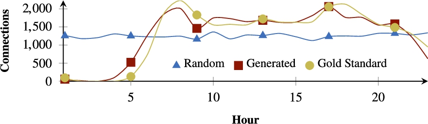
Connections per hour for the Belgian railway case.

Fig. 11.

Execution times when increasing the number of stops, routes or connections.

7.3. Performance

Metrics While performance is not the main focus of this work, we provide an indicative performance evaluation in this section in order to discover the bottlenecks and limitations of our current implementation that could be further investigated and resolved in future work. We measure the impact of different parameters on the execution times of the generator. The three main parameters for increasing the output dataset size are the number of stops, routes and connections. Because the number of edges is implicitly derived from the number of stops in order to reach a connected network, this can not be configured directly. In this section, we start from a set of parameters that produces realistic output data that is similar to the Belgian railway case. We let the value for each of these parameters increase to see the evolution of the execution times and memory usage.

Results Figure 11 shows a linear increase in execution times when increasing the routes or connections. The execution times for stops do however increase much faster, which is caused by the higher complexity of networks that are formed for many stops. The used algorithms for producing this network graph proves to be the main bottleneck when generating large networks. Networks with a limited size can however be generated quickly, for any number of routes and connections. The memory usage results from Fig. 12 also show a linear increase, but now the increase for routes and connections is higher than for the stops parameter. 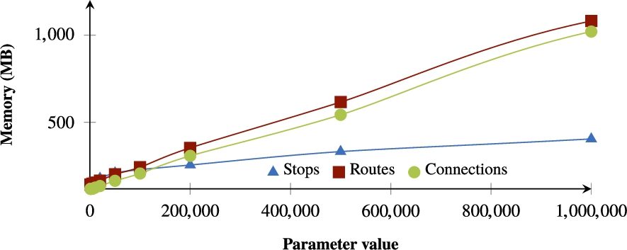These figures show that stops generation is a more cpu intensive process than routes and connections generation. These last two are able to make better usage of the available memory for speeding up the process.

Fig. 12.

Memory usage when increasing the number of stops, routes or connections.

7.4. Dataset size

An important aspect of dataset generation is its ability to output various dataset sizes. In podigg, different options are available for tweaking these sizes. Increasing the time range parameter within the generator increases the number of connections while the number of stops and routes will remain the same. When enlarging the geographical area over the same period of time, the opposite is true. As a rule of thumb, based on the number of triples per connection, stops and routes, the total number of generated triples per dataset is approximately $7 \cdot #connections + 6 \cdot #stops + #routes$ . For the Belgian railway case, containing 30,011 connections over a period of 9 months, with 583 stops and 362 routes, this would theoretically result in 213,937 triples. In practice, we reach 235,700 triples when running with these parameters, which is slightly higher because of the other triples that are not taken into account for this simplified formula, such as the ones for trips, stations and delays.

8. Discussion

In this section, we discuss the main characteristics, the usage within benchmarks and the limitations of this work. Finally, we mention several podigg use cases.

8.1. Characteristics

Our main research question on how to generate realistic synthetic public transport networks has been answered by the introduction of the mimicking algorithm from Section 5, based on commonly used practises in transit network design. This is based on the accepted hypothesis that the population distribution of an area is correlated with its transport network design and scheduling. We measured the realism of the generated datasets using the coherence metric in Section 7.1 and more fine-grained realism metrics for different public transport aspects in Section 7.2.

podigg, our implementation of the algorithm, accepts a wide range of parameters to configure the mimicking algorithm. podigg and podigg-lc are able to output the mimicked data respectively as gtfs and rdf datasets, together with a visualization of the generated transit network. Our system can be used without requiring any extensive setup or advanced programming skills, as it consists of simple command lines tools that can be invoked with a number of optional parameters to configure the generator. Our system is proven to be generalizable to other transport types, as we evaluated podigg for the bus and train transport type, and the Belgium and Netherlands geospatial regions in Section 7.2.

8.2. Usage within benchmarks

A synthetic dataset generator, which is one of the main contributions of this work, forms an essential aspect of benchmarks for (rdf) data management systems [2,19]. Prescribing a concrete benchmark that includes the evaluation of tasks is out of scope. However, to provide a guideline on how our dataset generator can be used as part of a benchmark, we relate the primary elements of public transport datasets to choke points in data management systems, i.e., key technical challenges in these system. Below, we list choke points related to storage and querying within data management systems and route planning systems. For each choke point, we introduce example tasks to evaluate them in the context of public transport datasets. The querying choke points are inspired by the choke points identified by Petzka et. al. [27] for faceted browsing.

Storage of entities.

Storage of stops, stations, connections, routes, trips and delays.

Storage of links between entities.

Storage of stops per station.

Storage of connections for stops.

Storage of the next connection for each connection.

Storage of connections per trip.

Storage of trips per route.

Storage of a connection per delay.

Storage of literals.

Storage of latitude, longitude, platform code and code of stops.

Storage of latitude, longitude and label of stations.

Storage of delay durations.

Storage of the start and end time of connections.

Storage of sequences.

Storage of sequences of connections.

Find instances by property value.

Find latitude, longitude, platform code or code by stop.

Find station by stop.

Find country by station.

Find latitude, longitude, or label by station.

Find delay by connection.

Find next connection by connection.

Find trip by connection.

Find route by connection.

Find route by trip.

Find instances by inverse property value.

Inverse of examples above.

Find instances by a combination of properties values.

Find stops by geospatial location.

Find stations by geospatial location.

Find instances for a certain property path with a certain value.

Find the delay value of the connection after a given connection.

Find the delay values of all connections after a given connection.

Find instances by inverse property path with a certain value.

Find stops that are part of a certain trip that passes by the stop at the given geospatial location.

Find instances by class, including subclasses.

Find delays of a certain class.

Find instances with a numerical value within a certain interval.

Find stops by latitude or longitude range.

Find stations by latitude or longitude range.

Find delays with durations within a certain range.

Find instances with a combination of numerical values within a certain interval.

Find stops by geospatial range.

Find stations by geospatial range.

Find instances with a numerical interval by a certain value for a certain property path.

Find connections that pass by stops in a given geospatial range.

Find instances with a numerical interval by a certain value.

Find connections that occur at a certain time.

Find instances with a numerical interval by a certain value for a certain property path.

Find trips that occur at a certain time.

Find instances with a numerical interval by a certain interval.

Find connections that occur during a certain time interval.

Find instances with a numerical interval by a certain interval for a certain property path.

Find trips that occur during a certain time interval.

Find instances with numerical intervals by intervals with property paths.

Find connections that occur during a certain time interval with stations that have stops in a given geospatial range.

Find trips that occur during a certain time interval with stops in a given geospatial range.

Plan a route that gets me from stop A to stop B starting at a certain time.

This list of choke points and tasks can be used as a basis for benchmarking spatiotemporal data management systems using public transport datasets. For example, sparql queries can be developed based on these tasks and executed by systems using a public transport dataset. For the benchmarking with these tasks, it is essential that the used datasets are realistic, as discussed in Section 7.2. Otherwise, certain choke points may not resemble the real world. For example, if an unrealistic dataset would contain only a single trip that goes over all stops, then finding a route between two given stops could be unrealistically simple.

8.3. Limitations and future work

In this section, we discuss the limitations of the current mimicking algorithm and its implementation, together with further research opportunities.

Memory usage The sequential steps in the presented mimicking algorithm require persistence of the intermediary data that is generated in each step. Currently, podigg is implemented in such a way that all data is kept in-memory for the duration of the generation, until it is serialized. When large datasets need to be generated, this requires a larger amount of memory to be allocated to the generator. Especially for large amounts of routes or connections, where 100 million connections already require almost 10 GB of memory to be allocated. While performance was not the primary concern in this work, in future work, improvements could be made in the future. A first possible solution would be to use a memory-mapped database for intermediary data, so that not all data must remain in memory at all times. An alternative solution would be to modify the mimicking process to a streaming algorithm, so that only small parts of data need to be kept in memory for datasets of any size. Considering the complexity of transit networks, a pure streaming algorithm might not be feasible, because route design requires knowledge of the whole network. The generation of connections however, could be adapted so that it works as a streaming algorithm.

Realism We aimed to produce realistic transit feeds by reusing the methodologies learned in public transit planning. Our current evaluation compares generated output to real datasets, as no similar generators currently exist. When similar generation algorithms are introduced in the future, this evaluation can be extended to compare their levels of realism. Our results showed that all sub-generators, except for the trips generator, produced output with a high realism value. The trips are still closer to real data than a random generator, but this can be further improved in future work. This can be done by for instance taking into account network capacities [20] on certain edges when instantiating routes as trips, because we currently assume infinite edge capacities, which can result in a large amount of connections over an edge at the same time, which may not be realistic for certain networks. Alternatively, we could include other factors in the generation algorithm, such as the location of certain points of interest, such as shopping areas, schools and tourist spots. In the future, a study could be done to identify and measure the impact of certain points of interest on transit networks, which could be used as additional input to the generation algorithm to further improve the level of realism. Next to this, in order to improve transfer coordination [20], possible transfers between trips should be taken into account when generating stop times. Limiting the network capacity will also lead to natural congestion of networks [8], which should also be taken into account for improving the realism. Furthermore, the total vehicle fleet size [20] should be considered, because we currently assume an infinite number of available vehicles. It is more realistic to have a limited availability of vehicles in a network, with the last position of each vehicle being of importance when choosing the next trip for that vehicle.

Alternative implementations An alternative way of implementing this generator would be to define declarative dependency rules for public transport networks, based on the work by Pengyue et. al. [25]. This would require a semantic extension to the engine so that is aware of the relevant ontologies and that it can serialize to one or more rdf formats. Alternatively, machine learning techniques could be used to automatically learn the structure and characteristics of real datasets and create similar realistic synthetic datasets [16], or to create variants of existing datasets [31]. The downside of machine learning techniques is however that it is typically more difficult to tweak parameters of automatically learned models when specific characteristics of the output need to be changed, when compared to a manually implemented algorithm. Sensitivity analysis could help to determine the impact of such parameters in order to understand the learned models better.

Streaming extension Finally, the temporal aspect of public transport networks is useful for the domain of rdf stream processing [12]. Instead of producing single static datasets as output, podigg could be adapted to produce rdf streams of connections and delays, where information about stops and routes are part of the background knowledge. Such an extension can become part of a benchmark, such as CityBench [1] and LSBench [24], for assessing the performance of rdf stream processing systems with temporal and geospatial capabilities.

8.4. podigg in use

podigg and podigg-lc have been developed for usage within the hobbit platform. This platform is being developed within the hobbit project and aims to provide an environment for benchmarking rdf systems for Big Linked Data. The platform provides several default dataset generators, including podigg, which can be used to benchmark systems.

podigg, and its generated datasets are being used in the eswc Mighty Storage Challenge 2017 and 2018 [18]. The first task of this challenge consists of rdf data ingestion into triple stores, and querying over this data. Because of the temporal aspect of public transport data in the form of connections, podigg datasets are fragmented by connection departure time, and transformed to a data stream that can be inserted. In task 4 of this challenge, the efficiency of faceted browsing solutions is benchmarked [27]. In this work, a list of choke points are identified regarding sparql queries on triple stores, which includes points such as the selection of subclasses and property-path transitions. Because of the geographical property of public transport data, podigg datasets are being used for this benchmark.

Finally, podigg is being used for creating virtual transit networks of variable size for the purposes of benchmarking route planning frameworks, such as Linked Connections [10].

9. Conclusions

In this article, we introduced a mimicking algorithm for public transport data, based on steps that are used in real-world transit planning. Our method splits this process into several sub-generators and uses population distributions of an area as input. As part of this article, we introduced podigg, a reusable framework that accepts a wide range of parameters to configure the generation algorithm.

Results show that the structuredness of generated datasets are similar to real public transport datasets. Furthermore, we introduced several functions for measuring the realism of synthetic public transport datasets compared to a gold standard on several levels, based on distance functions. The realism was confirmed for different regions and transport types. Finally, the execution times and memory usages were measured when increasing the most important parameters, which showed a linear increase for each parameter, showing that the generator is able to scale to large dataset outputs.

The public transport mimicking algorithm we introduced, with podigg and podigg-lc as implementations, is essential for properly benchmarking the efficiency and performance of public transport route planning systems under a wide range of realistic, but synthetic circumstances. Flexible configuration allows datasets of any size to be created and various characteristics to be tweaked to achieve highly specialized datasets for testing specific use cases. In general, our dataset generator can be used for the benchmarking of geospatial and temporal rdf data management systems, and therefore lowers the barrier towards more efficient and performant systems.

Footnotes

Acknowledgement

We wish to thank Henning Petzka for his help with discovering issues and providing useful suggestions for the podigg implementation. The described research activities were funded by the H2020 project hobbit (#688227).

References

M.I.

Ali ,

Gao and

Mileo , CityBench: A configurable benchmark to evaluate rsp engines using smart city datasets, in: International Semantic Web Conference,

Arenas ,

Corcho ,

Simperl ,

Strohmaier ,

d’Aquin ,

Srinivas ,

Groth ,

Dumontier ,

Heflin ,

Thirunarayan and

Staab , eds, Springer International Publishing, Cham, 2015, pp. 374–389.

Angles ,

Boncz ,

Larriba-Pey ,

Fundulaki ,

Neumann ,

Erling ,

Neubauer ,

Martinez-Bazan ,

Kotsev and

Toma , The linked data benchmark council: A graph and rdf industry benchmarking effort, ACM SIGMOD Record43(1) (2014), 27–31. doi:10.1145/2627692.2627697.

D.F.

Barbieri ,

Braga ,

Ceri ,

Della Valle and

Grossniklaus , C-sparql: sparql for continuous querying, in: Proceedings of the 18th International Conference on World Wide Web, ACM, 2009, pp. 1061–1062. doi:10.1145/1526709.1526856.

Bast ,

Hertel and

Storandt , Scalable transfer patterns, in: 2016 Proceedings of the Eighteenth Workshop on Algorithm Engineering and Experiments (ALENEX), 2016, pp. 15–29. doi:10.1137/1.9781611974317.2.

Battle and

Kolas , Enabling the geospatial semantic web with Parliament and geosparql, Semantic Web3(4) (2012), 355–370. doi:10.3233/SW-2012-0065.

Berners-Lee , Linked Data, 2006.

Bizer and

Schultz , The Berlin sparql benchmark, International Journal on Semantic Web and Information Systems5(2) (2009), 1–24. doi:10.4018/jswis.2009040101.

Brinkhoff , A framework for generating network-based moving objects, GeoInformatica6(2) (2002), 153–180. doi:10.1023/A:1015231126594.

Colpaert ,

Chua ,

Verborgh ,

Mannens ,

Van de Walle and

Vande Moere , What public transit api logs tell us about travel flows, in: Proceedings of the 6 ^th USEWOD Workshop on Usage Analysis and the Web of Data, WWW ’16 Companion , International World Wide Web Conferences Steering Committee, Republic and Canton of Geneva, Switzerland, 2016, pp. 873–878. doi:10.1145/2872518.2891069.

10.

Colpaert ,

Llaves ,

Verborgh ,

Corcho ,

Mannens and

Van de Walle , Intermodal public transit routing using linked connections, in: Proceedings of the 14th International Semantic Web Conference: Posters and Demos, 2015, pp. 1–5.

11.

Cyganiak ,

Wood and

Lanthaler , rdf 1.1: Concepts and abstract syntax, Recommendation W3C (2014).

12.

Della Valle ,

Ceri ,

van Harmelen and

Fensel , It’s a streaming world! Reasoning upon rapidly changing information, Intelligent Systems, IEEE24(6) (2009), 83–89. doi:10.1109/MIS.2009.125.

13.

Delling ,

Sanders ,

Schultes and

Wagner , Engineering route planning algorithms, in: Algorithmics of Large and Complex Networks: Design, Analysis, and Simulation,

Lerner,

Wagner and

K.A.

Zweig , eds, Springer Berlin Heidelberg, Berlin, Heidelberg, 2009, pp. 117–139. doi:10.1007/978-3-642-02094-0_7.

14.

Dibbelt ,

Pajor ,

Strasser and

Wagner , Intriguingly simple and fast transit routing, in: Experimental Algorithms,

Bonifaci ,

Demetrescu and

Marchetti-Spaccamela , eds, Springer Berlin Heidelberg, Berlin, Heidelberg, 2013, pp. 43–54. doi:10.1007/978-3-642-38527-8_6.

15.

Duan ,

Kementsietsidis ,

Srinivas and

Udrea , Apples and oranges: A comparison of rdf benchmarks and real rdf datasets, in: Proceedings of the 2011 ACM SIGMOD International Conference on Management of Data, SIGMOD ’11, New York, NY, USA, 2011, pp. 145–156, ACM. doi:10.1145/1989323.1989340.

16.

Eno and

C.W.

Thompson , Generating synthetic data to match data mining patterns, IEEE Internet Computing12(3) (2008), 78–82. doi:10.1109/MIC.2008.55.

17.

Garbis ,

Kyzirakos and

Koubarakis , Geographica: A benchmark for geospatial rdf stores, in: Proceedings of the 12th International Semantic Web Conference,

Alani ,

Kagal ,

Fokoue ,

Groth ,

Biemann ,

J.X.

Parreira ,

Aroyo ,

Noy ,

Welty and

Janowicz , eds, Springer Berlin Heidelberg, Berlin, Heidelberg, 2013, pp. 343–359. doi:10.1007/978-3-642-41338-4_22.

18.

Georgala ,

Spasić ,

Jovanovik ,

Petzka ,

Röder and

A.-C.N.

Ngomo , MOCHA2017: The mighty storage challenge at eswc 2017, in: Semantic Web Challenges,

Dragoni ,

Solanki and

Blomqvist , eds, Springer International Publishing, Cham, 2017, pp. 3–15. doi:10.1007/978-3-319-69146-6_1.

19.

Gray , Benchmark Handbook: For Database and Transaction Processing Systems, Morgan Kaufmann Publishers Inc., San Francisco, CA, USA, 1992.

20.

Guihaire and

J.-K.

Hao , Transit network design and scheduling: A global review, Transportation Research Part A: Policy and Practice42(10) (2008), 1251–1273. doi:10.1016/j.tra.2008.03.011.

21.

Guo ,

Pan and

Heflin , LUBM: A benchmark for owl knowledge base systems, in: Web Semantics: Science, Services and Agents on the World Wide Web, Vol. 3, 2005, pp. 158–182. doi:10.1016/j.websem.2005.06.005.

22.

Kyzirakos ,

Karpathiotakis and

Koubarakis , Strabon: A semantic geospatial dbms, in: The Semantic Web – ISWC 2012,

Cudré-Mauroux ,

Heflin ,

Sirin ,

Tudorache ,

Euzenat ,

Hauswirth ,

J.X.

Parreira ,

Hendler ,

Schreiber ,

Bernstein and

Blomqvist , eds, Springer Berlin Heidelberg, Berlin, Heidelberg, 2012, pp. 295–311. doi:10.1007/978-3-642-35176-1_19.

23.

Le-Phuoc ,

Dao-Tran ,

J.X.

Parreira and

Hauswirth , A native and adaptive approach for unified processing of Linked Streams and Linked Data, in: The Semantic Web – ISWC 2011,

Aroyo ,

Welty ,

Alani ,

Taylor ,

Bernstein ,

Kagal ,

Noy and

Blomqvist , eds, Springer Berlin Heidelberg, Berlin, Heidelberg, 2011, pp. 370–388. doi:10.1007/978-3-642-25073-6_24.

24.

Le-Phuoc ,

Dao-Tran ,

M.-D.

Pham ,

Boncz ,

Eiter and

Fink , Linked stream data processing engines: Facts and figures, in: The Semantic Web – ISWC 2012,

Cudré-Mauroux ,

Heflin ,

Sirin ,

Tudorache ,

Euzenat ,

Hauswirth ,

J.X.

Parreira ,

Hendler ,

Schreiber ,

Bernstein and

Blomqvist , eds, Springer Berlin Heidelberg, Berlin, Heidelberg, 2012, pp. 300–312. doi:10.1007/978-3-642-35173-0_20.

25.

P.J.

Lin ,

Samadi ,

Cipolone ,

D.R.

Jeske ,

Cox ,

Rendon ,

Holt and

Xiao , Development of a synthetic data set generator for building and testing information discovery systems, in: Third International Conference on Information Technology: New Generations (ITNG’06), IEEE, 2006, pp. 707–712. doi:10.1109/ITNG.2006.51.

26.

M.A.

Nascimento ,

Pfoser and

Theodoridis , Synthetic and real spatiotemporal datasets, IEEE Data Eng. Bull.26(2) (2003), 26–32.

27.

Petzka ,

Stadler ,

Katsimpras ,

Haarmann and

Lehmann , Benchmarking faceted browsing capabilities of triplestores, in: Proceedings of the 13th International Conference on Semantic Systems, 2017, pp. 128–135. doi:10.1145/3132218.3132242.

28.

Pyrga ,

Schulz ,

Wagner and

Zaroliagis , Efficient models for timetable information in public transportation systems, Journal of Experimental Algorithmics (JEA)12 (2008), 2–4. doi:10.1145/1227161.1227166.

29.

Schmidt ,

Hornung ,

Lausen and

Pinkel , SP²bench: A sparql performance benchmark, in: 2009 IEEE 25th International Conference on Data Engineering, IEEE, 2009, pp. 222–233. doi:10.1109/ICDE.2009.28.

30.

Spasić ,

Jovanovik and

Prat-Pérez , An rdf dataset generator for the social network benchmark with real-world coherence, in: Proceedings of the Workshop on Benchmarking Linked Data, Volume 1700 of Ceur Workshop Proceedings,

Fundulaki ,

Krithara ,

A.-C.

Ngonga Ngomo and

Rentoumi , eds, 2016.

31.

S.C.

Wong ,

Gatt ,

Stamatescu and

M.D.

McDonnell , Understanding data augmentation for classification: When to warp? in: Digital Image Computing: Techniques and Applications (DICTA), 2016 International Conference on, IEEE, 2016, pp. 1–6.

Generating public transport data based on population distributions for RDF benchmarking

Abstract

Keywords

1. Introduction

2. Related work

1 http://project-hobbit.eu/

3.1. Public transit planning

3.2. Transit feed formats

2 https://developers.google.com/transit/gtfs/

3 p-values in both cases < 0.00001 .

5.1. Region

5.5. Trips

6 https://hello.irail.be

8 http://vocab.gtfs.org/terms

14 https://github.com/PoDiGG/podigg-lc

19 https://github.com/PoDiGG/podigg#parameters

20 https://github.com/PoDiGG/podigg-evaluate

21 https://github.com/PoDiGG/graph-coherence

22 https://github.com/PoDiGG/population-density-generator

8. Discussion

8.1. Characteristics

8.2. Usage within benchmarks

8.3. Limitations and future work

8.4. podigg in use

9. Conclusions

Footnotes

Acknowledgement

References

¹
http://project-hobbit.eu/

²
https://developers.google.com/transit/gtfs/

³
p-values in both cases $< 0.00001$ .

⁶
https://hello.irail.be

⁸
http://vocab.gtfs.org/terms

¹⁴
https://github.com/PoDiGG/podigg-lc

¹⁹
https://github.com/PoDiGG/podigg#parameters

²⁰
https://github.com/PoDiGG/podigg-evaluate

²¹
https://github.com/PoDiGG/graph-coherence

²²
https://github.com/PoDiGG/population-density-generator