Topic profiling benchmarks in the linked open data cloud: Issues and lessons learned

Abstract

Topical profiling of the datasets contained in the Linking Open Data (LOD) cloud has been of interest since such kind of data became available within the Web. Different automatic classification approaches have been proposed in the past, in order to overcome the manual task of assigning topics for each and every individual (new) dataset. Although the quality of those automated approaches is comparably sufficient, it has been shown, that in most cases a single topical label per dataset does not capture the topics described by the content of the dataset. Therefore, within the following study, we introduce a machine-learning based approach in order to assign a single topic, as well as multiple topics for one LOD dataset and evaluate the results. As part of this work, we present the first multi-topic classification benchmark for LOD cloud datasets, which is freely accessible. In addition, the article discusses the challenges and obstacles, which need to be addressed when building such a benchmark.

1. Introduction

In 2006, Tim-Berners Lee [5] introduced the Linked Open Data paradigm. It refers to a set of best practices for publishing and connecting structured data on the Web. The adoption of such best practices assures that the structure and the semantics of the data are made explicit which is also the main goal of the Semantic Web. Datasets, which should be published as Linked Data, need to comply to a set of rules to ensure an easy discoverability, as well as an easy way to query information within the dataset [6]. Therefore, LOD datasets should be published adopting W3C1

¹

https://www.w3.org/

standards in the RDF2 ²

https://www.w3.org/RDF/

format and providing a SPARQL3 ³

http://www.w3.org/TR/rdf-sparql-query/

endpoint to query them. Over the last few years, the overall spread of datasets being part of the LOD cloud has increased from 12 datasets in 2007, to more than 1000 datasets as of April 2014 [35], where the overall number is constantly increasing. These datasets4 ⁴

http://linkeddatacatalog.dws.informatik.uni-mannheim.de/state/

cover different domains which is shown by the different colors in the LOD cloud described in Fig. 1. Although publishing such amounts of data adopting the principles of Linked Data has many advantages, its consumption is still limited.

The process of exploring Linked Data for a given topic is long and not intuitive. In an ideal scenario, a user decision whether to use a dataset or not, is based on the information (e.g., topic) provided in the metadata. In this setup, no initial querying of the information contained in the dataset is required. But especially in those cases when datasets do not provide metadata information about their topic/s, a lot of exploration steps are required in order to understand if the information contained in the dataset is useful or not.

The datasets in the LOD cloud 2014 belong to different domains, with social media, government data, and publications data being the most prominent areas [35]. For every dataset in the cloud, the topic is either assigned by verifying its content or by accessing the metadata assigned by the publisher. Up until now, topical categories have been manually assigned to LOD datasets either by the publishers of the datasets themselves via the datahub.io dataset catalog or by the authors of the LOD cloud [35]. For some datasets published as LOD such as Linked Movie Database,5 ⁵

http://www.linkedmdb.org/

or GeoNames6 ⁶

http://www.geonames.org/

the metadata is completely missing, while for some others e.g., DBpedia7 ⁷

http://www.dbpedia.org

the topics it covers are not explicitly described.

The topic of a dataset can be defined as the subject of the dataset, i.e. the subject or theme of a discourse of one of its parts.

It is very important to have a classification of datasets according to their topical domain not only to judge whether it is useful for the use case at hand or not but also as shown in [35], it is often interesting to analyze characteristics of datasets clustered by topical domains, so that trends and best practices that exist only in a particular topical domain can be identified. Link discovery also can be supported by knowing the topic of the dataset. Datasets that share the same topic, probably share equivalent instances. Topical classification is also important for coloring of the Linked Data cloud as in Fig. 1, which marks datasets according to their topical domain.

Even though the importance of topic profiling of Linked Data is undoubtful, it has not yet received sufficient attention from the Linked Data community and it poses a number of unique challenges:

• Linked Data comes from different autonomous sources and is continuously evolving. The descriptive information or the metadata depend on the data publishers’ will. Often publishers are more interested in publishing their data in RDF format and do not focus sufficiently on the right meta information. Moreover, data publishers face difficulties in using appropriate terms for the data to be described. Apart from a well-known group of vocabularies, it is difficult to find vocabularies for most of the domains that would be a good candidate for the dataset at hand, as evaluated in [42].

• Billions of triples is a daunting scale that poses very high performance and scalability demands. Managing the large and rapidly increasing volume of data is being a challenge for developing techniques that scale well with the volume of data in the LOD cloud.

• The high volume of data demands that data consumers develop automatic approaches to assign the topic of the datasets.

• Topic profiling techniques should deal with structural, semantic and schema heterogeneity of the LOD datasets.

• Querying or browsing data in the LOD cloud is challenging, because the metadata is often not structured and not in a machine-readable format. A data consumer who wants to select for example, all datasets that belong to the media category faces such challenge.

Topic profiling approaches can be evaluated with topic benchmarking datasets. In general, benchmarks provide an experimental basis for evaluating software engineering theories, represented by software engineering techniques, in an objective and repeatable manner [14]. A benchmark therefor is defined as a procedure, problem, or test that can be used to compare systems or components to each other or to a standard [31]. A benchmark represents research problems of interest and solutions of importance in a research area through the definition of the motivating comparison, task sample and evaluation measures [36]. The capability to compare the efficiency and/or effectiveness of different solutions for the same task is a key enabling factor in both industry and research. Moreover, in many research areas the possibility to replicate existing results provided in the literature is one of the pillars of the scientific method. In the ICT field, benchmarks are the tools which support both comparison and reproducibility tasks. In the database community, the benchmark series defined by the TPC8 ⁸

http://www.tpc.org

is a very famous example. Topic benchmarks over Linked Data are important for several reasons; (i) they allow developers to assess the performance of their tool; (ii) help to compare the different available tools that exist and evaluate the suitability for their needs; and (iii) researchers can address new challenges. Despite the importance of such needs, topic benchmarking over Linked Data is relatively new. This is also reflected in the fact that there is no gold standard for topic classification of LOD datasets as described in Section 10.

This paper presents our experience in designing and using a new benchmark for multi-topic profiling and discuss the choke points which influence the performance of such systems. In [25], we investigated to which extent we can automatically classify datasets from the LOD cloud into a single topic category. We make use of the LOD cloud data collection of 2014 [35] to train different classifiers for determining the topic of a dataset. In this paper, we also report the results achieved from the experiments for single-topic classification of LOD datasets [25], with the aim to provide the reader a complete view of the datasets, experiments and analysis of the results. Learning from the results of the previous experiments as most of the datasets expose more than one topic, we further investigate the problem of multi-topic classification of LOD datasets by extending the original benchmark by adding to some of the datasets more than one topic. Results of this new benchmark are not satisfactory due to the nature of the content of selected datasets and the topics’ choice (taken for the original benchmark). We provide a comprehensive analysis of the challenges and line out our learned lessons on this very complex and relevant task. The benchmark, together with various feature extracted from the different datasets, as well as the results of our experiments (described in this paper) are publicly available. We hope to help the LOD community to improve existing techniques for topic benchmark creation and evaluation and encourage new research in this area.

The remaining of the article is organized as follows: In Section 2, we give the definition for topic; single and multi-topic classification. Section 3 describes the criteria for developing a sufficient and comprehensive benchmark and how our benchmark meets such criteria. In Section 4, the methodology for creating the benchmark is discussed, where the following section reports the data corpus that was used in our experiments. Section 6 describes the extraction of different features that characterize the LOD datasets and introduces the different classification algorithms used for the classification. Section 7 discusses the performance metrics used to evaluate our benchmark. In Section 8, we present the result of the experiments in order to evaluate the benchmark for multi-topic classification. Section 9 reports the analysis of the results in depth and the lessons learned, while in Section 10 the state-of-the-art in topic profiling and topic benchmarking are discussed. Finally, in Section 11, we draw conclusions and present future directions.

Fig. 1.

Linked Data (LOD) Cloud.

2. Topic definition

Given a large RDF dataset with heterogeneous content, we want to derive the topic or topics that can be understood as the subject/s of the dataset by using different feature vectors that describe the characteristics of the data.

Definition 1 (Topical category).

Given a set of RDF triples $\mathrm{(}\mathit{s}\mathrm{,}\mathit{p}\mathrm{,}\mathit{o}\mathrm{)}$ , a topic T is a label ${\mathit{l}}_{\mathit{j}}$ from a set of labels $\mathit{L}=\{{\mathit{l}}_1\mathrm{,}{\mathit{l}}_2\mathrm{,}\dots \mathrm{,}{\mathit{l}}_{\mathit{p}}\}$ that describes the content of the dataset relating it with a specific area of the real world. Often a dataset can have more than one topic meaning that a subset of labels ${\mathit{l}}_{\mathit{k}}\subseteq \mathit{L}$ , where $\mathit{k}=1\mathrm{,}\dots \mathrm{,}\mathit{p}$ is the set of p possible topics.

Definition 2 (Single-topic classification).

Given a set $\{{\mathit{D}}_1\mathrm{,}{\mathit{D}}_2\mathrm{,}\dots \mathrm{,}{\mathit{D}}_{\mathit{N}}\}$ of datasets, where each ${\mathit{D}}_{\mathit{i}}$ is associated with a feature vector ${\mathit{x}}_{\mathit{i}}=\mathrm{(}{\mathit{x}}_{\mathit{i}1}\mathrm{,}{\mathit{x}}_{\mathit{i}2}\mathrm{,}\dots \mathrm{,}{\mathit{x}}_{\mathit{i}\mathit{M}}\mathrm{)}$ , the process of assigning only a single label ${\mathit{l}}_{\mathit{j}}$ from the set of labels $\{{\mathit{l}}_1\mathrm{,}{\mathit{l}}_2\mathrm{,}\dots \mathrm{,}{\mathit{l}}_{\mathit{p}}\}$ to ${\mathit{D}}_{\mathit{i}}$ , is called single-topic classification.

Definition 3 (Multi-topic classification).

Given a set $\{{\mathit{D}}_1\mathrm{,}{\mathit{D}}_2\mathrm{,}\dots \mathrm{,}{\mathit{D}}_{\mathit{N}}\}$ of datasets, where each ${\mathit{D}}_{\mathit{i}}$ is associated with a feature vector ${\mathit{x}}_{\mathit{i}}=\mathrm{(}{\mathit{x}}_{\mathit{i}1}\mathrm{,}{\mathit{x}}_{\mathit{i}2}\mathrm{,}\dots \mathrm{,}{\mathit{x}}_{\mathit{i}\mathit{M}}\mathrm{)}$ , the process of assigning a subset of labels ${\mathit{l}}_{\mathit{k}}\subseteq \mathit{L}$ to ${\mathit{D}}_{\mathit{i}}$ , is called multi-topic classification.

For creating the diagram in Fig. 1, the newly discovered datasets were manually annotated with one of the following topical categories: media, government, publications, life sciences, geographic, cross-domain, user generated content, and social networking [35].

The media category contains datasets providing information about films, music, TV and radio programmes, as well as printed media. Some datasets in this category are the dbtune.org music dataset, the New York Times dataset, and the BBC radio and television program datasets.

The government category contains Linked Data published by federal or local governments, including a lot of statistical datasets. Examples of the datasets in this category include the data.gov.uk and opendatacommunities.org dataset.

The publications category holds information library datasets, information about scientific publications and conferences, reading lists from universities, and citation database. Prominent datasets in this category include German National Library dataset, the L3S DBLP dataset and the Open Library dataset.

The geographic category contains datasets like geonames.org and linkedgeodata.org comprising information about geographic entities, geopolitical divisions and points of interest.

The life science category comprises biological and biochemical information, drug-related data, and information about species and their habitats. Examples of datasets that belong to this category are Drugbank FU-Berlin, Geospecies and Biomodels RDF.

The cross-domain category includes general knowledge bases such as DBpedia or UMBEL, linguistic resources such as WordNet or Lexvo, as well as product data.

The user-generated content category contains data from portals that collect content generated by larger user communities. Examples include metadata about blogposts published as Linked Data by wordpress.com, data about open source software projects published by apache.org, scientific workflows published by myexperiment.org, and reviews published by goodreads.com or revyu.com.

The social networking category contains people profile as well as data describing the social ties among people. In this category individual FOAF profiles are included, as well as data about the interconnections among users of the distributed microblogging platform StatusNet.

3. Desiderata for benchmark

Benchmarking is the continuous, systematic process of measuring one’s output and/or work processes against the toughest competitors or those recognized best in the industry [9]. The benefits of having a benchmark are many among which:

1. It helps organizations understand strengths and weaknesses of solutions.

2. By establishing new standards and goals a benchmark helps in better satisfying the customers’ needs.

3. Motivates to reach new standards and to keep on new developments.

4. Allows organizations to realize what level(s) of performance is really possible by looking at others.

5. Is a cost-effective and time-efficient way of establishing innovative ideas.

[36] describes seven properties that a good benchmark should consider; accessibility, relevance, affordability, portability, scalability, clarity and solvability. In the following, we describe each of the aspects in building our benchmark. Accessibility:

One of the most important characteristics of the benchmark is to make it easy to obtain and use. The data and the results need to be publicly available so that anyone can apply their tools and techniques on the benchmark and compare their results with others. This characteristic is very important because it allows users to easily interpret benchmark results.

Relevance:

A good benchmark should clearly define the intended use and the applicable scenarios. Our benchmark is understandable to a large audience and covers the topics that already exist in the Linked Open Data cloud.

Affordability:

The developed benchmark’s cost should be affordable and comparable to the value of the results. To complete the benchmark for a single combination of the workload takes 15 to 240 minutes.

Portability:

The tasks consist of stand-alone Java projects containing required libraries, making thus the platform portability not a challenge for our benchmark.

Scalability:

The benchmark should be scalable to work with tools and techniques at different levels of maturity.

Clarity:

The documentation for the benchmark should be clear and concise. The documentation for the topic benchmarking of LOD dataset is provided at https://github.com/Blespa/TopicalProfiling for evaluation and comparison to ensure repeatability and disclosure. Along with the benchmark we provide also an analysis as part of the benchmark materials in order to solve those issues which do not follow classification rules.

Solvability:

The benchmark should produce a good solution. The proposed benchmark resolves the task of multi-topic classification of LOD datasets, a task that is achievable but not trivial. Thus, our benchmark provides an opportunity for systems to show their capabilities and their shortcomings.

4. Benchmark development methodology

The development of the topic benchmark results in the creation of three elements:

• Data corpus the set of RDF datasets used by the benchmark.

• Workload which defines the set of operations that the system under benchmarking has to perform during the benchmark execution.

• Performance metrics which are used to measure quantitatively the performance of the systems.

On one hand, a benchmark models a particular scenario, meaning that the users of the benchmark must be able to understand the scenario and believe that this use case matches a larger class of use cases appearing in practice. On the other hand, a benchmark exposes technology to overload. A benchmark is valuable if its workload stresses important technical functionality of the actual systems called choke points. In order to understand and analyze choke points an intimate knowledge of the actual system architecture and workload is needed. In this paper, we identify and analyze choke points of the topic benchmarks and discuss the possibilities to optimize such benchmarks. Choke points can ensure that existing techniques are present in a system, but can also be used to reward future systems that improve performance on still open technical challenges [2].

For the single topic classification we used as benchmark the information that is currently used in the LOD cloud, as the topic for each dataset was manually assigned, while for the multi-topic classification due to the lack of presence of a benchmark we create one. Based on the results of the single-topic classification of LOD datasets, for the development of the multi-topic benchmark we consider some criteria for the selection of the datasets such as; size, number of different data-level descriptors (called feature vectors, see Section  6.1 ), and non-overlap of topics.

We select 200 datasets randomly from the whole set of datasets contained in the LOD cloud of 2014. In the selection of the datasets, we consider small-size datasets (less than 500 triples), medium-size datasets (between 501 and 5000 triples) and big-size datasets (more than 5000 triples). As we investigate schema level information we also take into consideration the number of different attributes for each feature vector used as input in our approach. For example, if a dataset uses less than 20 different vocabularies it is considered in the group of weak-schema descriptors; using between 20 and 200 different vocabularies are considered lite-schema descriptors and datasets that make use of more than 200 vocabularies are categorized as strong-schema descriptors.

Another criteria for building our benchmark is the non-overlap of topics. The distinction between two topical categories in the LOD cloud social networking and user-generated content is not straightforward as it is not clear what datasets should go into each of them. User-generated content can cover different topical domains thus to avoid misclassification of datasets we remove this category from the list of topical categories for LOD datasets. We face the same problem when classifying datasets into the cross-domain category and any other category. Because under the cross-domain category, also datasets in life science domain, or media domain can be categorized, we removed this category from the list of topics that we used for the multi-topic classification of LOD datasets. From eight categories in the single topic experiments, in the multi-topic classification we have only six categories life science, government, media, publications, social networking and geographic.

Two researchers were involved for this task. They independently classified datasets in the LOD into more than one category. To assign more than one topical category to each dataset the researchers could access the descriptive metadata published into Mannheim Linked Data Catalog9

⁹

http://linkeddatacatalog.dws.informatik.uni-mannheim.de/

which represents the metadata in the form of tags. Also, they had the possibility to take a deeper look inside the data itself. From the results, the researchers had an inter-rater agreement of $95.64\mathrm{\%}$ . Cases for which the assigned topics differ between the two researchers were further discussed with two professors.

Table 1

Distribution of number datasets per number of topics

Number of topics	1	2	3	4	5
Number of datasets	85	87	22	4	2

Table 1 shows the distribution of the number of datasets by the number of topics. As we can see, in our benchmark for the multi-topic classification, most of the datasets have one or two topics, while less than $3\mathrm{\%}$ of the datasets have more than four topics.

The benchmark that we build for the multi-topic classification of LOD datasets is available for further research in this topic.10 ¹⁰

https://github.com/Blespa/TopicalProfiling

5. Data corpus

In order to build up the benchmark, which is described within this article, we made use of the crawl of Linked Data referred to April 2014 by [35]. The authors used the LD-Spider crawler originally designed by [16], which follows dataset interlinks to crawl LOD. The crawler seeds originate from three resources:

1. Datasets from the lod-cloud in datahub.io datasets catalog, as well as other datasets marked with Linked Data related tags within the same catalog

2. A sample from the Billion Triple Challenge 2012 dataset11

   ¹¹

   http://km.aifb.kit.edu/projects/btc-2012/

   Datasets advertised since 2011 in the mailing list of public-lodw3.org

   The crawled data contained 900129 documents describing 8038396 resources with altogether around 188 million RDF triples. To group all the resources in datasets, it was assumed that all the data originating by one pay-level domain (PLD) belong to a single dataset. The gathered data originates from 1024 different datasets from the Web and is publicly available.12 ¹²

   http://data.dws.informatik.uni-mannheim.de/lodcloud/2014/ISWC-RDB/

   Figure 2 shows the distribution of the number of resources and documents per dataset contained in the crawl.

   

   Fig. 2.

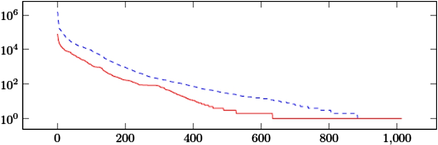
   Distribution of the number of resources and documents (log scale) per dataset contained in the crawl.

   The authors of the 2014 LOD cloud [35] make a distinction between the two categories user-generated content and social networking. Datasets in the first category focus on the actual content while datasets in the second category focus on user profiles and social ties.

   The distribution of categories within the datasets of the LOD cloud is shown in Fig. 3. As we can see, the cloud is dominated by datasets from the social networking category, followed by government datasets. Only less than 25 datasets are included in the cloud for each of the domains media and geographic. The topical category is manually assigned to each dataset in the LOD cloud thus we consider it as a gold standard for our experiments. The imbalance needs to be taken into account for the later model learning, as some classification algorithms tend to predict better for stronger represented classes.

   

   Fig. 3.

   Topics Distribution within LOD Cloud Datasets.

   6. Workload

   In the following, we describe in detail the process of feature extraction, which we apply for our task in assigning more than one topic to LOD datasets. First, we present the created feature vectors, which were extracted from the datasets. In the second part of this section we describe the classification algorithms, as well as the sampling and normalization techniques which were used.

   6.1. Feature vectors

   For each of the datasets contained in our collection, we derive attributes/features from ten different sources (e.g., the URI of the dataset, or the used vocabulary) which are described in the following:

   Vocabulary Usage (VOC):

   As vocabularies mostly describe a set of classes for a particular domain, e.g. foaf for describing persons, or bibo for bibliographic information, we assume that the vocabularies used by a dataset form a helpful indicator for determining the topical category of the dataset. We extract the predicates and classes which represent the set of terms of the vocabularies used by the dataset. We determine the vocabularies by aggregating the namespaces of these terms. We then sum up the number of occurrences resulting in a total of 1453 vocabularies.

   Class URIs (CURI):

   As a more fine-grained feature, the rdfs:Class and owl:Class which are used to describe entities within a dataset might provide useful information to determine the topical category of the dataset. Thus, we extract all used classes of the datasets in the cloud and generate 914 attributes.

   Property URIs (PURI):

   Beside the class information of an entity, it might also help to have a look at the properties which are used to describe it. For example, it might make a difference, if people in a dataset are annotated with foaf:knows statements or if their professional affiliation is provided. To leverage this information, we collect all the properties which are used within one dataset from the crawled data. This feature vector consists of 2333 attributes.

   Local Class Names (LCN):

   Different vocabularies might contain synonymous (or at least closely related) terms that share the same local name but differ in their namespaces, e.g. foaf:Person and dbpedia:Person. Creating correspondences between similar classes from different vocabularies reduces the diversity of features, but, on the other hand, might increase the number of attributes which are used by more than one dataset. As we lack correspondences between all the vocabularies, we bypass this by using only the local names of the classes, meaning vocab1:Country and vocab2:Country are mapped to the same attribute. We used a simple regular expression to determine the local class name checking for #, : and / within the class URI. By focusing only on the local part of a class name, we increase the number of classes that are used by more than one dataset in comparison to CURI and thus generate 1041 attributes for the LCN feature vector.

   Local Property Names (LPN):

   Using the same assumption as for the LCN feature vector, we also extract the local name of each property that is used by a dataset. This results in treating vocab1:name to vocab2:name as a single property. We use the same heuristic for the extraction as for the LCN feature vector and generated 3493 different local property names which are used by more than one dataset, resulting in an increase of the number of attributes in comparison to the PURI feature vector.

   Text from rdfs:label (LAB):

   Beside the vocabulary level features, the names of the described entities might also indicate the topical domain of a dataset. We thus extract objects (values) of rdfs:label properties, lowercase them, and tokenize the values at space characters. We further exclude tokens shorter than three and longer than 25 characters. Afterward, we calculate the TF-IDF [17] value for each token while excluding tokens that appear in less than 10 and in maximal 200 datasets, in order to reduce the influence of noise. This results in a feature vector consisting of 1440 attributes. For LAB, we could only gather data for 455 datasets, as the remaining did not make use of the rdfs:label property.

   Text from rdfs:comment (COM):

   We also extract the values describing entities using the rdfs:comment property. We extract all values of the comment property and process them in the same way as with the LAB feature. All values are lowercased and tokenized at space characters, after which all tokens shorter than 3 characters or longer than 25 characters are filtered out. This property is used by only 252 datasets and not by all datasets in the cloud. This feature vector consist of 1231 attributes. In contrast to the LAB feature vector, we did not filter out tokens that were used by less than ten datasets or more than 200 datasets, because the number of the datasets that make use of the rdfs:comment is only 252 in whole LOD cloud.

   Vocabulary Description from LOV (VOCDESC):

   LOV website provide metadata about the vocabularies found in the LOD cloud. Among other metadata, LOV also provides the description in natural language for each vocabulary. From this description a user can understand in which domain she could use such vocabulary. On the LOV website, there exist 581 different vocabularies,13

   ¹³

   Numbers here refer to the version of LOV in the time when experiments for the topic classification were running (June 2016).

   while in the LOD cloud, as described in the VOC feature vector there are 1453 different vocabularies. From 1453 vocabularies in LOD, only 119 have a description in LOV, thus for 1334 vocabularies used in LOD we do not have a description in natural language.

   Top-Level Domains (TLD):

   Another feature which might help to assign datasets to topical categories is the top-level domain of the dataset. For instance, government data is often hosted under the .gov top-level domain, whereas library data might be found more likely on .edu or .org top-level domains.14 ¹⁴

   We restrict ourselves to top-level domains, and not public suffixes.

   In & Outdegree (DEG):

   In addition to vocabulary-based and textual features, the number of outgoing RDF links to other datasets and incoming RDF links from other datasets could provide useful information for datasets classification. This feature could give a hint about the density of the linkage of a dataset, as well as the way the dataset is interconnected within the whole LOD cloud ecosystem.

   We extract all the described feature vectors separately from the crawled data. We are able to gather all features (except for LAB and COM) for 1001 datasets.

   6.2. Classification approaches

   The classification problem has been widely studied in the database [22], data mining [29], and information retrieval communities [18]. In general the discussed approaches aim at finding regularities in patterns in empirical data (training data). The problem of classification is formally defined as follows: given a set of training records $\mathcal{D}=\{{\mathcal{X}}_1\mathrm{,}{\mathcal{X}}_2\mathrm{,}\dots \mathrm{,}{\mathcal{X}}_{\mathit{n}}\}$ every record should be labeled with a class value drawn from a set of l different discrete values indexed by $\{1\mathrm{,}2\mathrm{,}\dots \mathrm{,}\mathit{l}\}$ . We choose to test different classification approaches. Although there are a large number of alternative classification algorithms available, we selected the ones for which the need for tuning is not too large, as for example the support vector machines because we do not want to overfit our learners by parameter tuning. The overfitting occurs when a model learns the detail and noise in the training data to the extent that it negatively impacts the performance of the model on new data, thus is not reliable in making predictions. k -Nearest Neighbor:

   kNN is one of the oldest non-parametric classification algorithms [4]. The training examples are vectors described by n dimensional numeric attributes. In kNN classification an object is classified by a majority vote of its neighbors, with the object being assigned to the class most common among its k-nearest neighbors measured by a distance function. Choosing the right k value is done by inspecting the dataset first. In our experiments, based on some preliminary experiments on a comparable but disjunct set of data, we found that a k equal to 5 performs best. As we already know the model that was used to classify the original data in our gold standard a k equal to 5 performs better with respect to the original model. $\mathit{Euclidean}$ measure is a good distance measure to use if data in input are of similar type, e.g., all data is measured by the same metric such as heights and widths. On the other hand, $\mathit{Jaccard}$ distance is a good measure when the data in input are of different types, e.g., data are measured by different metrics such as age, weights, gender, etc. For this reason we used $\mathit{Euclidean}$ -similarity for the binary term vectors and $\mathit{Jaccard}$ -similarity for the relative term occurrence vectors as it will be described in 6.4.

   J48 Decision Tree:

   Decision Trees are a powerful set of classification algorithms that run a hierarchical division of the underlying data. The most known algorithms for building decision trees are Classification Trees, Regression Trees [20], ID3, and C4.5 [30]. The decision tree is a tree with decision nodes which have two or more branches and leaf nodes that represent a classification or a decision. Splitting is based on the feature that gives the maximum information gain or uses entropy to calculate the homogeneity of a sample. The leaf node reached is considered the class label for that example. We use the Weka implementation of the C4.5 decision tree called J48. Many algorithms try to prune their results. The idea behind pruning is that apart from producing fewer and more interpreted results, the risk of overfitting to the training data is also reduced. We build a pruned tree, using the default settings of J48 with a confidence threshold of 0.25 with a minimum of two instances per leaf.

   Naive Bayes:

   As a last classification algorithm, we use Naive Bayes. A Naive Bayesian [33] model is easy to build, with no complicated iterative parameter estimation which makes it particularly useful for very large datasets. It is based on Bayes’ theorem with independence assumptions between predictors. It considers each feature to contribute independently to the probability that this example is categorized as one of the labels. Naive Bayes classifier assumes that the effect of the value of a predictor (x) on a given class (c) is independent to the values of other predictors. This assumption is called class conditional independence. Although this classifier is based on the assumption that all features are independent, which is mostly a rather poor assumption, Naive Bayes in practice has shown to be a well-performing approach for classification [40]. Naive Bayes needs less training data and is highly scalable. Moreover, it handles continuous and discrete data and is not sensitive to irrelevant features making it appropriate for the Linked Data domain.

   6.3. Sampling techniques

   The training data is used to build a classification model, which relates the elements of a dataset that we want to classify to one of the categories. In order to measure the performance of the classification model build on the selected set of features, we use cross-validation. Cross-validation is used to assess how the results of the classification algorithm will generalize to an independent dataset. The goal of using cross-validation is to define a dataset to test the model learned by the classifier in the training phase, in order to avoid overfitting. In our experiments, we used a 10-fold cross-validation, meaning that the sample is randomly partitioned into ten equal sized subsamples. Nine of the ten subsamples are used as training data, while the other left is used as validation data. The cross-validation process is then repeated ten times (the folds), with each of the ten subsamples used exactly once as the validation data. The ten results from the different folds can be averaged in order to produce a single estimation. As we described in Section 5, the number of datasets per category is not balanced and over half of them are assigned to the social networking category. For this reason we explore the effect of balancing the training data. Even though there are different sampling techniques, as in [11], we explored only three of them:

   Down sampling:

   We down sample the number of datasets used for training until each category is represented by the same number of datasets; this number is equal to the number of datasets within the smallest category. The smallest category in our corpus is geographic with 21 datasets.

   Up sampling:

   We up sample the datasets for each category until each category is at least represented by the number of datasets equal to the number of datasets of the largest category. The largest category is social networking with 520 datasets.

   No sampling:

   We do not sample the datasets, thus we apply our approach in the data where each category is represented by the number of datasets as in the distribution of LOD in Fig. 3.

   The first sampling technique, reduces the chance to overfit a model into the direction of the larger represented classes, but it might also remove valuable information from the training set, as examples are removed and not taken into account for learning the model. The second sampling technique, ensures that all possible examples are taken into account and no information is lost for training, but creating the same entity many times can result in emphasizing this particular part of the data.

   6.4. Normalization techniques

   As the total number of occurrences of vocabularies and terms is heavily influenced by the distribution of entities within the crawl for each dataset, we apply two different normalization strategies to the values of the vocabulary-level features VOC, CURI, PURI, LCN, and LPN:

   Binary version (bin):

   In this normalization technique the feature vectors consist of 0 and 1 indicating the presence and the absence of the vocabulary or term.

   Relative Term Occurrence (rto):

   In this normalization technique the feature vectors captures the fraction of the vocabulary or term usage for each dataset.

   Table 2 shows an example how we create the binary (bin) and relative term occurrence (rto) given the term occurrence for a feature vector.

   Table 2

   Example of bin and rto normalization

   Feature Vectors Version	Feature Vector
   	${\mathit{t}}_1$	${\mathit{t}}_2$	${\mathit{t}}_3$	${\mathit{t}}_4$
   Term Occurrence	10	0	2	6
   Binary (bin)	1	0	1	1
   Relative Term Occurrence	0.5	0	0.1	0.4

7. Performance metrics

The objective of multi-label classification is to build models able to relate objects with a subset of labels, unlike single-label classification that predicts only a single label. Multi-label classification has two major challenges with respect to the single-label classification. The first challenge is related to the computational complexity of algorithms. Especially when the number of labels is large, then these approaches are not applicable in practice. While the second challenge is related to the independence of the labels and also some datasets might belong to a very large number of labels. One of the biggest challenges in the community is to design new methods and algorithms that detect and exploit dependencies among labels [23].

[38] provides an overview of different algorithms used in the multi-label classification problem. The most straightforward approach for the multi-label classification is the Binary Relevance (BR) [39]. BR reduces the problem of multi-label classification to multiple binary classification problems. Its strategy involves training a single classifier per each label, with the objects of that label as positive examples and all other objects as negatives. The most important disadvantage of the BR, is the fact that it assumes labels to be independent. Although BR has many disadvantages, it is quite simple and intuitive. It is not computationally complex compared to other methods and is highly resistant to overfitting label combinations, since it does not expect examples to be associated with previously-observed combinations of labels [32]. For this reason it can handle irregular labeling and labels can be added or removed without affecting the rest of the model.

Multi-label classifiers can be evaluated from different points of view. Measures of evaluating the performance of the classifier can be grouped into two main groups: example-based or label-based [39]. The example-based measures compute the average differences of the actual and the predicted sets of labels over all examples, while the label-based measures decompose the evaluation with respect to each label. For label-based measures we can use two metrics; macro-average in Equation (1) and micro-average given in Equation (7). Consider a binary evaluation measure B(tp, tn, fp, fn) that is calculated based on the number of true positives (tp), true negatives (tn), false positives (fp) and false negatives (fn). Let $\mathit{t}{\mathit{p}}_{\mathit{l}}$ , $\mathit{f}{\mathit{p}}_{\mathit{l}}$ , $\mathit{t}{\mathit{n}}_{\mathit{l}}$ and $\mathit{f}{\mathit{n}}_{\mathit{l}}$ be the number of true positives, false positives, true negatives and false negatives after binary evaluation for a label l. The macro-average averages the measures label-wise, while micro-average merges all label predictions and computes a single value over all of them. Macro-average measures give equal weight to each label, and are often dominated by the performance on rare labels. In contrast, micro-average metrics gives more weight to frequent labels. These two ways of measuring performance are complementary to each other, and both are informative [23]. For this experiment we report the micro-average measure for precision (P), recall (R) and the harmonic mean between them, the F-measure (F). $$\begin{array}{l}\text{(1)}& {\mathit{B}}_{\mathrm{macro}}={\displaystyle \frac{1}{\mathit{p}}}{\displaystyle \sum }_{\mathit{l}=1}^{\mathit{p}}\mathit{B}\mathrm{(}\mathit{t}{\mathit{p}}_{\mathit{l}}\mathrm{,}\mathit{f}{\mathit{p}}_{\mathit{l}}\mathrm{,}\mathit{t}{\mathit{n}}_{\mathit{l}}\mathrm{,}\mathit{f}{\mathit{n}}_{\mathit{l}}\mathrm{)}{\mathit{B}}_{\mathrm{micro}}\\ \text{(2)}& =\mathit{B}\mathrm{(}{\displaystyle \sum }_{\mathit{l}=1}^{\mathit{p}}\mathit{t}{\mathit{p}}_{\mathit{l}}\mathrm{,}{\displaystyle \sum }_{\mathit{l}=1}^{\mathit{p}}\mathit{f}{\mathit{p}}_{\mathit{l}}\mathrm{,}{\displaystyle \sum }_{\mathit{l}=1}^{\mathit{p}}\mathit{t}{\mathit{n}}_{\mathit{l}}\mathrm{,}{\displaystyle \sum }_{\mathit{l}=1}^{\mathit{p}}\mathit{f}{\mathit{n}}_{\mathit{l}}\mathrm{)}\end{array}$$

Table 3

Single-topic classification results on single feature vectors

	Accuracy in %
Classification	VOC		CURI		PURI		LCN		LPN		LAB	TLD	DEG
Approach	$\mathit{bin}$	$\mathit{rto}$	$\mathit{bin}$	$\mathit{rto}$	$\mathit{bin}$	$\mathit{rto}$	$\mathit{bin}$	$\mathit{rto}$	$\mathit{bin}$	$\mathit{rto}$
Majority Class	51.85	51.85	51.85	51.85	51.85	51.85	51.85	51.85	51.85	51.85	51.85	51.85	51.85
kNN (no sampling)	77.92	76.33	76.83	74.08	79.81	75.30	76.73	74.38	79.80	76.10	53.62	58.44	49.25
kNN (down sampling)	64.74	66.33	68.49	60.67	71.80	62.70	68.39	65.35	73.10	62.80	19.57	30.77	29.88
kNN (up sampling)	71.83	72.53	64.98	67.08	75.60	71.89	68.87	69.82	76.64	70.23	43.67	10.74	11.89
J48 (no sampling)	78.83	79.72	78.86	76.93	77.50	76.40	80.59	76.83	78.70	77.20	63.40	67.14	54.45
J48 (down sampling)	57.65	66.63	65.35	65.24	63.90	63.00	64.02	63.20	64.90	60.40	25.96	34.76	24.78
J48 (up sampling)	76.53	77.63	74.13	76.60	75.29	75.19	77.50	75.92	75.91	74.46	52.64	45.35	29.47
Naive Bayes (no sampling)	34.97	44.26	75.61	57.93	78.90	75.70	77.74	60.77	78.70	76.30	40.00	11.99	22.88
Naive Bayes (down sampling)	64.63	69.14	64.73	62.39	68.10	66.60	70.33	61.58	68.50	69.10	33.62	20.88	15.99
Naive Bayes (up sampling)	77.53	44.26	74.98	55.94	77.78	76.12	76.02	58.67	76.54	75.71	37.82	45.66	14.19
Average (no sampling)	63.91	66.77	77.10	69.65	78.73	75.80	78.35	70.66	79.07	76.53	52.34	45.86	42.19
Average (down sampling)	62.34	67.34	66.19	62.77	67.93	64.10	67.58	63.38	68.83	64.10	26.38	28.80	23.55
Average (up sampling)	75.30	64.81	71.36	66.54	76.22	74.40	74.13	68.14	76.36	73.47	44.81	33.92	18.52

8. Benchmark evaluation

In the first part of this section, we report the results of our experiments for the single topic classification task, using different sets of features as well as different supervised algorithms. On the one hand, the experiments show the capability of our benchmark for the single-topic classification challenges and on the other hand, lay the foundation for the next task; the multi-topic classification. The respective experiments and results are then described and presented in the second part of this section.

8.1. Single-topic classification

In a first step, we report the results for the experiments for single-topic classification of LOD datasets. This challenge has already been addressed in our previous work [25]. First, we report the results of our experiments training different feature vectors in separation in Section 8.1.1. Afterward, we combine all feature vectors for both normalization techniques and train again our classification algorithms considering the three sampling techniques and report the results in Section 8.1.2.

8.1.1. Results of experiments on single feature vectors

For the first experiment, we train a model to classify LOD datasets in one of the eight categories described in Section 5. In this experiment we consider VOC, LCN, LPN, CURI, PURI, DEG, TLD and LAB feature sets applying the approach described in Section 6. For the above mentioned feature sets, we train the different classification techniques as depicted in Section 6.2 with different sampling techniques (cf. Section 6.3) and different normalization techniques (cf. Section 6.4).

In Table 3 we report the results (accuracy) of the different feature sets based on the selected algorithms (using 10-fold cross-validation) with and without sampling. Majority Class is the performance of a default baseline classifier always predicting the most dominant topic in the corpus: social networking. As a general observation, the schema-based feature sets (VOC, LCN, LPN, CURI, PURI) perform on a similar level, where LAB, TLD and DEG show a relatively low performance and in some cases are not at all able to beat the trivial baseline. Classification models based on the attributes of the LAB feature vector perform on average (without sampling) around $20\mathrm{\%}$ above the majority baseline, but predict still in half of all cases the wrong category. Algorithm-wise, the best results are achieved either using the J48 algorithm (belonging to the group of decision trees) without balancing (maximal accuracy $80.59\mathrm{\%}$ for LCN_rto) or the k-NN algorithm, also without balancing for the PURI_bin and LPN_bin feature vectors. Comparing the two balancing approaches, we see better results using the up sampling approach for almost all feature sets (except VOC_rto and DEG). In most cases, the category-specific performance of the smaller categories is higher when using up sampling. Using down sampling the learned models make more errors when predicting the more dominant topics in the corpus. Furthermore, when comparing the results of the models learned on data without applying any sampling approach, with the best model trained on sampled data, the models applied on non-sampled data are more accurate except for the VOC_bin feature vectors. We see that the balanced approaches are in general making more errors when trying to predict datasets for the larger categories, like social networking and government.

Table 4

Single-topic classification results on combined feature vectors

Classification	Accuracy in %
Approach	ALLrto	ALLbin	NoLabrto	NoLabbin	Best3
kNN (no sampling)	74.93	71.73	76.93	72.63	75.23
kNN (down sampling)	52.76	46.85	65.14	52.05	64.44
kNN (up sampling)	74.23	67.03	71.03	68.13	73.14
J48 (no sampling)	80.02	77.92	79.32	79.01	75.12
J48 (down sampling)	63.24	63.74	65.34	65.43	65.03
J48 (up sampling)	79.12	78.12	79.23	78.12	75.72
Naive Bayes (no sampling)	21.37	71.03	80.32	77.22	76.12
Naive Bayes (down sampling)	50.99	57.84	70.33	68.13	67.63
Naive Bayes (up sampling)	21.98	71.03	81.62	77.62	76.32

8.1.2. Results on experiments of combined feature vectors

In the second experiment, we combine all attributes from all feature sets that we used in the first experiment and train classification models.

As before, we generate a binary and relative term occurrence version of the vocabulary-based features. In addition, we create a second set (binary and relative term occurrence), where we omit the attributes from the LAB feature sets, as we want to measure the influence of this particular feature, which is only available for less than half of the datasets. Furthermore, we create a combined set of feature vectors consisting of the three best performing feature vectors from the previous section.

Table 4 reports the results for the five different combined feature vectors:

ALL _rto :

Combination of the attributes from all eight feature vectors, using the rto version of the vocabulary-based features. (This feature vector is generated for 455 datasets.)

ALL _bin :

Combination of the attributes from all eight feature vectors, using the bin version of the vocabulary-based features. (This feature vector is generated for 455 datasets.)

NoLab _rto :

Combination of the attributes from all features, without the attributes of the LAB feature vectors, using the rto version.

NoLab _bin :

Combination of the attributes from all features, without the attributes of the LAB feature vectors, using the bin version.

Best3:

Includes the attributes from the three best performing feature vectors from the previous section based on their average accuracy: PURI_bin, LCN_bin, and LPN_bin

We can observe that when selecting a larger set of attributes, our model is able to reach a slightly higher accuracy of $81.62\mathrm{\%}$ than using just the attributes from one feature vector ( $80.59\mathrm{\%}$ , LCN_bin). Still, the trained model is unsure for certain decisions and has a stronger bias towards the categories publications and social networking.

8.2. Multi-topic classification

In this section, we report the results from the experiments for multi-topic classification of LOD datasets. First, we report the results of using the different feature sets in separation, similar as we did for the single-topic classification in Section 8.2.1. Afterward, we report the results of experiments combining attributes from multiple feature sets in Section 8.2.2.

8.2.1. Results of experiments on single feature vectors

In this section, we report the results for classifying LOD datasets in more than one topical category described in Section 2, that we define as multi-topic classification of LOD datasets.

Similarly, as for the single topic experiments, we also apply our classification algorithms on different feature vectors, taking into account also the different sampling and normalization techniques described in Section 6.3 and Section 6.4. Also for the multi-topic classification of LOD datasets, we use a 10-fold cross-validation. For our first experiment, we consider the LCN, LPN, CURI and PURI feature vectors as from the results of the experiments on the single topic classification they perform better with respect to the other feature vectors.

Table 5

Multi-topic classification results on single feature vectors

	Micro-averaged measure
Classification	CURI						LCN
Approach	$\mathit{bin}$			$\mathit{rto}$			$\mathit{bin}$			$\mathit{rto}$
Approach	P	R	F	P	R	F	P	R	F	P	R	F
kNN (no sampling)	0.66	0.20	0.31	0.65	0.18	0.29	$\mathbf{\text{0.68}}$	$\mathbf{\text{0.21}}$	$\mathbf{\text{0.32}}$	0.34	0.25	0.29
kNN (down sampling)	0.58	0.21	0.31	0.55	0.02	0.28	0.53	0.22	0.31	0.68	0.19	0.30
kNN (up sampling)	0.47	0.31	0.38	0.44	0.30	0.36	0.46	0.29	0.36	0.45	0.28	0.34
J48 (no sampling)	0.54	0.16	0.25	0.57	0.15	0.23	0.58	0.17	0.27	0.59	0.15	0.23
J48 (down sampling)	0.46	0.19	0.27	0.35	0.22	0.27	0.47	0.21	0.29	0.34	0.22	0.27
J48 (up sampling)	0.50	0.20	0.28	0.51	0.18	0.26	0.50	0.21	0.29	0.52	0.18	0.27
Naive Bayes (no sampling)	0.41	0.53	0.46	0.45	0.41	0.43	0.41	0.56	0.47	0.45	0.40	0.42
Naive Bayes (down sampling)	0.35	0.46	0.39	0.41	0.41	0.41	0.38	0.42	0.40	0.39	0.41	0.40
Naive Bayes (up sampling)	0.41	0.53	0.46	0.45	0.41	0.43	0.41	0.56	0.47	0.45	0.40	0.42
Average (no sampling)	0.54	0.30	0.34	0.56	0.25	0.32	0.56	0.31	0.35	0.46	0.27	0.31
Average (down sampling)	0.46	0.29	0.32	0.44	0.22	0.32	0.46	0.28	0.33	0.47	0.27	0.32
Average (up sampling)	0.46	0.34	0.37	0.47	0.30	0.35	0.46	0.35	0.37	0.47	0.29	0.34

Table 6

Multi-topic classification results on single feature vectors

	Micro-averaged measure
Classification	PURI						LPN
Approach	$\mathit{bin}$			$\mathit{rto}$			$\mathit{bin}$			$\mathit{rto}$
Approach	P	R	F	P	R	F	P	R	F	P	R	F
kNN (no sampling)	0.61	0.21	0.31	0.64	0.19	0.29	0.61	0.20	0.30	0.60	0.19	0.29
kNN (downsampling)	0.52	0.22	0.31	0.58	0.19	0.29	0.55	0.22	0.32	0.56	0.21	0.30
kNN (upsampling)	0.47	0.29	0.36	0.46	0.26	0.33	0.49	0.27	0.35	0.48	0.26	0.34
J48 (no sampling)	0.58	0.24	0.34	0.59	0.24	0.34	0.57	0.24	0.34	0.59	0.24	0.34
J48 (down sampling)	0.36	0.40	0.38	0.45	0.26	0.33	0.46	0.29	0.36	0.39	0.29	0.33
J48 (up sampling)	0.53	0.27	0.35	0.55	0.27	0.36	0.56	0.29	0.39	0.54	0.27	0.36
Naive Bayes (no sampling)	0.61	0.21	0.31	0.64	0.19	0.29	0.61	0.20	0.30	0.60	0.19	0.29
Naive Bayes (down sampling)	0.52	0.22	0.31	0.58	0.19	0.29	0.55	0.22	0.32	0.56	0.21	0.30
Naive Bayes (up sampling)	0.47	0.29	0.36	0.46	0.26	0.33	0.49	0.27	0.35	0.48	0.26	0.34
Average (no sampling)	0.60	0.22	0.32	0.62	0.21	0.31	0.60	0.21	0.31	0.60	0.21	0.31
Average (down sampling)	0.47	0.28	0.33	0.54	0.21	0.30	0.52	0.24	0.33	0.50	0.24	0.31
Average (up sampling)	0.49	0.28	0.36	0.49	0.26	0.34	0.51	0.28	0.36	0.5	0.26	0.35

Table 5 and Table 6 show the micro-accuracy in terms of precision, recall and F-measure achieved by our classification algorithms. Focusing on the algorithms, the best results precision-wise are achieved using k-NN, without sampling with a $\mathit{P}=0.68$ , $\mathit{R}=0.21$ and $\mathit{F}=0.32$ trained on LCN binary. When focusing on the harmonic mean between precision and recall, the best results are achieved using Naive Bayes, trained on the same feature vector (LCN) using binary normalization. For the same feature vector and classification algorithm, the results achieved are in similar level for both sampling techniques; no sampling and up sampling; $\mathit{P}=0.41$ , $\mathit{R}=0.56$ and $\mathit{F}=0.47$ . Sampling-wise, the results achieved by the down sampling are lower than the two other techniques. Also, normalization-wise there is a mixture in the results depending on the classification algorithm and the feature vector used as input.

Table 7

Multi-topic classification results on combined feature vectors

	Micro-averaged measure
Classification	PURI & CURI						LPN & LCN						ALL
Approach	$\mathit{bin}$			$\mathit{rto}$			$\mathit{bin}$			$\mathit{rto}$			$\mathit{bin}$			$\mathit{rto}$
Approach	P	R	F	P	R	F	P	R	F	P	R	F	P	R	F	P	R	F
kNN (no sampling)	0.66	0.19	0.29	0.60	0.13	0.22	0.65	0.18	0.29	0.58	0.15	0.23	0.44	0.07	0.12	0.54	0.13	0.21
kNN (down sampling)	0.53	0.23	0.32	0.56	0.16	0.25	0.53	0.23	0.32	0.51	0.19	0.28	0.42	0.08	0.13	0.51	0.14	0.22
kNN (up sampling)	0.47	0.27	0.34	0.42	0.21	0.28	0.49	0.26	0.34	0.46	0.21	0.29	0.43	0.12	0.18	0.48	0.18	0.26
J48 (no sampling)	0.58	0.23	0.33	0.58	0.23	0.33	0.57	0.01	0.02	0.56	0.21	0.31	0.58	0.25	0.35	0.57	0.23	0.33
J48 (down sampling)	0.36	0.38	0.37	0.33	0.24	0.28	0.45	0.29	0.35	0.35	0.29	0.32	0.44	0.31	0.37	0.44	0.33	0.38
J48 (up sampling)	0.54	0.27	0.36	0.55	0.27	0.36	0.53	0.27	0.35	0.52	0.24	0.33	0.58	0.25	0.35	0.51	0.25	0.34
Naive Bayes (no sampling)	0.51	0.39	0.44	0.50	0.34	0.41	0.42	0.48	0.45	0.54	0.34	0.41	0.54	0.34	0.42	0.52	0.31	0.39
Naive Bayes (down sampling)	0.42	0.43	0.43	0.38	0.40	0.39	0.40	0.40	0.40	0.37	0.42	0.40	0.41	0.42	0.41	0.38	0.41	0.39
Naive Bayes (up sampling)	0.51	0.39	0.44	0.50	0.34	0.41	0.53	0.36	0.43	0.54	0.34	0.41	0.55	0.32	0.40	0.52	0.31	0.39
Average (no sampling)	0.58	0.27	0.35	0.56	0.23	0.32	0.55	0.22	0.25	0.56	0.23	0.32	0.52	0.22	0.30	0.54	0.22	0.31
Average (down sampling)	0.44	0.35	0.37	0.42	0.27	0.31	0.46	0.31	0.36	0.41	0.30	0.33	0.42	0.27	0.30	0.44	0.29	0.33
Average (up sampling)	0.51	0.31	0.38	0.49	0.27	0.35	0.52	0.30	0.37	0.51	0.26	0.34	0.52	0.23	0.31	0.50	0.25	0.33

8.2.2. Results of experiments for combined feature vectors

In the second experiment for the multi-topic classification of LOD datasets, we combine the feature vectors that we used in the first experiment and train again our classification algorithms. Table 7 shows the results of ALL feature vector and the combination CURI and PURI, as well as LCN and LPN.

From the results we can observe that when selecting a larger set of attributes, our model is not able to reach a higher performance than using only the attributes from one feature vector ( $\mathit{P}=0.68$ , $\mathit{R}=0.21$ , $\mathit{F}=0.32$ ). Our models are precision-oriented and reach a satisfying precision but the recall is very low, which means that our models are not able to retrieve the right topic for the LOD datasets. The highest performance for the experiments taking a combination of features as input is achieved by training LCN and LPN binary vectors as input for Naive Bayes with no sampling data $\mathit{P}=0.42$ , $\mathit{R}=0.48$ and $\mathit{F}=0.45$ .

The proposed method scales well with respect to the number of features used as input to the classifier. The experiments were run on a Macbook Pro on a 2.9-GHz Intel i7 Intel core processor with 8 GB of RAM. The fastest experiment took about 15 minutes training kNN on all features vector on down-sampling on binary normalization technique. The longest experiment took about 4 hours (240 minutes) trained using J48 decision tree on all features vector on up-sampling on relative term occurrence normalization technique. The complexity of algorithms such as kNN, Naive Bayes and J48 is linear with respect to the number of features in input. While in the latest version of LOD (April 2017) the number of datasets has increased with over than 50%, there is a need on further verifying the number of the new features with respect to the version of LOD used in this paper. However dimensionality reduction techniques such as features selection, or extraction can be applied in order to reduce the number of features in consideration for the classifier.

9. Lessons learned

In the following, we discuss the results achieved by our experiments and analyze the most frequent errors of the best performing approaches.

9.1. Single-topic classification

The best performing approach is achieved by applying Naive Bayes trained on the attributes of the NoLab_bin feature vector using up sampling. This approach achieves an accuracy of $81.62\mathrm{\%}$ . We take a closer look at the confusion matrix of the second experiment described in Table 8, where on the left side we list the predictions by the learned model, while the head names the actual topical category of the dataset. As observed in the table, there are three kinds of errors which occur more frequently than ten times.

Table 8

Confusion Matrix for the NoLAB_bin feature vector

Prediction	true social networking	true cross-domain	true publications	true government	true life science	true media	true user-generated content	true geographic
Social networking	489	4	5	10	2	4	11	1
Cross-domain	1	10	3	1	1	0	1	1
Publication	8	10	54	9	4	4	2	2
Government	3	4	14	151	1	2	0	2
Life science	5	3	12	0	72	2	5	5
Media	6	3	4	1	1	7	2	0
User-generated content	6	1	1	2	0	2	26	0
Geographic	1	5	1	5	1	0	0	8

The most common confusion occurs for the publication domain, where a larger number of datasets are predicted to belong to the government domain. A reason for this is that government datasets often contain metadata about government statistics which are represented using the same vocabularies and terms (e.g., skos:Concept) that are also used in the publication domain. This makes it challenging for a vocabulary-based classifier to distinguish those two categories apart. In addition, for example the http://mcu.es/ dataset of the Ministry of Culture in Spain was manually labeled as publication within the LOD cloud, whereas the model predicts government which turns out to be a borderline case in the gold standard (information on the LOD cloud). A similar frequent problem is the prediction of life science for datasets in the publication category. This can be observed, e.g., for the http://ns.nature.com/publications/ , which describes the publications in Nature. Those publications, however, are often in the life sciences field, which makes the labeling in the gold standard a borderline case.

The third most common confusion occurs between the user-generated content and the social networking domain. Here, the problem is in the shared use of similar vocabularies, such as foaf. At the same time, labeling a dataset as either one of the two is often not so simple. In [35], it has been defined that social networking datasets should focus on the presentation of people and their inter-relations, while user-generated content should have a stronger focus on the content. Datasets from personal blogs, such as www.wordpress.com however, can convey both aspects. Due to the labeling rule, these datasets are labeled as user-generated content, but our approach frequently classifies them as social networking.

In summary, while we observe some true classification errors, many of the mistakes made by our approach actually point at datasets which are difficult to classify, and which are rather borderline cases between two categories.

Table 9

Evaluation of benchmark criteria

Benchmarking criteria	Benchmark issues
	Errors	Recommendations
Size	small feature vectors to learn the classifier	use mid or big size datasets
Schema-level descriptors	very specific feature vectors used for different topics	use of specific feature vectors for specific topic
Topic overlap	topic overlap, e.g., between social networking and media	label datasets with specific and non-overlapping topics

9.2. Multi-topic classification

In the following, we discuss the results achieved by our experiments on the multi-topic classification of LOD datasets and analyze the most frequent errors of the best performing approach. As from the results on Section 8.2.1 and Section 8.2.2 for the multi-topic classification of LOD datasets the best performing approach in terms of harmonic mean is achieved training the LCN using Naive Bayes on no sampling data with a performance of $\mathit{P}=0.41$ , $\mathit{R}=0.56$ and $\mathit{F}=0.47$ . Consider the problem of classifying the datasets with two topics, e.g., media and social networking. A representative example is the bbc.co.uk/music dataset, which in our gold standard is labeled with both topics. Our classifier predicts it as belonging to only media category. This dataset except of including music data, contains also other social networking data as a result of the possibility to sign up and create a profile, follow other people or comment in different music posts. For this reason we classify this dataset in our gold standard also as belonging to the social networking category. The classifier failed to classify the second topic because the vocabularies and classes used in this dataset belong mostly to the bbc vocabulary which is used 8798 times in the datasets belonging to bbc.co.uk/music domain, and is not used in any other dataset belonging to media category. Because the classifier learned the social networking category from datasets that make no use of such vocabulary it is difficult for it to classify also the bbc.co.uk/music into the social networking category. The other vocabularies used by bbc are RDF (2667), RDFS (781), OWL (134) and PURL (14). Similar to bbc also the dataset linkedmdb.org uses 23964 times only one vocabulary which is LinkedMDB vocabulary. This vocabulary is not used by any other dataset. Another example to emphasis this choke point is the case of http://semanticweb.cs.vu.nl/ which makes use of the Semantic Wiki Vocabulary and Terminology 141248 times. This vocabulary is not used in any other dataset belonging to the media category.

Consider the problem of classifying the datasets with three labels, e.g., government, publication and geographic. One of the datasets belonging to these topics is europa.eu. Our model classifies it as belonging to publication and government. The model is not able to predict geographic as the third topic. Even though this dataset contains some geographical data for all countries in the European Union, for example http://europa.eu/european-union/about-eu/countries/member-countries/italy_en the amount of geographic data with respect to the government and publication data is smaller. In this small amount of geographical data, the classifier could not find similar attributes as those used for training, considering them to be noise and not assigning a topic.

For the datasets that have more than three topics, it is even harder for the classifier to predict all labels, especially if there are few examples (instances) belonging to each topic and if they use similar vocabularies to define also instances that belong to other topics.

The results discussed above indicate that only schema-level data are not a good input to the classifiers. For this reason we also exploit the text information in these datasets extracting the LAB and COM feature vectors as described in Section 6.1. Later, we manually checked the text from LAB and COM feature vectors for the datasets in the gold standard to understand if this information could be a good input. We were able to find significant text only for 15 datasets (out of 200 in the gold standard) while for all the others, the text was not in English, or rather it contained acronyms, or was encoded. The number of datasets containing significant text is very low thus, we did not further continue testing LAB and COM feature vectors as input for the classifier for the multi-topic classification of LOD datasets.

Except of LAB and COM, also the VOCDES feature vector was not considered in our experiments. From 1438 vocabularies that are used in LOD, only 119 have a description in LOV. From 119 vocabularies with a description, 90 of them are used in less than ten datasets, while 5 of them are used in more than 200 datasets. For this reason we did not use the description of vocabularies in LOV as a feature vector for our classifiers.

In Table 9 we summarise the errors and possible solutions in determining the datasets to use for benchmarking LOD.

10. Related work

Topical profiling has been studied in data mining, database, and information retrieval communities. The resulting methods find application in domains such as documents classification, contextual search, content management, product classification and review analysis [1,3,24,27,28,37]. Although topical profiling has been studied in other settings before, only a few methods exist for profiling LOD datasets. These methods can be categorized based on the general learning approach that is employed into the categories unsupervised and supervised, where the first category does not rely on labeled input data, the latter is only applicable for labeled data. Moreover, existing approaches consider schema-level [8,12,19] or data-level information [10,13] as input for the classification task. In [34] the topic extraction of RDF datasets is done through the use of schema and data level information.

The authors of [12] try to define the profile of datasets using semantic and statistical characteristics. They use statistics about vocabulary, property, and datatype usage, as well as statistics on property values, such as average strings length, for characterizing the topic of the datasets. For classification, they propose a feature/characteristic generation process, starting from the top discovered types of a dataset and generating property/value pairs. In order to integrate the property/value pairs they consider the problem of vocabulary heterogeneity of the datasets by defining correspondences between terms in different vocabularies. This can be done by using ontology matching techniques. Authors intended to align only popular vocabularies. They have pointed out that it is essential to automate the feature generations and proposed the framework to do so, but do not evaluate their approach on real-world datasets. Also, considering only the most popular vocabularies, makes this framework not applicable to any dataset or to datasets that belong to any kind of domain. In our work, we draw from the ideas of [12] on using schema-usage characteristics as features for the topical classification, but focus on LOD datasets.

Authors in [10] propose the application of aggregation techniques to identify clusters of semantically related Linked Data given a target. Aggregation and abstraction techniques are applied to transform a basic flat view of Linked Data into a high-level thematic view of the same data. Linked Data aggregation is performed in two main steps; similarity evaluation and thematic clustering. This mechanism is the backbone of the inCloud framework [10]. As an input, the system takes a keyword-based specification of a topic of interest, namely a real-world object/person, an event, a situation, or any similar subject that can be of interest for the user and returns a part of the graph related to the keyword in input. Authors claim that they evaluated the inCloud system by measuring user satisfaction and system evaluation in terms of accuracy and scalability but do not provide any experimental data. In our approach we do not imply any matching algorithm, but use schema-based information to assign the topic.

[8] introduced an approach to detect latent topics in entity relationships. This approach works in two phases: (1) A number of subgraphs having strong relations between classes are discovered from the whole graph, and (2) the subgraphs are combined to generate a larger subgraph, called summary, which is assumed to represent a latent topic. Topics are extracted from vertices and edges for elaborating the summary. This approach is evaluated using DBpedia dataset and explicitly omits any kind of features based on textual representations and solely relies on the exploitation of the underlying graph. Thus, for datasets that do not have a rich graph, but instances are described with many literal values, this approach cannot be applied. Differently from [8], in our approach we extract all schema-level data. In this approach only strong relations between classes are discovered from the whole graph, while in our approach we do not consider the relation between classes but extract all classes and all properties used in the dataset.

In [13], authors propose an approach for creating dataset profiles represented by a weighted dataset-topic graph which is generated using the category graph and instances from DBpedia. In order to create such profiles, a processing pipeline that combines tailored techniques for dataset sampling, topic extraction from reference datasets, and relevance ranking is used. Topics are extracted using named-entity-recognition techniques, where the ranking of the topics is based on their normalized relevance score for a dataset. These profiles are represented in RDF using VOID vocabulary and Vocabulary of Links.15

¹⁵

http://data.linkededucation.org/vol/

The accuracy for the dataset profiles is measured using normalized discounted cumulative gain which compares the ranking of the topics with the ideal ranking indicated by the ground truth. The use of the normalized discounted cumulative gain is supported by the fact that in these profiles the number of topics for each dataset is higher than in our case, thus the ranking is important, while in our approach we do not focus on the ranking of the topics but rather in identifying them. Differently from the approach proposed in this paper, we do not use any entity-recognition techniques but rather use schema-level information and different algorithms for the topic classification of LOD datasets.

Automatic identification of topic domains of the datasets utilizing the hierarchy within Freebase dataset is presented in [19]. This hierarchy provides background knowledge and vocabulary for the topic labels. This approach is based on assigning Freebase types and domains to the instances in an input LOD dataset. The main challenge in this approach is that it fails to identify the prominent topic domains if in Freebase there are no instances that match entities in the dataset.

Some approaches propose to model the documents (text corpora) containing natural language as a mixture of topics, where each topic is treated as a probability distribution over words such as Latent Dirichlet Allocation (LDA) [7], Pachinko Allocation [21] or Probabilistic Latent Semantic Analysis (pLSA) [15]. As in [34], authors present TAPIOCA,16 ¹⁶

http://aksw.org/Projects/Tapioca.html

a Linked Data search engine for determining the topical similarity between datasets. TAPIOCA takes as input the description of a dataset and searches for datasets with similar topics which are assumed to be good candidates for linking. Latent Dirichlet Allocation (LDA) is used to identify the topic or topics of RDF datasets. For the probabilistic topic-modelling based approach two types of information are used; instances and the structure of RDF datasets. The metadata comprises classes and properties used in the dataset, removing the classes and properties of most known vocabularies such as RDF, RDFS, OWL, SKOS and VOID because they do not provide any information about the topic. By extracting this structural metadata from a dataset TAPIOCA transforms it into a description of the topical content of the dataset. As described by the authors, the challenge is to search for a good number of topics and how to handle classes and properties in other languages rather than English. Thus, picking a good number of topics has a high influence on the model ’s performance.

11. Conlusions

A benchmark is a mandatory tool in the toolbox of researchers allowing us to compare and reproduce the results of different approaches by researchers all over the world. In this paper, we discussed the problem of the creation and evaluation of a benchmark for multi-topic profiling for datasets being part of the LOD cloud. Comparing the performance of the multi-label classification (multiple topics get assigned to one dataset) with the performance of the single-label classifcation approach (only one topic gets assigned), we identify that on our benchmark this task shows larger challenges as the latter one. The error analysis of the misclassified cases showed that many datasets use same or very similar feature sets to describe entities. Moreover, the distribution of the datasets for each topical category highly influences the classifier. The distribution of instances belonging to different topics within a dataset is also highly influencing the classifier. If the dataset contains only a few instances belonging to a topic, our classifier consider this information as noise. The multi-topic benchmark is heavily imbalanced, with roughly half of the data belonging to the social networking domain. Moreover, some datasets belonging to a specific topic such as bbc.co.uk belonging to the media category, make use of specific vocabularies such as bbc vocabulary. Our learning classifier learned the model on specific vocabularies, thus it fails to assign the same topical category also to other datasets belonging to the same category but not using such vocabularies.

As future work, when regarding the problem as a multi-label problem, the corresponding approach would be a classifier chains, which make a prediction for one category after the other, taking the prediction for the first category into account as features for the remaining classifications [41]. Another direction is the application of stacking, nested stacking or dependent binary methods [26].