
Abstract
Large volumes of geospatial data are being published on the Semantic Web (SW), yielding a need for advanced analysis of such data. However, existing SW technologies only support advanced analytical concepts such as multidimensional (MD) data warehouses and Online Analytical Processing (OLAP) over non-spatial SW data. To remedy this need, this paper presents the QB4SOLAP vocabulary, which supports spatially enhanced MD data cubes over RDF data. The paper also defines a number of Spatial OLAP (SOLAP) operators over QB4SOLAP cubes and provides algorithms for generating spatially extended SPARQL queries from the SOLAP operators. The proposals are validated by applying them to a realistic use case.
Introduction
The Semantic Web (SW) has evolved, from focusing mostly on data publishing to also support increasingly complex queries such as interactive analytical queries. Simultaneously, the data available on the SW has evolved from being simple, most alphanumeric data, to also include complex data such as spatial data. Indeed, geospatial data is now common on the SW, but it remains difficult to analyze it.
In a non-SW context, the main tools for interactive data analyses have been Data Warehouses (DWs) and Online Analytical Processing (OLAP) tools and queries. DWs store large volumes of data and are designed with a multidimensional (MD) modeling approach, which has shown itself to be intuitive for interactive data analytics. Concretely, DWs consist of MD data cubes. The cells of the cube represent the topic of analysis, and associate observation facts with numerical measures that can be aggregated. For example, a sales fact cube has measures such as QuantitySold and SalesPrice. Facts are linked to dimensions, which provide contextual information, e.g., sales date, product, and location. Dimensions are perspectives, which are used to analyze data, and are organized into hierarchies with levels, e.g., Store, City, and Region, that allow users to analyze and aggregate measures at different levels of detail. Levels have a set of attributes that describe the characteristics of the level members. In traditional DWs, the location dimension is widely used, but as a conventional dimension with alphanumeric data and thus only nominal reference to spatial concepts such as areas and places. This does not allow manipulating through spatial location data or deriving topological relations among the hierarchy levels of the location dimension. This yields a demand for truly spatial DWs for better analysis purposes. Including the geometric information of the location data, significantly improves the analysis process (i.e., proximity analysis of the locations) with additional perspectives by revealing dynamic spatial hierarchy levels and new spatial members.
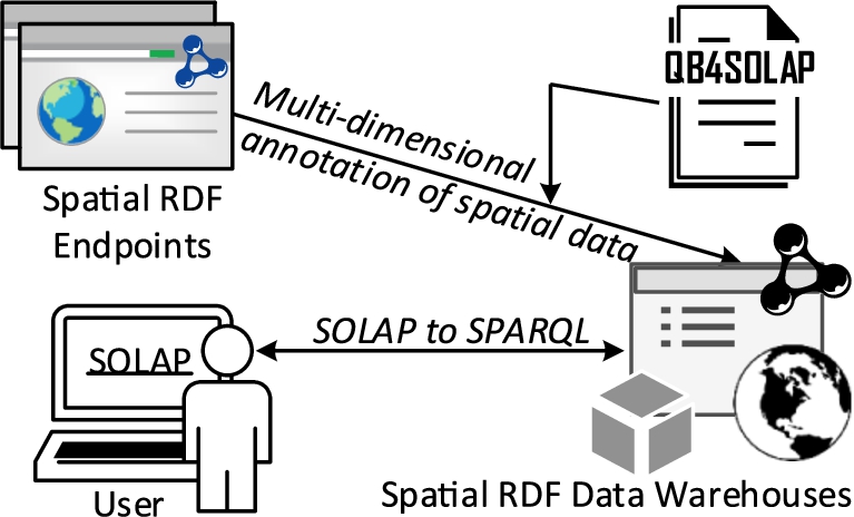
QB4SOLAP approach to SOLAP on the SW.
Similarly, providing deep spatial analytics support for spatial SW data is very valuable. Spatial data requires specific treatment techniques, in particular encoding, special functions and different manipulation methods, which should be considered in the modeling process and querying. The current state of the art for the geospatial Semantic Web focuses on techniques for publishing, linking and querying spatial data, but supports only “plain” spatial SW data (without support for spatial DW concepts such as spatial hierarchies, levels, and measures) and does not consider analytical queries over spatial RDF data (see Section 2 for details).
EuroStat:
UK Environmental Data:
Danish Agricultural Data: https://datahub.io/dataset/govagribus-denmark.
Australian Climate Observations:
DW and OLAP technologies have been successful for analyzing large volumes of data [1]. Combining DW/OLAP technologies with RDF data makes RDF data sources more easily available for interactive analysis. The following work concerns the integration of DW/OLAP with the SW.
Several conceptual models are proposed for representing spatial data in data warehouses. Stefanovic et al. [19] considers constructing and materializing spatial cubes in their proposed model. The MultiDim conceptual model, introduced by Malinowski and Zimányi [27], copes with spatial features and is extended in [36], to include complex geometric features (continuous fields), with a set of operations and an MD calculus supporting spatial data types. Gómez et al. [14] propose an algebra and a general framework for OLAP cube analysis on discrete and continuous spatial data. Even though spatial data warehousing is thus widely studied, those studies are limited to traditional non-semantic spatial data warehouses and SOLAP techniques. The work above neither considered semantic web data nor spatial analytical querying in SPARQL.
In summary, none of the related work, which is surveyed in the fields of “DW/OLAP and the SW”, “Spatial DW and OLAP”, and “Geospatial Semantic Web” provides a substantial foundation for modeling and querying spatial data warehouses on the Semantic Web, unlike the QB4SOLAP vocabulary, SOLAP operators, and SPARQL generation algorithms presented in this paper.
In this section, we describe the spatial objects and the spatial operations that manipulate them. Then, we introduce the data cubes and spatial enhancement on them as spatial data cubes. Finally, we show the traditional OLAP operations, which manipulate data cubes, and explain the Spatial OLAP (SOLAP) operators, which manipulate spatial data cubes.
Spatial objects
A spatial object represents a real-world object whose geographic features are important for an application. These geographic features are encoded using the geometry data type. Point, Line, and Polygon are the basic instantiable types of the geometry data type. Coordinates for geometry data type are generally given in 2-dimensions with X, Y values. Geometries are associated with a spatial reference system (SRS), which describes the coordinate space in which the geometry is defined. There are several SRSs and each of them are identified with a spatial reference system identifier (SRID). The World Geodetic System (WGS) is the most well-known SRS and the latest version is called WGS84, which is also used in our use case.
Spatial operations
There is a set of spatial operations that can be applied on spatial data. We grouped these operations into classes, based on the common functionality of the operators. These classes are defined next. The operators in the spatial aggregation class The operators in the topological relation class RCC8 (Region Connection Calculus) describes regions in Euclidean space or in a topological space by their possible relations to each other. DE-9DIM (Dimensionally Extended Nine-Intersection Model) is a topological model that describes spatial relations of two geometries in two dimensions. (Spatial aggregation).
(Topological relations).
The operators in the numeric operation class
Data cubes
Data warehouses store large volumes of data for decision support. They are based on the multidimensional model, which views data in an n-dimensional space, usually called a data cube. The cells of the cube represent the observation facts for analysis with a set of attributes called measures (e.g., a sales fact cube with measures product quantity and price). Facts are linked to dimensions, which provide perspectives to analyze data (e.g., sales date, product, and customer location). Dimensions are organized into hierarchies, which allow users to aggregate measures at various levels of detail. Hierarchies are composed of levels and there is always a unique top level All with just one member all. Levels have a set of attributes that describe the characteristics of the level members.
An example of a data cube with three dimensions (Customer, Time, and Product) and one measure (Quantity) is given in Fig. 2. Each cell in the cube is an observation fact, which is characterized by dimension and measure values. The hierarchies of this cube are given in Fig. 4(a)–(c). Thus, in the cube shown in Fig. 2, the Product dimension is given at the Category level, the Time dimension at the Quarter level, and the Customer dimension at the City level. Measure values represent the measure Quantity of the sold products.

A three-dimensional cube for Sales data.

Roll-up to the Country level.

Dimension hierarchies.
A spatial data cube contains both conventional and spatial dimensions. A spatial dimension is a dimension, which includes at least one spatial level in which the application should store the spatial characteristics of the members. Similarly, a hierarchy is a spatial hierarchy if it has at least one spatial level. Spatial characteristics of the levels are captured by their geometries and can be recorded in the spatial attributes of the level. A spatial fact is a fact that relates several dimensions in which, two or more are spatial.
For example, consider a Sales spatial fact, which has spatial dimensions Customer and Supplier, each with a spatial hierarchy Geography composed of spatial levels City → State → Country → All (Fig. 4(c)). These spatial levels record the spatial characteristics of its members with spatial attributes: Customer, Supplier, and City using a point spatial data type, whereas State and Country with a multi-polygon spatial data type.
Following the philosophy of spatially extended MultiDim conceptual model [36], MD concepts such as levels are considered to be spatial, only if they record the spatial characteristics of the concepts as geometries. For instance, “continent” might be considered as a spatial object, in theory or in other vocabularies. However, if there is no information about the geometry of the continents in the schema and in the instance data, continent does not become a spatial level (Extension 7), although continent might still be a traditional level (Definition 7) of the spatial hierarchy Geography with alphanumeric attributes (i.e., continent name, code, and etc.).
Spatial data cubes typically have spatial measures, which are also represented by a spatial data type. An example is a SalesPoint measure that stores the location of sales. Figure 7 shows the multidimensional schema of the GeoNorthwind data warehouse, which is used as running example in the paper.
OLAP operators
OLAP operators are used for expressing queries over data cubes. The traditional OLAP operators are given next.
The slice operator removes a dimension from a cube by selecting one instance in a dimension level. An example is “slice on City is equal to Odense”.
The dice operator selects the cells in a cube that satisfy a Boolean condition. An example is “dice on the first and last quarter of the year”.
The roll-up operator aggregates measures along a hierarchy to obtain data at a coarser granularity. An example is “roll-up to the Country level” (Fig. 3).
Finally, the drill-down operator disaggregates measures along a hierarchy to obtain data at a finer granularity. It is the inverse operation of roll-up. Starting from the cube in Fig. 3, an example is “drill-down to the City level”.
Spatial OLAP operators
Spatial OLAP (SOLAP) operates on spatial data cubes. SOLAP increases the analytical capabilities of OLAP by taking into account the spatial information in the cube. SOLAP operators involve spatial conditions or spatial functions by using the spatial operators defined in Section 3.1. Spatial conditions specify constraints on the geometries associated to cube members or measures, while spatial functions derive new data from the cube, which can be used, e.g., to derive dynamic spatial hierarchies or levels, as explained in the following example. Spatial extensions of the common OLAP operators are formally defined in Section 5.
Sample (instance) data for the Sales cube
Sample (instance) data for the Sales cube

Example map of Sales (instance) data.
Consider the summarized data for the Sales cube given in Table 1, where a ‘–’ is used if there are no sales to customers from the corresponding suppliers. The data in Table 1 is shown on the map in Fig. 5, where the arrows on the map between the supplier and customer locations represent the distance. The quantities of sold products are shown along these arrows.
The hierarchies in Fig. 4(a)–(c) can be used to perform classical roll-up operations, where measures are aggregated from a child to a parent level. An example of such a roll-up operator is expressed by the query “total sales to customers by city”, whose results is given in Table 2.
On the other hand, as shown in Table 4 and Fig. 5, some customers may be closer to suppliers from other cities. For example, customer c3 is related to its city Dortmund by using traditional Geography hierarchy, but the customer is closer to the city Düsseldorf of supplier s1. Similarly, customer c4 in city Dortmund is closer to the city Münster of supplier s3. Figure 4(d) shows a new dynamic spatial hierarchy that can be obtained with a spatial roll-up (s-roll-up) operator that expresses the query “total sales to customers by city of the closest supplier”. Such queries are not possible to express on conventional hierarchies with traditional OLAP.
The hierarchy in Fig. 4(d) is created on the fly with the help of a spatial function computing the distance between customer and supplier locations. Therefore, using the s-roll-up operator, sales to customers are aggregated by city of the closest suppliers, where Dortmund has a significant drop off in the quantity of the sales from 34 (Table 2) to 20 (Table 3).
Roll-up of the Sales cube
S-Roll-up of the Sales cube
Customer to Supplier distance
In this section, we formally define how to represent (spatial) data cubes in RDF. We use as running example the GeoNorthwind data warehouse whose conceptual schema is given in Fig. 7.

The QB4SOLAP vocabulary.
The QB4OLAP [11] vocabulary allows to define cube schemas and cube instances as RDF triples. QB4OLAP is an extension of the RDF Data Cube Vocabulary (QB) [5] with multidimensional concepts in order to be able to support OLAP operations directly over RDF data with SPARQL queries. We extended QB4OLAP (v1.2)8
with spatial concepts to give QB4SOLAP [16]. We based our extension on GeoSPARQL [30], a standard from the Open Geospatial Consortium (OGC) for representing and querying geospatial linked data for the Semantic Web. Since our base vocabulary QB4OLAP uses the MultiDim conceptual model to describe the multidimensional concepts, we base our definitions on a spatially extended version of MultiDim conceptual model [36] for spatial extension of the MD concepts. Fig. 6 shows the QB4SOLAP vocabulary for representing a spatial cube schema and spatial cube members as RDF triples. A cube schema defines the structure of the cube in terms of dimension levels, measures, aggregation functions (e.g., SUM, AVG, COUNT) on measures, spatial aggregation functions (Terms with capitalized initials and non-italic font in Fig. 6 represent RDF classes, terms with capitalized initials and italic font represent RDF instances, and terms with non-capitalized initials represent RDF properties. Classes in external vocabularies are depicted in light gray background and font. RDF Cube (QB), QB4OLAP, and QB4SOLAP classes are shown, respectively, with white, light gray, dark gray backgrounds. Original QB terms are prefixed with
RDF cube:
QB4OLAP:
QB4SOLAP:
GeoSPARQL:
In what follows, we first define formally RDF triples, and then discuss how to describe (spatial) multidimensional data using QB4OLAP and QB4SOLAP.
An RDF triple
A set of RDF triples is referred to as a graph. We denote a QB4SOLAP graph by
Given an MD element
Defining spatial data cube schemas with QB4SOLAP
An n-dimensional cube schema
We define next how to represent a cube schema
(Dimensions).
An n-dimensional cube schema
(Spatial dimensions).
A dimension is spatial if it has at least one spatial level. A spatial dimension

Conceptual multidimensional schema of the GeoNorthwind data warehouse.
The triples below show how some of the dimensions of the GeoNorthwind DW (Fig. 7) are represented in RDF using Definition 5 and Extension 5. As we will see below, the Customer and Supplier dimensions are spatial as they both have a spatial hierarchy Geography.

A dimension d has a set of hierarchies
(Spatial hierarchies).
A hierarchy is spatial if it contains at least one spatial level. A spatial hierarchy
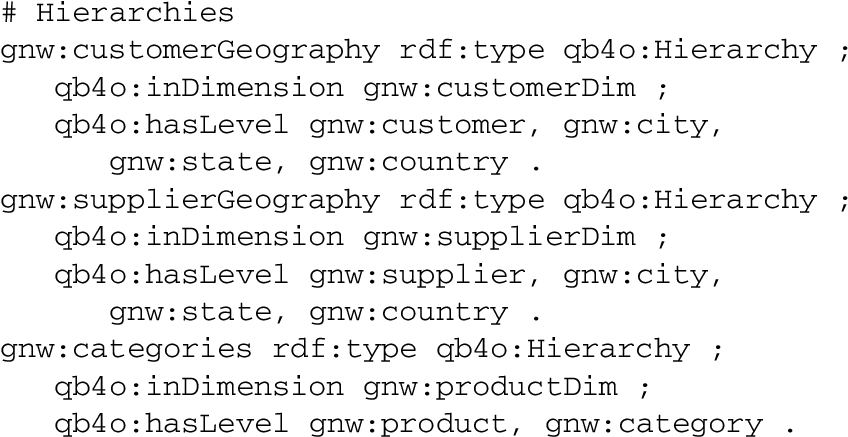
The triples below show how some of the hierarchies of the GeoNorthwind DW (Fig. 7) are represented in RDF using Definition 6 and Extension 6. As we will see below, the Geography hierarchies in the Customer and Supplier dimensions are spatial since they have spatial levels (City, State, etc.)
A hierarchy h has a set of levels
(Spatial levels).
A level is spatial if it has an associated geometry. A spatial level
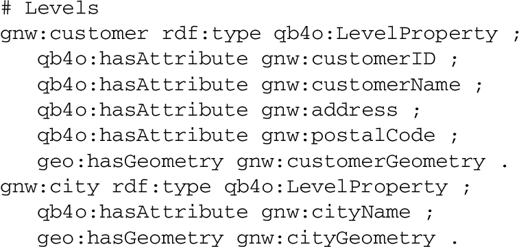
The triples below show how some of the levels of the GeoNorthwind DW (Fig. 7) are represented in RDF using Definition 7 and Extension 7. Note that the Customer and City levels are spatial as they have a geometry that is specified at the level definition.
A level l has a set of attributes
(Spatial attributes).
An attribute is spatial if it is defined over a spatial domain. A spatial attribute
The triples below show how some of the attributes of the GeoNorthwind DW (Fig. 7) are represented in RDF using Definition 8 and Extension 8. Note that the Customer level has a spatial attribute (Customer geometry). It is represented as a WKT literal that defines a Point type from the Geometry class, which is a subclass of Spatial Object.

A hierarchy h has a set of hierarchy steps
Each hierarchy step
(Spatial hierarchy steps).
A hierarchy step is spatial if it relates a spatial child level
The triples below show how the hierarchy steps of the Geography spatial hierarchy in the Customer dimension of the GeoNorthwind DW (Fig. 7) are represented in RDF using Definition 9 and Extension 9. Note that all hierarchy steps are spatial and have an associated topological relation.

The hierarchy steps
(Measures).
An n-dimensional cube schema has a set of measures
(Spatial measures).
A measure is spatial if it is defined over a spatial domain as in spatial attributes (Extension 8). A spatial measure
The triples below show how the measures of the GeoNorthwind DW (Fig. 7) are represented in RDF using Definition 11 and Extension 11. Note that SalesPoint is a spatial measure, which records the location of the stores in which the sales occurred. It is defined over Geometry domain as a Point type with WKT literal.

In an n-dimensional cube schema
(Spatial fact).
A fact is spatial if it relates several levels, where two or more are spatial. A spatial fact may also have a topological relation
The triples below show how the fact of the GeoNorthwind DW (Fig. 7) is represented in RDF using Definition 12. Sales fact does not impose any topological relation between its spatial dimensions Supplier and Customer. SalesPoint is a spatial measure, which has a spatial aggregate function (AggrConvexHull).

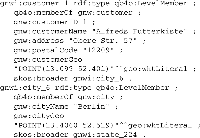
We have explained in Section 4.1 how a data cube schema can be represented in RDF with QB4SOLAP. We show next how to use this schema to represent the instances of the GeoNorthwind DW (Fig. 7) in RDF. We denote by A level l has a set of level members A level member A hierarchy step The triples below show how some level members of the GeoNorthwind DW (Fig. 7) are represented in RDF using Definitions 13–14.
A fact F has a set of fact members A fact member The triples below show how a fact member of the GeoNorthwind DW (Fig. 7) is represented in RDF using Definitions 12–16. Note that the fact member and corresponding level members relating to dimensions are given with the prefix
(Level members).
(Attributes of level members).
(Partial order on level members).

This section defines a formal algebra for SOLAP operators. Examples of the operators are provided after their definitions. The complete SPARQL query examples are given at our website13
The slice operator removes a dimension from a cube
(S-Slice).
The s-slice operator removes a dimension from a cube
As for the semantics, s-slice takes an n-dimensional cube
The operator is defined as:
The s-slice operator selects a subset
To sum up, the subset
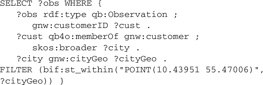
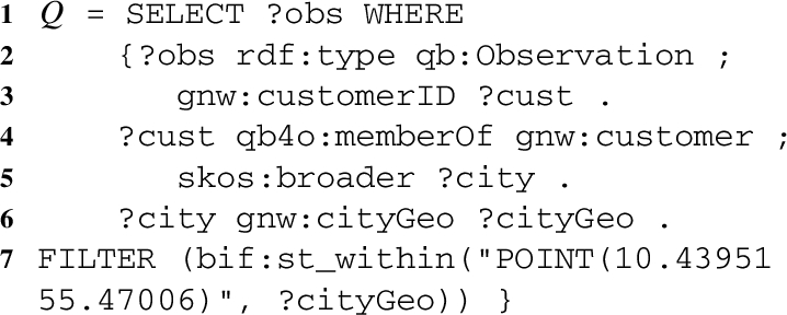
With regards to the traditional slice query “slice on customers in the city of Odense”, in s-slice, the user could specify a geometry extent (e.g., polygon coordinates of the city of Odense) as spatial literal for slicing instead of giving a text literal (e.g., “Odense”). So the s-slice query would be; “slice on customers of the city, which has the geometry The following SPARQL query shows an s-slice operator, which filters with the given spatial literal by the user. The following SPARQL query shows the s-slice operator, which filters with the function call (largest city) returned from inner select. Given the current limitations of SPARQL, there is not an area calculation function from the geometries of the spatial objects during query run time, however we give the query with a notional built-in 

With regards to the traditional slice query “slice on customers in the city of Odense”, in this example of s-slice, the user gives a point geometry (i.e.,
The following SPARQL query shows an s-slice operator, which filters at the specified level with the given spatial literal by the user.
Note that the s-slice can be operated in different ways based on the geometry given to the query. In both Examples 11 and 12, slice level is given as City, however in Example 12 a random
The traditional dice operator takes a cube and a Boolean condition ϕ, which returns a new cube containing only the cells that satisfy the Boolean condition ϕ. Dice operation is analogous to relational algebra, R selection;
(S-Dice).
Similarly, the s-dice operator takes an n-dimensional cube
The semantics of the operator is defined as:
The s-dice operator selects a subset Spatial predicate on level values: Spatial predicate on level attribute values: Note that the filtering the facts through level members can be done by Spatial predicate on measure values of
For complex cases, i.e., combining these three types; the result set is also followed by combining the basic result sets.
The s-dice operator can be implemented on level and attribute values by filtering level members in the cube or on measures by filtering the facts in the cube. In both cases the spatial predicate
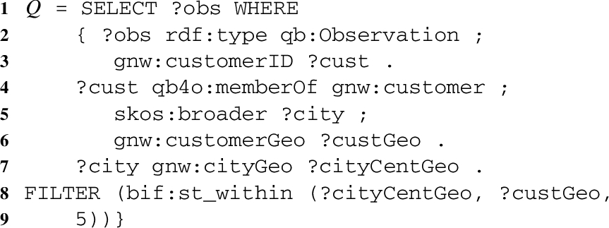
The query for the s-dice operator could be “sales to customers, which are located within 5 km distance from their city center” where the s-dice is on level members by filtering the customer level. The spatial predicate First method is assuming a buffer area of 5 km from the coordinates of city center and checking customers’ locations by within operator from topological relations Second method is checking if the distance from a customer location to the corresponding city center is less than 5 km, by using distance function from numeric operations 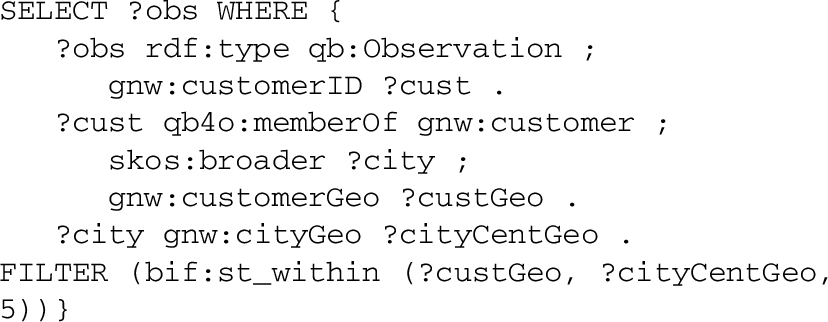

The traditional roll-up operator aggregates measures according to a dimension hierarchy (by using an aggregate function), in order to obtain measures at a coarser granularity for a given dimension. For example, the query “total amount of sales to customers by city” is a classical roll-up operation. (Cube is the sales, dimension is the customer, level in dimension to roll-up is the city such that
(S-Roll-up).
Similarly to roll-up operator, s-roll-up aggregates measures
As for the semantics, s-roll-up takes an n-dimensional cube
The set of level members of the level
The extension to multiple measures is similar, which is done by providing and using a separate aggregate function for each measure
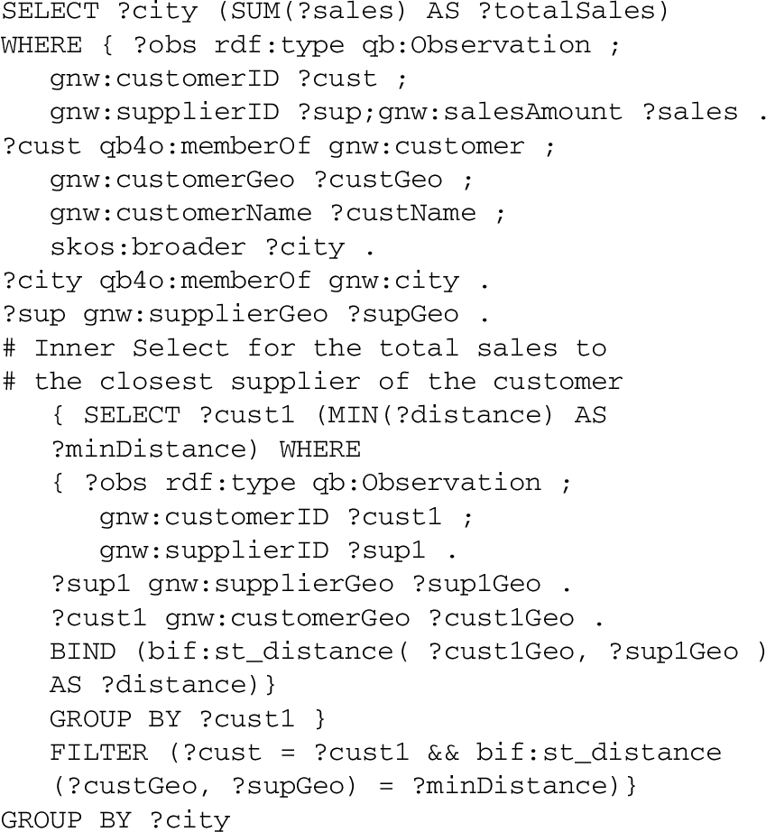
The following SPARQL query shows the s-roll-up operator, which is exemplified in Section 3.6. The query is “total amount of sales to customers by city of the closest suppliers”. Note that the measures are aggregated up to a new city from customer level of the customer dimension, which is specified as the Closest City. The hierarchy step from customer to city is defined dynamically by a spatial function
Drill-down is the inverse operator of roll-up, which disaggregates previously summarized data to a child level in order to obtain measures at a finer granularity of a given dimension. For example, the roll-up query given in Remark 19 (“total amount of sales to customers by city”) aggregates sales by summing up the sales amount, from customer level to city level along a hierarchy. As drill-down operator performs the operation opposite to the roll-up an example would be; “average amount of sales of each supplier, drilled down from the city level to the supplier level”. (Cube is the same as sales, and the hierarchy is the same but the dimension is the supplier, so child level in dimension to drill-down from city level is the supplier such that
(S-Drill-down).
Analogously to drill-down operator, s-drill-down disaggregates measures
Conceptually, in s-drill-down, the dimension hierarchy is created dynamically on levels by the spatial function
In order to exemplify an s-drill-down, starting from the result cube graph of Example 14 (“total amount of sales to customers by city of the closest supplier”), which is at the granularity of City level, we drill down to child level Supplier with the query “average amount of sales of furthest suppliers to their city center, drilled down the from City level to Supplier level”. The following SPARQL query shows the given example.

In this paper, we focus on direct querying of single data cubes with main SOLAP operators in SPARQL. The integration of several cubes through s-drill-across or set-oriented operations such as union, intersection, and difference [7] is out of scope and remained as future work.
After having defined the high-level SOLAP operators in Section 5, this section first describes how to generate SPARQL queries for each of these operators by using the QB4SOLAP metamodel (Section 4). Afterwards, this section describes how to create more complex SPARQL queries for nested SOLAP operations.
Generation algorithms
The generated SPARQL queries Q are of the form “
RDF datasets published with the QB4SOLAP vocabulary use the
Thus, we define a helper function

In order to represent such varying parameters at the instance level such as fact members, level members, or parameter values given by the user, and to distinguish these parameters from other parameters in the algorithm, we represent such parameters using variable names with question marks.
We use a
We apply them on measure values or use them as wrappers in spatial functions. In the following, we often write
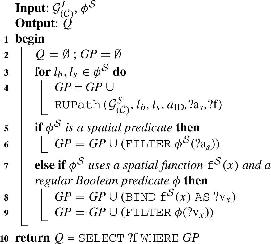
In the following, we present the SPARQL query generation algorithms for the SOLAP operators defined in Section 5. The algorithms take the input parameters and arguments of the SOLAP operator and return the a SPARQL query Q that can be executed.
On the other hand the given spatial literal in Example 12 has the geometry data type point, which corresponds to the spatial level
Get the path for dimension

Check if the spatial literal
Build the FILTER statement based on the spatial literal

Check if
Call the

Build a bind statement on

Generate the inner select query

Build the filter statement with the output of the spatial function

If a spatial literal

Finally, the algorithm generates query Q, which can be executed over the fact members
S-Slice operator with a given spatial value as point data type: The following listing corresponds to the SPARQL output of the running example where the spatial value is given as
S-Slice operator with a spatial function call: The following listing corresponds to the SPARQL output of the running example where the spatial value is returned from a function call (Example 11.2). The graph pattern

S-Slice operator with a given spatial value as polygon data type: The following listing corresponds to the SPARQL output of the running example where the spatial value is given as a

“sales to customers, which are located 5 km distance from their city center”. In the following, we discuss the main steps of Algorithm 3 with the running example, where the steps are referencing the line numbers in Algorithm 3.
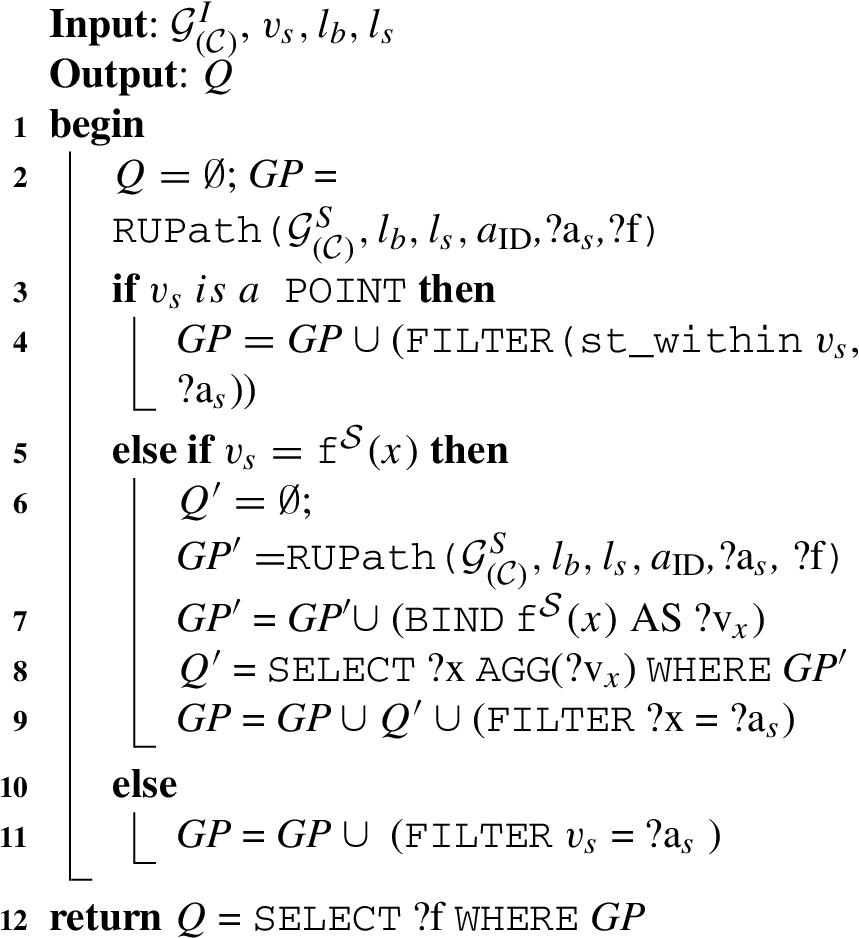
The algorithm runs through the levels from base level
Build the roll-up path for those levels using the helper function

Check if
Create a filter statement with a spatial predicate and the spatial level attribute

Check if
Create a bind statement based on a spatial function (i.e., calculate

Generate query Q for selecting the facts
S-Dice operator with
S-Dice operator with

Build the roll-up path using helper function
Build inner select subquery to apply the spatial function
Call
Build the bind statement in order to calculate the spatial function
Generate the inner select query
Build the filter statement for the whole query based on the output of the spatial function, which is calculated in the inner select subquery. Then, add the filter and inner select subquery to the main graph pattern Generate query Q for computing the facts
S-Roll-up operator: The following listing shows the generated SPARQL query. Graph pattern 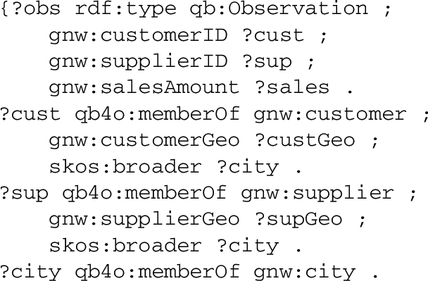


 Note that in Line 9, the spatial target level

We now show how a SPARQL query can be generated for a nested SOLAP expression. In general, a nested set of SOLAP operators can be rewritten into an expression with an additional s-dice, on top of a series of s-roll-ups, on top of one or more s-slices, on top of an s-dice, i.e., (s-dice
Let us begin with a simpler nested form that shows the most typical pattern, namely (s-roll-up (s-slice (s-dice(
We formulate the nested SOLAP query as
Principle 1: Perform s-dice in the beginning or at the end.
Principle 2: If there are several s-roll-up or s-slice operations call their generator algorithms repeatedly.
Principle 3: Always separate
Principle 4: Build the final graph pattern with the separated and enumerated
Principle 5: Drop the main
Principle 6: Separate the

To separate the

The graph pattern
Conclusions and future work
Motivated by the need for a formal foundation for spatial data warehouses on the Semantic Web, this paper made a number of contributions. First, it proposed the QB4SOLAP vocabulary (metamodel), which supports spatially enhanced multidimensional (MD) data cubes over RDF data. This allows users to publish MD spatial data in RDF format. Second, the paper defines a number of spatial OLAP (SOLAP) operators over the defined QB4SOLAP cubes, allowing spatial analytical queries over RDF data, and gives their formal semantics. Third, the paper provides algorithms for generating spatially extended SPARQL queries from individual and nested SOLAP operators, allowing users to write their spatial analytical queries in our high-level SOLAP language instead of the lower-level and more complex SPARQL. Fourth, the vocabulary, operators, and query generation algorithms are validated by applying them to a realistic use case.

Our future vision of SOLAP on the SW.
Figure 8 presents our future vision of SOLAP on the Semantic Web with regards to the current state of the art and ongoing work. In order to verify the algorithms, which are defined in this paper, we developed GeoSemOLAP [18], a SPARQL query generation tool. GeoSemOLAP allows users to perform SOLAP operations and generate SPARQL queries interactively through a GUI. We refer to our screencast16
Publishing spatial DWs on the SW allows users to also exploit the existing external geo-vocabularies (e.g., GeoNames, etc.)17
GeoNames:
Additional interesting aspects of future work would be, for instance, extending the formal techniques and algorithms for generating SOLAP queries in SPARQL to work over multiple RDF cubes, i.e., to support s-drill-across, and supporting spatial aggregation (s-aggregation) with user-defined functions over spatial measures. It would be also interesting to increase efficiency by extending our spatial data warehouse with techniques that been developed in the context of RDF data cubes and SPARQL analytical queries in general, e.g., materialization and optimizing the physical layout [13,21,22], and to enable efficient support of a broad range of external sources by considering aspects such as federated processing of analytical queries [20] and schema heterogeneity [34]. We will also consider more efficient representations of the data, e.g., by removing redundancies. Furthermore, it would be interesting to extend QB4SOLAP and GeoSemOLAP [18] to handle highly dynamic spatio-temporal data and queries, as for instance, found in large-scale transport analytics [12].
Footnotes
Acknowledgement
This research is partially funded by the European Commission through the Erasmus Mundus Joint Doctorate Information Technologies for Business Intelligence (EM IT4BI-DC) and the Danish Council for Independent Research (DFF) under grant agreement no. DFF-4093-00301.