Sage Journals: Discover world-class research

Abstract

Due to the advantages of flame cutting in thick plate cutting and cutting cost, it is widely used in the metal cutting process of shipbuilding and machinery manufacturing. But at the same time, the local heating of flame cutting will cause residual stress inside the steel plate. Residual stress is an important reason for deformation and cracking of components. The change of temperature field is the premise of affecting the distribution of residual stress. Cutting speed has an important effect on the distribution of temperature field and residual stress field. In this paper, ABAQUS is used to create a finite element model for flat flame cutting of Q345D low-alloy steel. Based on the working principle of flame cutting, the model of flame cutting composite heat source is established and the subprogram of composite heat source is written. The thermal-mechanical direct coupling method is used to simulate and analyze the effect of different cutting speeds on the temperature and residual stress field distribution of the flat flame cutting process, to provide a reference for the subsequent processing.

Keywords

Flame cutting numerical simulation cutting speed temperature field residual stress

1. Introduction

The flame cutting process is an indispensable metal cutting method in shipbuilding and machinery manufacturing. In recent years, plasma and laser cutting technologies have gradually matured, and have gradually replaced flame cutting in medium and low thickness metal cutting, but flame cutting is still widely used in shipbuilding and heavy machinery manufacturing because of its advantages of simple equipment, convenient operation, suitable for thick plate cutting and low equipment cost. Flame cutting has many similarities to welding, but is more complicated than welding. During flame cutting, the kerf position will be heated briefly and rapidly by high-density heat flow, causing a large temperature difference between the kerf position and the base material. After cutting, the metal surface temperature drops rapidly, this uneven the heating and cooling methods cause incongruous strains in the interior of the metal being cut, which creates residual stress. During the subsequent welding process is performed, the residual stress generated by cutting will be redistributed under the action of the welding heat, and then superimposed with the residual stress field generated by the welding heat source itself, finally forming a cutting and welding coupling residual stress field, which makes the research on welding more difficult and affects the bearing capacity and structural strength of the welded workpiece. The initial stress caused by it cannot accurately simulate the actual situation.

At present, there have been some researches on the numerical simulation of thermal cutting at home and abroad. Kim et al. [1] proposed a transient two-dimensional model of high-energy laser cutting metal, derived the dimensionless form and boundary conditions of the governing equation, and analyzed the performance of material removal under different parameters; Arif et al. [2] modeled the laser cutting of thick low-carbon steel plate, and used XDR technology to study the residual stress value of the cutting position, and compared it with the predicted value; Yilbas et al. [3]modeled the thermal stress generated by the laser cutting edge, analyzed the temperature field and stress field, and verified it through experiments; Jiao et al. [4] proposed a method of processing glass with dual CO2 laser beams, used ANSYS to study the temperature and stress distribution, and studied the thermal stress during single and double laser beam processing; Kheloufi et al. [5] established a three-dimensional transient numerical model to study the temperature field and incision shape of the laser melting process; Zhou et al. [6] based on the energy balance of oxygen cutting, through the study of the interaction between the Gaussian region heat source and the heat generating heat source, a new type of oxygen cutting composite heat source model was created, and the finite element analysis of oxygen cutting was carried out in combination with the life-death unit, and the model was verified by experiments; Bae et al. [7] the heat source modeling was carried out on the oxygen-ethylene flame-cut steel plate, performed numerical simulations on the heat flow in the steel plates, and verified the feasibility of the heat source by comparing the heat-affected zones calculated by experiments and numerical simulations; Thiébaud et al. [8] measured the temperature and heat-affected zone during flame cutting of thick steel plates, established a three-dimensional model of flame cutting, and improved the model according to the measured values; Huang et al. [9] conducted cutting residual stress analysis on PEC wall webs with holes and without holes, and conducted welding residual stress research on whether to input cutting residual stress as a condition, and finally obtained the residual stress distribution of the two kinds of webs; Jokiaho et al. [10] used ABAQUS to model and simulate the process of flame cutting heavy steel plates, obtained the temperature and residual stress during the cutting process, and verified the established model through experiments; Arenas et al. [11] described a model for the study of heat distribution and solid-liquid phase transition during flame cutting of steel plates, and verified it through experiments; Lindgren et al. [12] established a calculation model for flame cutting simulation, and compared the residual stress under room temperature and preheating conditions; Moradi et al. [13] simulated the laser cutting of 3.2 mm thick polycarbonate sheet, and studied the influence of laser power, cutting speed and other process parameters on the width of the kerf and the heat-affected zone; Peirovi et al. [14] modeled and simulated laser cutting of 1.2 mm thick aluminum sheet, predicted the temperature field and stress field distribution and heat-affected zone during the cutting process, and verified the effectiveness of finite element simulation of laser cutting; Sharifi et al. [15] conducted numerical simulations on laser cutting LL6061T6 alloys, and studied the effects of parameters such as cutting speed, laser power, and sheet thickness on the cutting temperature field and cutting quality; Xiong et al. [16] established a mathematical model of the cutting heat source, and predicted the temperature field of the U-rib and the diaphragm thermally cut welded joint. A numerical elastoplastic thermomechanical model for predicting the evolution of residual stresses in diaphragm-rib joints throughout the fabrication process including flame cutting and welding was developed and validated experimentally.

At present, in terms of thermal cutting simulation research, the research is mainly on the temperature field distribution of laser cutting or flame cutting thin plates, and there are few simulation studies on flame cutting residual stress. When studying the cutting temperature field and residual stress, the indirect coupling method is often used. Compared with the thermal direct coupling, the thermal indirect coupling has complicated steps and low calculation accuracy. The heat source models used include Gaussian surface heat source plus heat generation, cylindrical heat source and so on. The modeling in this paper is based on the working principle of flame cutting, and a cutting composite heat source model is established, and the thermal-mechanical direct coupling is used instead of the traditional indirect coupling method to simulate the temperature field and residual stress field distribution of flame cutting at different cutting speeds. Provide reference for welding and other processing.

2. Flame cutting process theory

2.1 The principle of flame cutting

As shown in Fig. 1, when the cutting starts, the surface of the workpiece first reaches the ignition point under the action of the preheating flame, which is a mixture of high-purity oxygen and cutting gas. Then a high-purity, high-pressure cutting oxygen flow is introduced, so that the iron in the preheated workpiece burns in the cutting oxygen to produce oxide slag, and at the same time generates a large amount of heat. The combustion heat continues to heat the lower layer of the workpiece and the edge of the cut, making the metal reach the ignition point or even melt, and the generated oxide slag is blown away from the workpiece by the cutting oxygen flow, the preheating flame and the cutting oxygen flow move at a constant speed to form a kerf, and finally the workpiece is cut. That is to say, the whole cutting process is divided into three stages:

(1)
In the preheating stage, the preheating flame heats the surface metal at the cutting point of the workpiece to the ignition point;
(2)
In the combustion stage, the surface metal of the workpiece undergoes a violent oxidation reaction with high-purity cutting oxygen, and extends to the lower metal;
(3)
In the slag blowing stage, the high-speed cutting oxygen flow blows away the generated iron oxide slag to form a kerf, and the preheating flame continues to heat the metal on the upper surface of the kerf to the ignition point, and the cutting oxygen moves forward at a uniform speed to form continuous cutting.

Figure 1.
Schematic diagram of flame cutting.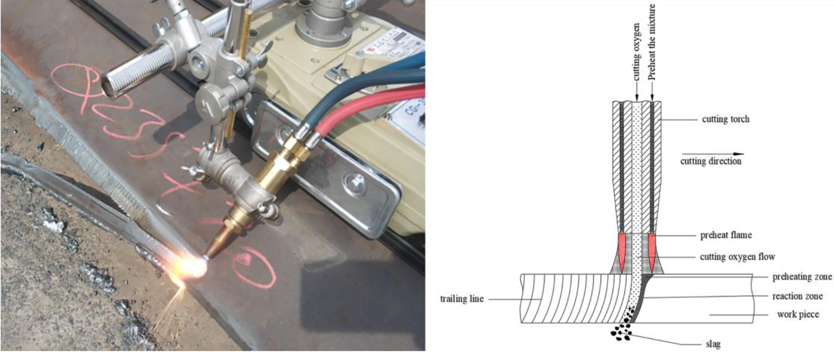

2.2 Heat conduction governing equations and boundary conditions

(1) Flame cutting is a three-dimensional transient nonlinear heat conduction problem, so the governing equation of heat conduction is expressed as:

$\displaystyle\rho c\frac{\partial T}{\partial t}=\frac{\partial}{\partial x}% \left({\lambda\frac{\partial T}{\partial x}}\right)+\frac{\partial}{\partial y% }\left({\lambda\frac{\partial T}{\partial y}}\right)+\frac{\partial}{\partial z% }\left({\lambda\frac{\partial T}{\partial z}}\right)+\frac{\partial Q}{% \partial t}$ (1)

Where: $\rho$ is the material density, kg/m³; $c$ is the specific heat, J/(kg $\cdot{}^{\circ}$ C); $\lambda$ is the thermal conductivity, W/(m^{2 ⋅^∘}C); $T$ is the temperature, ^∘C; $t$ is the time, $s$ ; $Q$ is the heat source intensity, J/m³.

(2) Thermal boundary conditions during flame cutting:

The temperature distribution is a function $T$ of the three-dimensional space coordinates with respect to time, and the temperature distribution at the initial $t=$ 0 is:

$\displaystyle T_{0}=T\left({x,y,z,0}\right)$ (2)

The first type of boundary condition is that the temperature on the boundary is known:

$\displaystyle T_{s}=T_{s}\left({x,y,z,t}\right)$ (3)

The second type of boundary condition is that the heat flux on the boundary is known:

$\displaystyle\lambda\frac{\partial T}{\partial n}=Q_{s}\left({x,y,z,t}\right)$ (4)

The third type of boundary condition is that the heat exchange on the boundary is known:

$\displaystyle\lambda\frac{\partial T}{\partial n}=\alpha\left({T_{\alpha}-T_{s% }}\right)$ (5)

2.3 Basic theory of cutting temperature field calculation

The flame cutting process is a transient heat transfer process, and the finite element solution of heat transfer is expressed as:

$\displaystyle\left[{C\left(T\right)}\right]\mathop{\left\{T\right\}}\limits^{% \cdot}+\left[{K\left(T\right)}\right]\left\{T\right\}=\left[{Q\left(T\right)}\right]$ (6)

Where: $\left[{C\left(T\right)}\right]$ is the heat capacity matrix; $\left[{K\left(T\right)}\right]$ is the thermal conductivity matrix; $\left\{T\right\}$ is the nodal temperature vector; $\{\dot{T}\}$ is the temperature-time derivative; $\left[{Q\left(T\right)}\right]$ is the nodal heat flow rate vector.

2.4 Flame cutting stress-strain theory

The cutting stress and strain are based on the heat conduction analysis. It is assumed that the material yield obeys the Von Mises yield criterion, and the plastic flow criterion and strengthening criterion are obeyed in the plastic zone. The stress-strain constitutive equation is expressed as:

$\displaystyle\left\{{d\sigma}\right\}=\left\{D\right\}\left\{{d\varepsilon}% \right\}-\left\{C\right\}dT$ (7)

Where: $\left\{{d\sigma}\right\}$ is the stress increment; $\left\{{d\varepsilon}\right\}$ is the strain increment; $\left\{D\right\}$ is the elastic or elastoplastic matrix; $\left\{C\right\}$ is the temperature-related vector.

3. Q345D flame cutting finite element model establishment

3.1 Numerical simulation method of flame cutting

The flame cutting temperature field is a transient temperature field formed by the preheating flame and the iron-oxygen combustion reaction. ABAQUS software is used to simulate the thermal-mechanical coupling process of flat flame cutting. The thermal-mechanical coupling includes direct coupling and indirect coupling (sequence coupling) in two ways. At present, most thermomechanical coupling studies use indirect coupling methods, but the direct coupling method has stronger coupling degree and easier operation, as shown in Table 1. Therefore, this paper uses thermal-mechanical direct coupling method for numerical simulation in the analysis of flame cutting temperature field and residual stress.

Table 1
Comparison of direct coupling and indirect coupling

Coupling method	Direct coupling	Indirect coupling
Degree of coupling	Higher	Lower
Calculation accuracy	Higher	Lower
Computational efficiency	Lower	Higher
Solving order	Simultaneously solve	Sequential solution
Unit type	Coupling unit	Thermal and Structural Units

3.2 Flame cutting finite element model

ABAQUS is used to establish flat linear flame cutting model and carry out grid division. The size of the finite element model is 150 mm $\times$ 120 mm $\times$ 10 mm, and the kerf width is 2 mm. Considering the heat source loading position and the accuracy of numerical simulation, the non-uniform grid division method is adopted, and the grid division in the kerf and the area near the kerf is relatively dense, with a size of 0.5 mm. The grid division in the edge area is relatively sparse, the grid unit type is temperature-displacement coupling unit C3D8T, the total number of units is 13440, and the total number of nodes is 17415. The cutting model size and grid division are shown in Fig. 2.

Figure 2.

Model size and mesh division.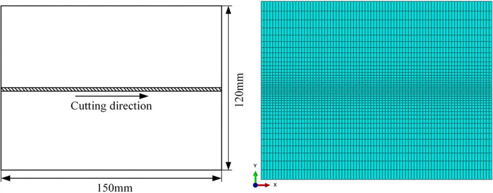

The cutting material is Q345D low-alloy steel commonly used in mechanical equipment manufacturing, with a yield strength of 345 MPa at room temperature. The material composition is shown in Table 2. During the thermal-mechanical coupling calculation process of flame cutting, some material parameters change with temperature. The high-temperature thermophysical properties of materials are difficult to determine, so some material properties are calculated using linear interpolation, as shown in Fig. 3. In order to better simulate the material removal process of flame cutting, it is necessary to use the Model change function to delete the cells that reach the melting point (1500^∘C) in the grid of the kerf area where the composite heat source passes.

Table 2

Chemical composition of Q345D steel material

Model Specifications	C	Mn	Si	P	v	Al	S	Fe
Q345D	0.164	1.360	0.370	0.015	0.025	0.028	0.011	Margin

Figure 3.

Q345D thermophysical properties.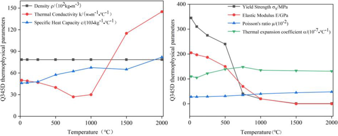

3.3 Establishment of composite heat source model

Flame cutting is an extremely complex and highly nonlinear process. The cutting process contains too many variables, which makes it difficult to verify and establish a heat source model. Therefore, it is necessary to simplify the flame cutting model. It can be seen from the actual flame cutting process that the heat generated is composed of two parts: preheating flame and iron-oxygen combustion reaction. In this paper, the preheating flame is a mixture of propane and preheating oxygen. Current research shows that the heat provided by the preheating flame is far less than the heat provided by the iron-oxygen combustion reaction, and the specific gravity of the heat provided by the iron-oxygen combustion reaction is positively correlated with the thickness of the model.

When flame cutting is performed, the metal is cut at a constant speed by the combined action of the preheating flame and the iron-oxygen combustion reaction to form a kerf, which is equivalent to the interaction of two different types of heat source models. There is still no clear definition of the flame cutting heat source model. Some studies consider the influence of the preheating flame, while others ignore the influence of the preheating flame. From the current research, the heat source model can be divided into several types, such as quasi-steady state model, heat generation rate model, Gaussian heat source model, and cylinder model. As shown in Fig. 4, this paper tries to establish a new cutting composite heat source model, the preheating flame acting on the metal surface is regarded as a moving Gaussian surface heat source acting on a semi-infinite body, and the burning of iron at the kerf is regarded as a rectangular heat source whose width is equal to the width of the kerf. To enhance the accuracy of the cutting process simulation, the length of the rectangular heat source is set to be equal to the length of the kerf cut per second.

Figure 4.

Model diagram of composite heat source.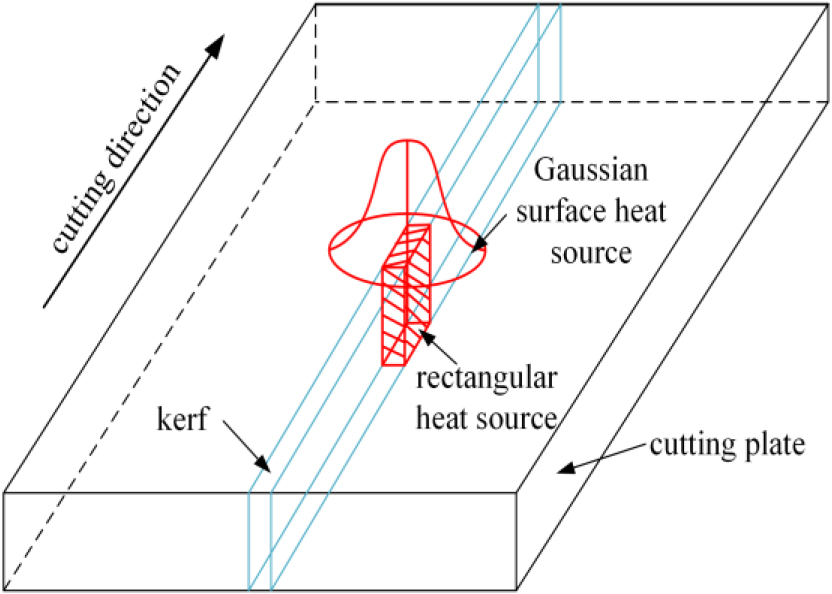

The preheating flame is a Gaussian surface heat source model, and its heat flux distribution curve is shown in Fig. 5.

Figure 5.

Gaussian heat flux curve.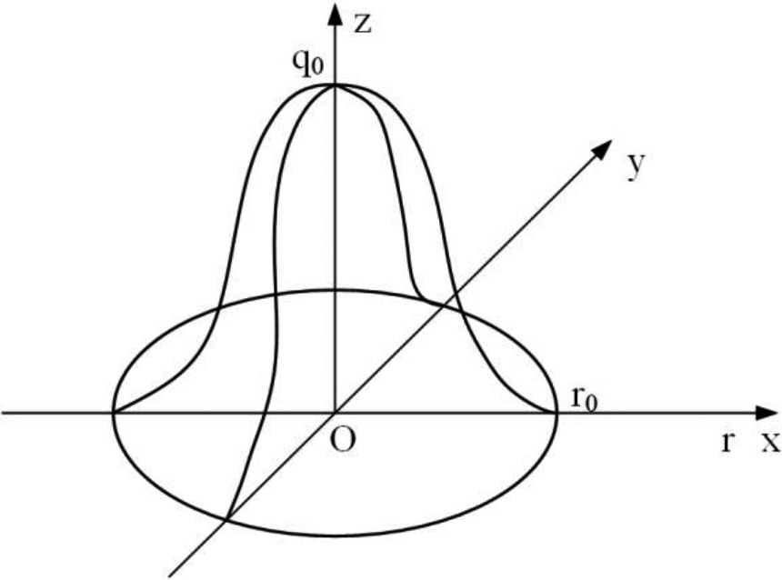

The heat flux expression is:

$\displaystyle q_{\left(r\right)}=q_{0}\exp\left({-Kr^{2}}\right)$ (8) $\displaystyle q_{0}=\eta_{\textit{pre}}\cdot Q_{C_{3}H_{8}}\cdot A_{C_{3}H_{8}% }\cdot K/\pi$ (9)

In summary:

$\displaystyle q_{\left(r\right)}=\frac{3\eta_{\textit{pre}}Q_{C_{3}H_{8}}A_{C_% {3}H_{8}}}{\pi r_{0}^{2}}e^{\left({\frac{-3r^{2}}{r_{0}^{2}}}\right)}$ (10)

Where: $q_{(r)}$ is the heat flow at $r$ from the center of the preheating flame is the heat flux density from the center of the heat source, $W/m^{2}$ ; $q_{0}$ is the maximum heat flux density at the center of the preheating flame, $W/m^{2}$ ; $K$ is the heat flux concentration coefficient, $K=3/r_{0}^{2}$ ; $r_{0}$ is the effective radius of the preheating flame, take $r_{0}=$ 0.035 m; $Q_{C_{3}H_{8}}$ is the propane flow rate, $m^{3}/s$ ; $A_{C_{3}H_{8}}$ is the calorific value of propane combustion, $J/m^{3}$ ; $\eta_{\textit{pre}}$ is the thermal efficiency of the preheating flame, usually take 0.2–0.35.

Three forms of metal iron-oxygen combustion reaction at the kerf:

$\displaystyle\textit{Fe}+0.5O_{2}\Rightarrow\textit{FeO}+267.8\textit{kJ}$ $\displaystyle\textit{2Fe}+1.5O_{2}\Rightarrow\textit{Fe}_{2}O_{3}+823.2\textit% {kJ}$ (11) $\displaystyle\textit{3Fe}+2O_{2}\Rightarrow\textit{Fe}_{3}O_{4}+1120.5\textit{kJ}$

It can be seen from the above reaction equation that the iron-oxygen combustion reaction generates FeO, $\textit{Fe}_{2}O_{3}$ and $\textit{Fe}_{3}\textit{O}_{4}$ three oxides, and the heat release of the three oxides is also different. The generated oxides also change with the different proportions of the plate thickness. According to the composition analysis of the 10 mm thick carbon steel gas cutting slag, the mass fractions of the three oxide slags generated by combustion are 20%, 55% and 25%, respectively, as shown in Table 3. According to the heat release of each oxide formed, the heat generated by the combustion of iron per unit volume can be calculated as $Q_{\textit{gen}}=5.035e^{10}(J/m^{3})$ .

Table 3

The heat release of oxides generated by iron-oxygen combustion reaction

Oxide	The heat of combustion of 1 g of iron (J)	The heat of combustion of 1 cm³ iron (J)	Quality score (w/%)
FeO	4.78 $\times$ 10³	3.76 $\times$ 10⁴	20%
Fe₂O₃	7.37 $\times$ 10³	5.801 $\times$ 10⁴	55%
Fe₃O₄	6.69 $\times$ 10³	5.265 $\times$ 10⁴	25%

In order to simulate the continuous flame cutting process, the moving Gaussian heat source and the iron-oxygen combustion reaction rectangular heat source are continuously loaded, and the thermal efficiency of the iron-oxygen combustion reaction needs to be considered.

4. Simulation result analysis

4.1 Analysis of cutting temperature field simulation results

Combined with the model material and size, the cutting speed is determined as $v=$ 5 mm/s, $v=$ 6 mm/s, $v=$ 8 mm/s, $v=$ 10 mm/s four situations respectively. Cutting residual stress is generated by uneven heating during cutting, so the temperature field at different cutting speeds should be analyzed first. When studying the temperature distribution characteristics of the flame cutting model surface, it is necessary to select a series of temperature data points on the model. Figure 6 shows the positions of the selected temperature data points, combined with the size of the cutting model, select 5 temperature data points along the kerf direction, select 5 temperature data points on the plane perpendicular to the kerf direction in the middle of the cutting model, and select 3 temperature data points on the middle section of the model along the kerf depth direction, and analyze the thermal cycle data of each temperature data point.

Figure 6.

Distribution of temperature data points of the cutting model.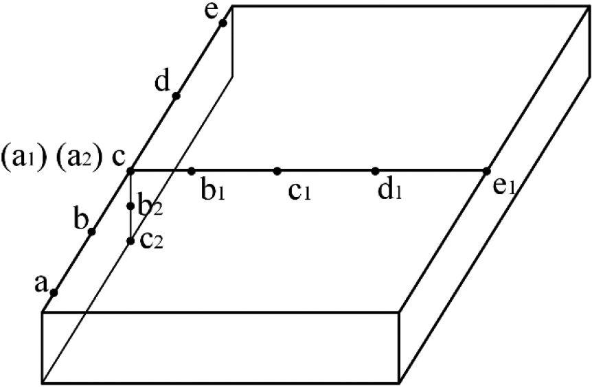

Four different cutting speeds were selected for flame cutting simulation analysis to study the effect of cutting speed on the temperature field, and the temperature cloud diagram of the cutting process is shown in Fig. 7, and the temperature unit is Celsius (^∘C).

Figure 7.

Temperature cloud chart at the 11th s at different cutting speeds.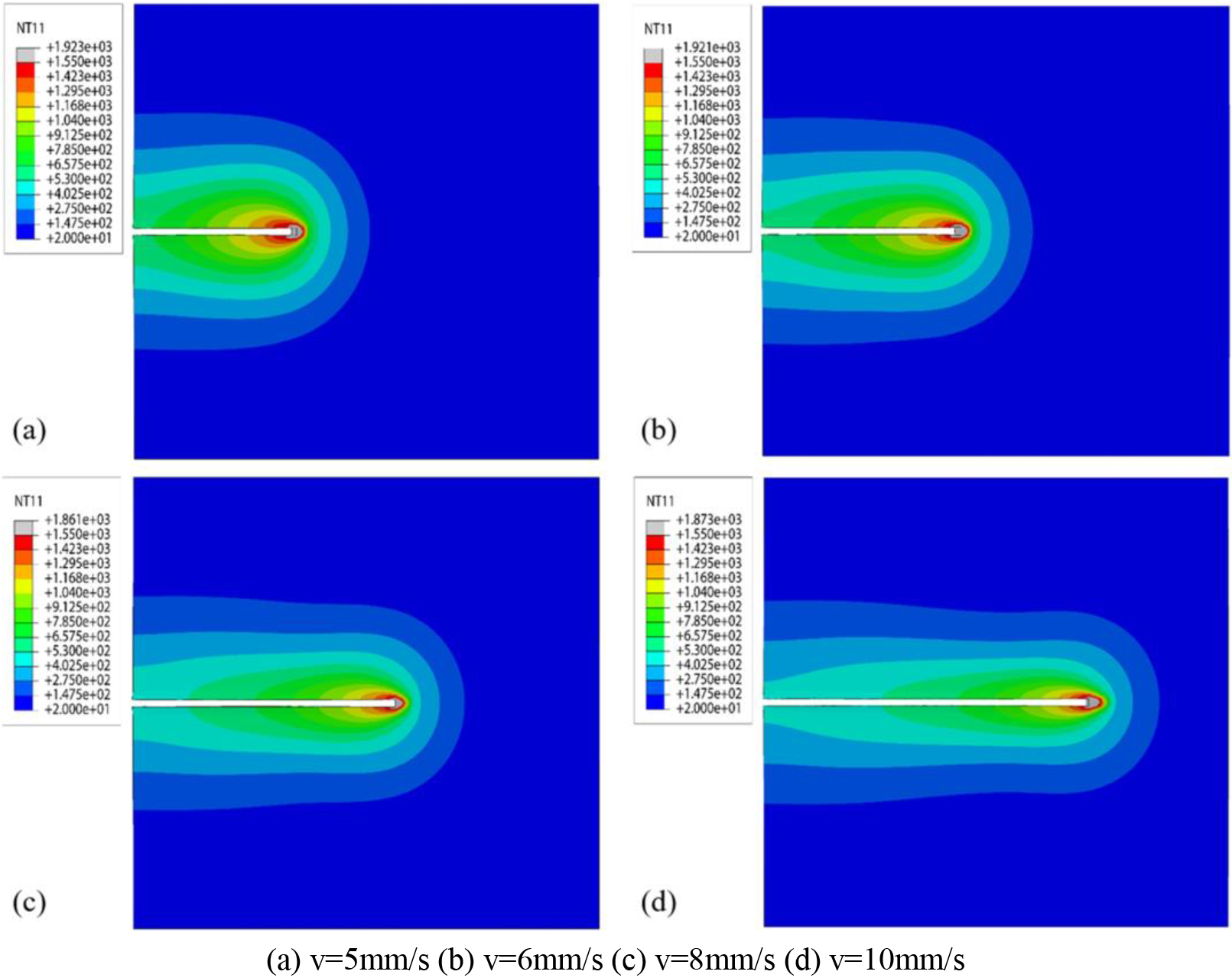

4.1.1 Analysis of temperature field at points a-e along the slotting direction

After the cutting is completed, sort out the results of the temperature data points a-e along the kerf direction, and draw the thermal cycle curve as shown in Fig. 8. Analysis of the thermal cycle diagram shows that the trend of temperature change under different cutting speeds is the same. The difference is the time it takes for each temperature data point to reach the maximum temperature and cool down to a certain temperature. The faster cutting speed makes each temperature data point reach the maximum temperature faster, and the time it takes to cool down to a certain temperature is also shorter. Analysis of the thermal cycle diagram shows that the maximum temperature of each data point is different at the same cutting speed, which is an important reason for the uneven kerf texture after cutting.

Figure 8.

Thermal cycle curves of different cutting speeds a-e temperature data points.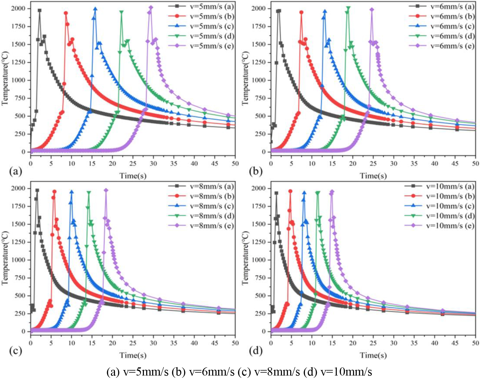

4.1.2 Analysis of temperature field at point a1-e1 perpendicular to kerf direction

After the cutting is completed, sort out the results of the temperature data points a1-e1 perpendicular to the kerf direction, and draw the thermal cycle curve as shown in Fig. 9. Analysis of the thermal cycle diagram shows that the temperature change trend of each point at different cutting speeds is the same, and the closer the point is to the kerf, the higher the temperature is. The faster cutting speed makes the temperature rise lower at the point away from the kerf, and the temperature drops faster after reaching the maximum temperature, the temperature rise of the point farthest from the kerf is very small, and the temperature of the point farthest from the kerf increases slightly, and the temperature data points have essentially the same temperature rise.

Figure 9.

Thermal cycle curves of temperature data points at different cutting speeds a1-e1.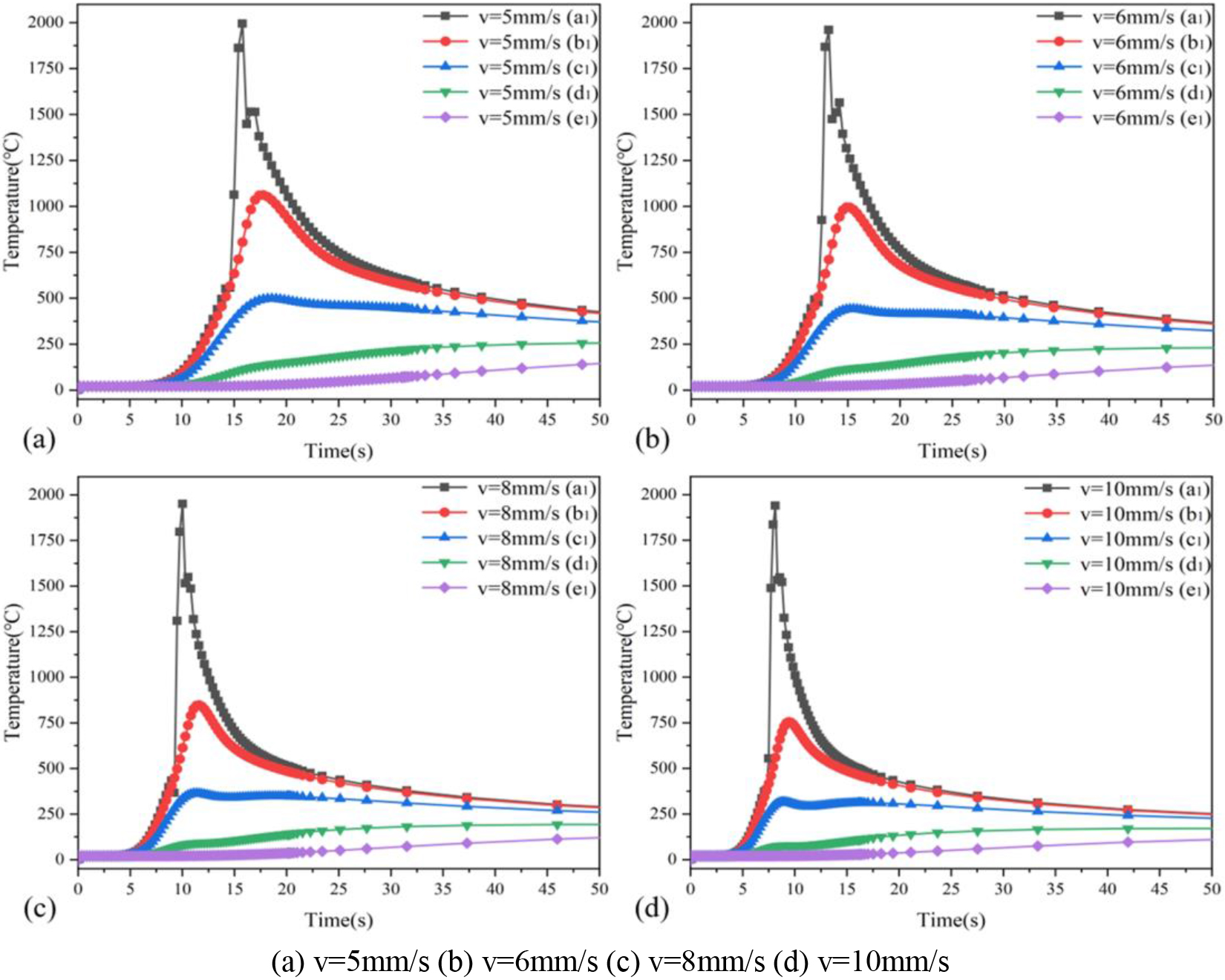

4.1.3 Analysis of temperature field at point a2-c2 along the kerf depth direction

After the cutting is completed, sort out the results of the temperature data points a2-c2 in the middle of the model along the depth direction of the kerf, and draw the thermal cycle curve as shown in Fig. 10. Analysis of the thermal cycle diagram shows that the maximum temperature that can be reached by each temperature data point on the surface of the model at different cutting speeds is higher than that of the internal temperature data point. This is due to the effect of preheating flames on the upper surface, the role of the preheating flame cannot be ignored in the simulation. As the cutting speed becomes faster, the maximum temperature that can be achieved by each temperature data point is also generally reduced. The thermal cycle of each temperature data point has a common trend. After the temperature reaches the maximum value, it first drops rapidly to a certain temperature, and then slowly cools down to a certain temperature. The faster cutting speed makes the temperature drop rate faster after each temperature data point reaches the maximum temperature, and the final temperature of each temperature data point is lower within the same cooling time.

Figure 10.

Thermal cycle curves of different cutting speeds a2-c2 temperature data points.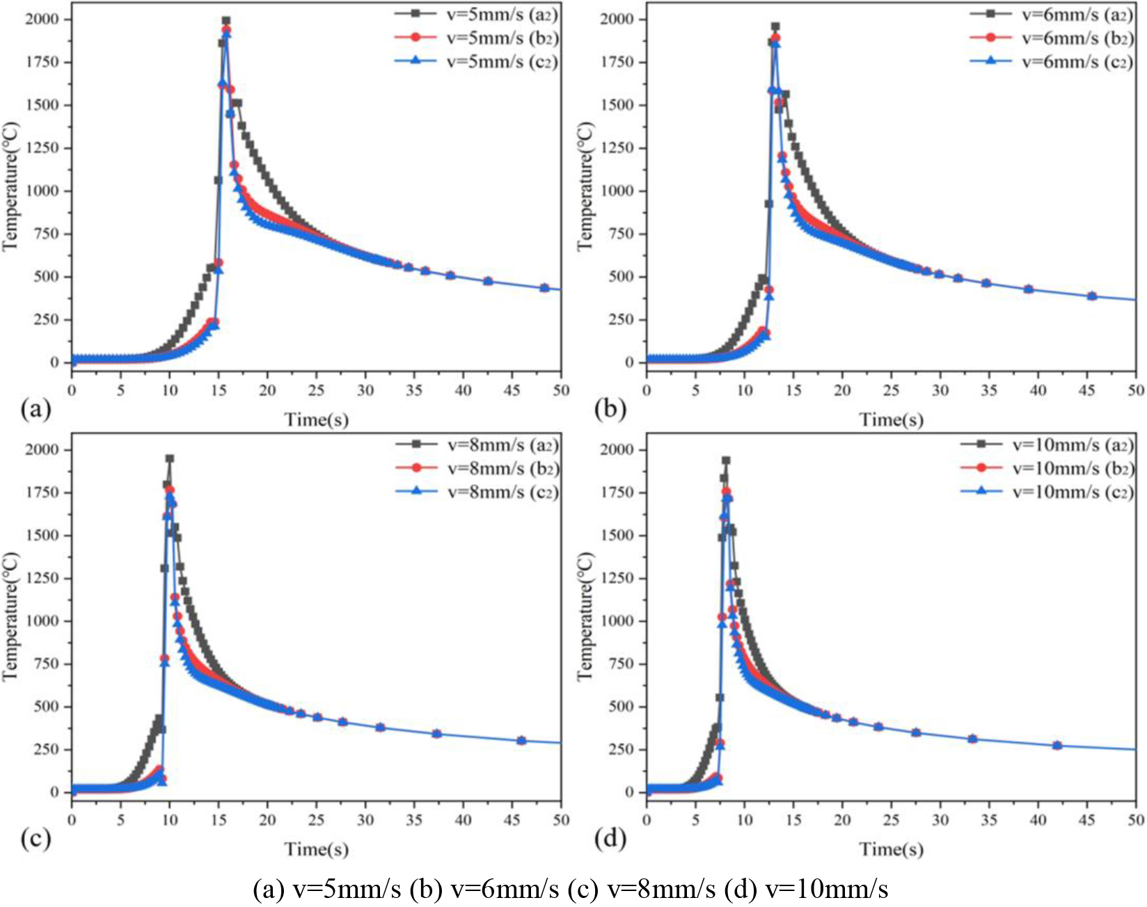

4.2 Analysis of cutting residual stress simulation results

The thermal-mechanical direct coupling method is used for flame cutting simulation, and the data of flame cutting residual stress field can be obtained at the same time as the data of cutting temperature field. According to the Von Mises yield criterion, the equivalent stress state is displayed, and the residual stress cloud diagram after cooling at different cutting speeds is obtained through numerical simulation. As shown in Fig. 11.

Figure 11.

Residual stress cloud diagram of different cutting speeds.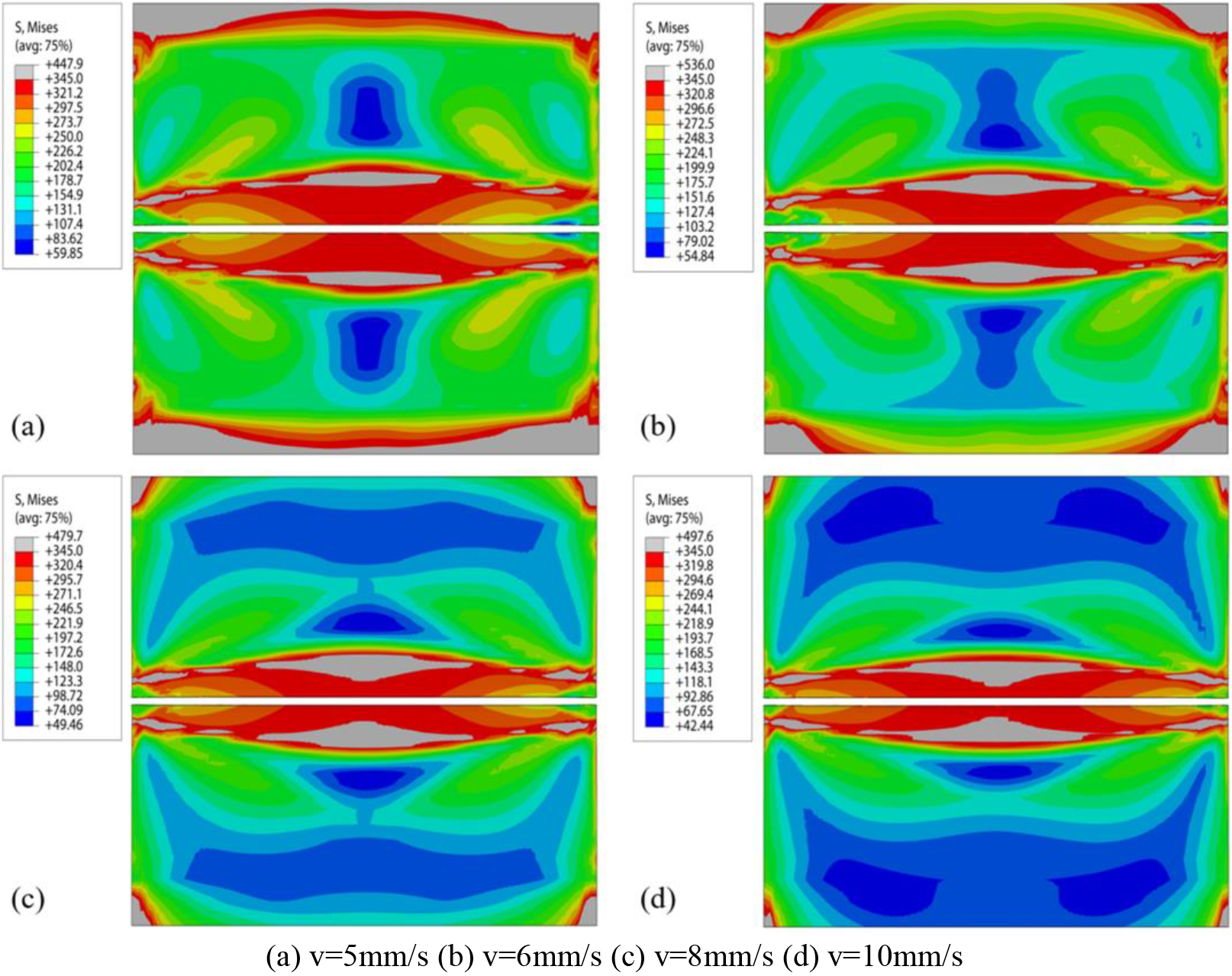

From the Mises stress cloud diagram, it can be seen that the distribution of residual stress after cutting and cooling at different cutting speeds is roughly the same. The stress in the area close to the slot is relatively large, the stress in the area away from the slot is relatively small, and the stress at the edge of the model is also large due to the constraints. Moreover, the faster cutting speed makes the stress values in most areas decrease continuously. Next, the longitudinal and transverse residual stresses on the surface of the model under different cutting speeds are analyzed, which can describe the residual stress distribution of the model more accurately.

As shown in Fig. 12, it is the cloud diagram of the distribution of longitudinal residual stress S11. It can be seen from the figure that the stress value in some areas of the cutting model exceeds the yield limit value of the model material, and the longitudinal residual stress S11 is near the kerf and the boundary area of the model. Tensile stress is present, and compressive stress is present in the area away from the kerf. The increase of cutting speed will make the area value of tensile stress area decrease continuously, while the area value of compressive stress area increases continuously. Figure 13 shows the S11 stress values extracted along the kerf direction and perpendicular to the kerf direction.

Figure 12.

Cloud diagram of longitudinal residual stress S11 at different cutting speeds.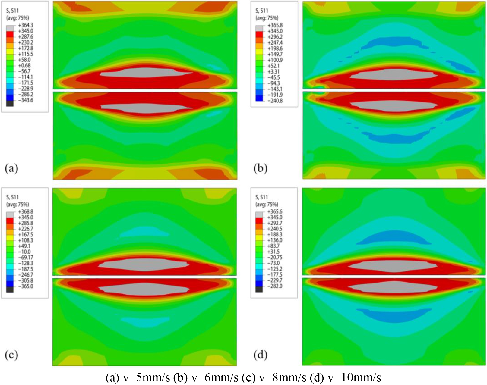

Figure 13.

S11 stress curves in different directions.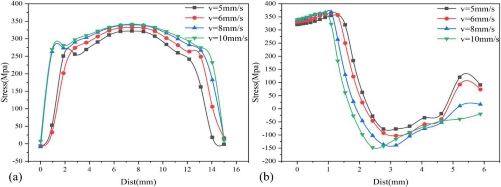

Analysis of the S11 stress curve shows that along the kerf direction, the S11 stress value is close to 0 at the cutting start point and end point, the closer to the middle of the model, the greater the value of S11, and the largest in the middle position. The faster the cutting speed, the smaller the S11 stress value corresponding to each point. Perpendicular to the kerf direction, the longitudinal residual stress S11 first presents a large tensile stress, which even exceeds the yield limit of the material, and the faster cutting speed reduces the area of the tensile stress region. After reaching the peak value of the tensile stress, the S11 stress value rapidly decrease, from tensile stress to compressive stress, and the faster cutting speed makes the peak value of compressive stress larger, and then the S11 stress value continues to increase until the boundary of the model.

As shown in Fig. 14, it is the stress cloud diagram of the transverse residual stress S22. Analyzing the S22 cloud diagram, it can be seen from the figure that the transverse residual stress S22 presents a relatively large tensile stress in the boundary area at the beginning and end of the cutting model, while it is perpendicular to the kerf model the boundary area presents a large compressive stress, and the faster cutting speed makes the values of the tensile and compressive stress areas decrease. Figure 15 shows the S22 stress values extracted along the kerf direction and perpendicular to the kerf direction.

Figure 14.

Cloud diagram of transverse residual stress S22 at different cutting speeds.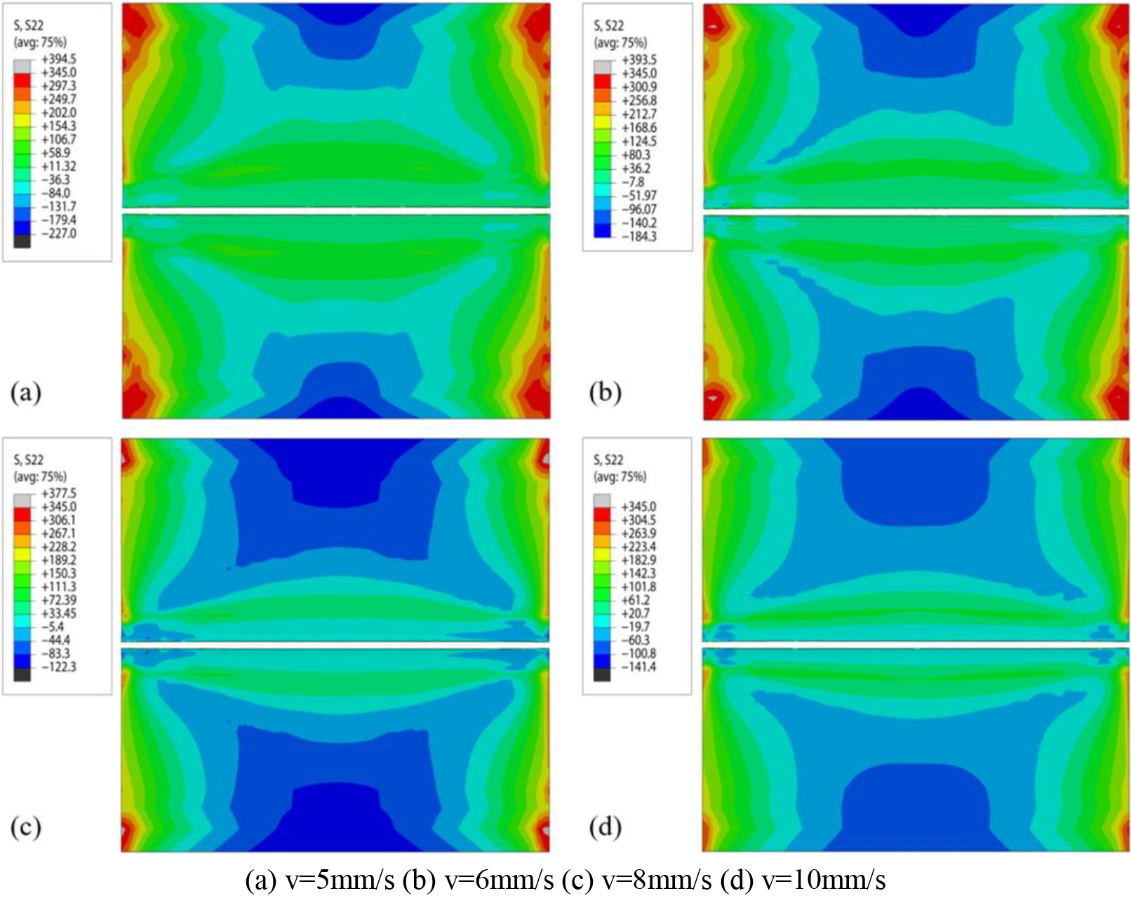

Figure 15.

S22 stress curves in different directions.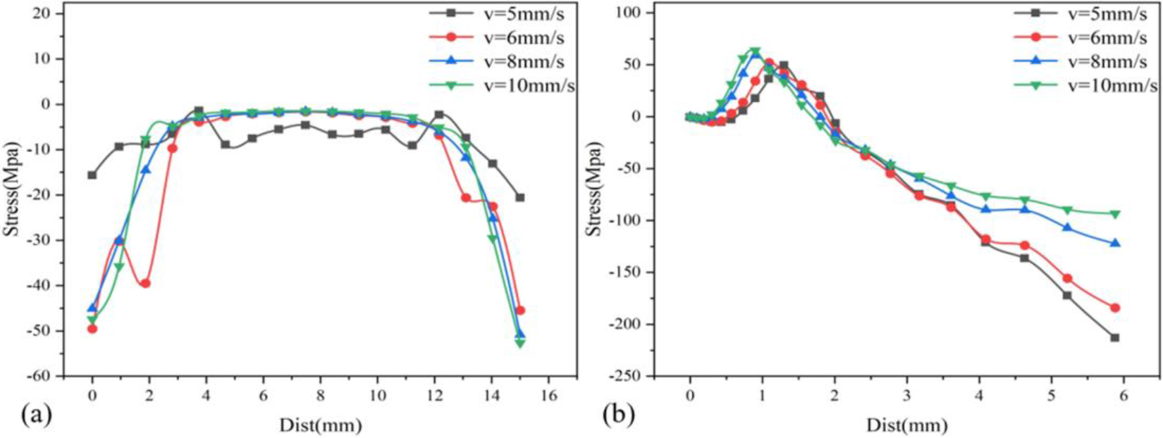

Analysis of the S22 stress curve shows that along the kerf direction, the transverse residual stress S22 presents a small compressive stress at the cutting start point and end point, and the value of S22 in the middle position of the cutting model presents a compressive stress close to 0, and different cutting speeds have a significant impact on the S22 stress value in the kerf direction has little effect. Perpendicular to the kerf direction, the transverse residual stress S22 actually presents a small tensile stress, and the faster cutting speed makes the tensile stress area smaller and the stress value larger. After reaching the peak value of the tensile stress, the S22 stress value keeps decreasing, from tensile stress becomes compressive stress, and the faster the cutting speed, the greater the compressive stress.

5. Conclusion

In this paper, ABAQUS software is used to model and simulate the flame cutting Q345D flat plate, and a new type of flame cutting composite heat source model is established. The influence of cutting speed on the cutting temperature field and residual stress distribution is studied by using the direct thermal-mechanical coupling method, and the following conclusions are obtained:

(1)

The temperature change law of each temperature measuring point is similar at different cutting speeds. Along the kerf direction, the maximum temperature difference of each temperature data point is very small, and the faster cutting speed makes the temperature decrease faster after reaching the maximum temperature; Perpendicular to the direction of the kerf, the faster cutting speed makes the temperature rise of the temperature data point away from the kerf lower, and the temperature drops faster after reaching the maximum temperature; Along the direction of the kerf depth, due to the effect of the preheating flame on the surface of the model, the maximum temperature of the internal temperature data point of the model is lower than that of the model surface data point.

(2)

For the longitudinal residual stress S11, along the kerf direction, S11 stress value at both ends of the model is close to 0,the closer to the middle of the model, the greater the S11 stress value, and the S11 stress value corresponding to each point becomes larger as the cutting speed becomes faster; perpendicular to the kerf direction, the S11 stress value first presents a large tensile stress, and the faster cutting speed makes the tensile stress area smaller. After reaching the peak value of the tensile stress, the S11 stress value gradually changes to compressive stress, and the faster cutting speed makes the peak value of compressive stress larger.

(3)

For the transverse residual stress S22, along the kerf direction, the stress value of S22 presents a small compressive stress, and different cutting speeds have basically no effect on the S22 stress value along the kerf direction; Perpendicular to the kerf direction, the S22 stress value first presents a small tensile stress, and the faster cutting speed makes the tensile stress area smaller and smaller, while the tensile stress value continues to increase, and gradually changes to compressive stress after reaching the peak value, and the faster the cutting speed, the greater the compressive stress value.

References

Kim

Chen

Majumdar

. Finite element modelling of the laser cutting process. Computers & Structures. 1993; 49(2): 231-241.

Arif

AFM

Yilbas

Aleem

. Laser cutting of thick sheet metals: Residual stress analysis. Optics & Laser Technology. 2009; 41(3): 224-232.

Yilbas

Arif

AFM

. Laser cutting of steel and thermal stress development. Optics & Laser Technology. 2011; 43(4): 830-837.

Jiao

Wang

. A numerical simulation of machining glass by dual CO2-laser beams. Optics & Laser Technology. 2008; 40(2): 297-301.

Kheloufi

Amara

Benzaoui

. Numerical Simulation of Transient Three-Dimensional Temperature and Kerf Formation in Laser Fusion Cutting. Journal of Heat Transfer. 2014; 137(11).

Zhou

Liu

Tan

. Efficient simulation of oxygen cutting using a composite heat source model. International Journal of Heat and Mass Transfer. 2013; 57(1): 304-311.

Bae

Yang

, et al., Numerical analysis of heat flow in oxy-ethylene flame cutting of steel plate. Proceedings of the Institution of Mechanical Engineers, Part B. Journal of Engineering Manufacture. 2018; 232(4): 742-751.

Thiébaud

Drezet

Lebet

. Experimental and numerical characterisation of heat flow during flame cutting of thick steel plates. Journal of Materials Processing Technology. 2014; 214(2), 304-310.

Huang

Zhang

. Distribution of cutting and welding thermal residual stress in steel bone with and without holes in the partially encased composite wall. Buildings. 2022; 12(11).

10.

Jokiaho

Laitinen

Santa-Aho

, et al., Characterization of Flame Cut Heavy Steel: Modeling of Temperature History and Residual Stress Formation. Metallurgical Materials Transactions B. 2017; 48(6): 2891-2901.

11.

Arenas

Hömberg

Lasarzik

, et al., Modelling and simulation of flame cutting for steel plates with solid phases and melting. Journal of Mathematics in Industry. 2020; 10: 1-16.

12.

Lindgren

Carlestam

Jonsson

. Computational model of flame-cutting. Eng Master Technol. 1993; 115(4): 440-445.

13.

Moradi

Moghadam

Shamsborhan

, et al. Simulation, statistical modeling, and optimization of CO2 laser cutting process of polycarbonate sheets. Optik. 2021; 225: 164932.

14.

Peirovi

Pourasghar

Nejad

, et al. A study on the different finite element approaches for laser cutting of aluminum alloy sheet. The International Journal of Advanced Manufacturing Technology. 2017; 93(1): 1399-1413.

15.

Sharifi

Akbari

. Experimental investigation of the effect of process parameters on cutting region temperature and cutting edge quality in laser cutting of AL6061T6 alloy. Optik. 2019; 184: 457-463.

16.

Xiong