Multi-fidelity Kriging extrapolation together with CFD for the design of the cross-section of a falling lifeboat

Abstract

Surrogate modelling techniques such as Kriging are a popular means for cheaply emulating the response of expensive Computational Fluid Dynamics (CFD) simulations. These surrogate models are often used for exploring a parameterised design space and identifying optimal designs. Multi-fidelity Kriging extends the methodology to incorporate data of variable accuracy and costs to create a more effective surrogate. This work recognises that the grid convergence property of CFD solvers is currently an unused source of information and presents a novel method that, by leveraging the data structure implied by grid convergence, could further improve the performance of the surrogate model and the corresponding optimisation process. Grid convergence states that the simulation solution converges to the true simulation solution as the numerical grid is refined. The proposed method is tested with realistic multi-fidelity data acquired with CFD simulations. The performance of the surrogate model is comparable to an existing method, and likely more robust. More research is needed to explore the full potential of the proposed method. Code has been made available online at https://github.com/robertwenink/MFK-Extrapolation.

1. Introduction

1.1. Motivation

Automatic design procedures based on Computational Fluid Dynamics (CFD) simulations are becoming increasingly important in practical ship design [36]. For an efficient optimisation phase of such a design procedure, accurate high-dimensional surrogate modelling is essential [43]. A surrogate model provides a cheap substitute for an expensive (CFD) simulation, enabling us to feasibly approximate and explore the design space. To illustrate the effectiveness and promise of using surrogate models in naval optimisation routines, Scholcz and Veldhuis [37] show that Surrogate-Based Global optimisation (SBGO) of a tanker’s hull reduces the required computational time from two weeks to only a day when compared with a direct optimisation algorithm. This is important since Raven and Scholcz [34] state that the time available for hull shape optimisation with the goal of, for instance, wave resistance minimisation is usually only one to two weeks or even less.

However, SBGO suffers from the curse of dimensionality [27]. Here, the curse of dimensionality refers to the exponential growth of the design-space volume when the number of dimensions or design variables increases, thereby drastically increasing the number of (expensive) simulations required to cover this volume and reliably construct the surrogate model. In other words, if we increase the number of design variables we optimise over, we drastically need to increase the number of CFD simulations, which is costly or even infeasible. Simultaneously, high-dimensional design spaces naturally arise in naval ship design [37], making this curse of dimensionality a limiting problem for using SBGO in practice.

Multi-fidelity modelling can improve the efficiency of SBGO, by using the usual expensive and precise data together with less expensive but less accurate data. Results as early as that of Leifsson et al. [22] show that optimised hull designs can be obtained at over 94% lower computational cost when using multi-fidelity optimisation as compared to a direct high-fidelity optimisation algorithm. However, these results typically do not scale to more design variables.

We want to lessen the effects of the curse of dimensionality even further and enable ourselves to feasibly solve more complex problems of higher dimensionality, or to solve problems less costly and more accurately in general. Shan and Wang [38] survey strategies of solving high-dimensional expensive black-box problems. These strategies include problem decomposition, screening (e.g. Global Sensitivity Analysis), mapping (e.g. lossless projection of high-dimensional spaces onto lower-dimensional spaces; or multi-fidelity approaches that map a lower-fidelity onto a higher-fidelity model (such as considered in this work), and (adaptive) space reduction. From these, Shan and Wang [38] mark mapping as a promising approach and note that research does not take advantage of the characteristics of the underlying expensive functions. Wu and Wang [46] reiterate this conclusion, demonstrating that this research direction still holds relevance today.

In this work, we recognise that the grid convergence property of CFD solvers is currently an unused source of information that could further improve the performance of the surrogate model and the corresponding optimisation process. Grid convergence states that the simulation solution converges to the ‘true’ simulation solution as the grid is refined. CFD simulations reported by for instance Eijk and Wellens [40] show the clear presence of grid convergence. Therefore, this work explores a novel hierarchical multi-fidelity mapping method exploiting this grid convergence information to relieve the effects of the curse of dimensionality at the expensive high fidelity.

1.2. Method background

Kriging, also known as a form of Gaussian Process Regression [32], is a particularly popular surrogate modelling technique due to two reasons. First, Kriging provides the best linear unbiased prediction (BLUP) when the assumption of Gaussian correlations between data samples holds [35]. Second, Kriging provides an estimation of the mean squared error corresponding to that prediction [9].

Kriging receives its name from Krige [19,20], who used a precursor method to estimate gold concentrations based on only a few boreholes. It was further mathematically developed by Matheron [25] and has been popularised for use outside the field of geostatistics by Sacks [35]. Jones [14] and Forrester et al. [9] provide a gentle and intuitive introduction to (Ordinary) Kriging.

Kriging and other forms of Gaussian Process Regression are the most popular surrogate models for use in Bayesian optimisation [27], of which the Efficient Global Optimisation (EGO) algorithm [13] is one form. The EGO algorithm adaptively samples additional points based on the Expected Improvement criterion [13], which is formulated using the estimated mean squared error that Kriging provides. Using this criterion, EGO provably converges to the global optimum in an optimisation process [24], although it may exhaustively sample around local optima [8].

In contrast to Gaussian Process Regression, Kriging in principle is an interpolating formulation, which causes problems in the presence of noisy data. To solve this, Forrester et al. [7] show how to introduce regression terms to the Kriging formulation in coherence with the EGO method through a process called re-interpolation. Jones [14] discusses the relation of Kriging with respect to other surrogate modelling methods and explores possible improvements to EGO and the Expected Improvement criterion. As one of the most promising directions for further work, he hinted towards multi-fidelity simulation: using expensive high-precision simulations together with simulations of a lower precision but a much lower cost. This enables us to respectively balance exploitation and exploration of the search space and thereby cut costs while improving the quality of the surrogate.

Since then, Multi-Fidelity Kriging has received significant research effort, see for instance the review papers of Fernández-Godino et al. [10], Peherstorfer et al. [28], Viana et al. [43]. Kennedy and O’Hagan [15] mathematically formulated the fundamentals, while Forrester et al. [8] provides a more transparent overview. Gratiet and Garnier [21] show that the model of Kennedy and O’Hagan [15] can be equivalently but more cheaply formulated as recursively nested independent Kriging problems, one for each fidelity level. Perdikaris et al. [30] improve upon this work by generalising the linear autoregressive1

¹

Meaning that the relations between fidelity levels and the regression parameters are directly solved in the linear system.

formulation of Gratiet and Garnier [21] to better accommodate non-linear-relations.

Korondi et al. [17], Meliani et al. [26] use the recursive formulation of Gratiet and Garnier [21] to introduce a multi-fidelity approach to the EGO algorithm and formulate level-selection criteria that balance the expected reduction of the prediction variance with the costs of sampling a given level. The combination of Gratiet and Garnier [21] together with the multi-fidelity SBGO method of Meliani et al. [26] will serve as a reference to the method proposed in this work since that combination will feature the so-called nested Design of Experiments (DoE), a sampling strategy that provides the most complete information on the relation between the fidelities [15].

Optimisation methods based on Multi-Fidelity Kriging hold promise in maritime engineering considering the following accounts. Raven [33], Raven and Scholcz [12] apply Multi-Fidelity Kriging in a ship hull form optimisation with a dense set of potential flow results and a coarse set of RANS data, and positively compared the result with the single-fidelity formulation. Korondi et al. [18] performs reliability-based optimisation of a ducted propeller using an EGO-like strategy and a multi-fidelity Kriging surrogate. Although performed under compressible flow conditions, the same techniques are interesting to incompressible flows. Liu et al. [23] uses viscous and potential flow calculations as the high- and low-fidelity respectively and shows the multi-fidelity Kriging approach can obtain a more optimal hydrodynamic hull form than the single-fidelity model alone.

Other than in these accounts, to the authors’ knowledge, Multi-Fidelity Kriging does not seem to have been applied within maritime engineering, presumably because the increased complexity of the computational setup versus the perceived potential benefit. There are still unresolved questions regarding when it is advantageous to use a multi-fidelity over the standard single-fidelity approach [11,17,39] in terms of accuracy, cost, and assumed data characteristics.

1.3. Objective

The main research objective that is investigated is how to leverage the grid convergence property of CFD solvers in order to reduce the number of expensive high-fidelity samples required for an accurate (multi-fidelity) Kriging surrogate. Using this property can accelerate surrogate-based global design optimisation in maritime engineering. CFD with a free surface description is used to computed the accelerations for stylized bow shapes of a falling life boat. The main assumption in reaching the objective is that value differences of the objective function that minimized the accelerations, implied by the grid convergence property of a CFD solver, are proportional from one point in the design space to another. To our knowledge the assumption has not been investigated in the context of Kriging or Gaussian Processes for the purpose of Bayesian Optimisation.

2. Methodology

When we take a look at the results of Forrester et al. [8] in Fig. 1, and later those of Meliani et al. [26] in a fully MF-EGO setting, we notice that although we are only interested in the optimum solution we still need to construct the multi-fidelity surrogate model by sampling the high-fidelity across the full domain. Effectively we need to sample the expensive high-fidelity truth in areas that ultimately are not of interest to an optimisation problem, and therefore will not be directly used. This seems to be a waste of our resources, especially since the high-fidelity per definition is often much more expensive than the low-fidelity while both are generally required to be highly correlated [39].

Fig. 1.

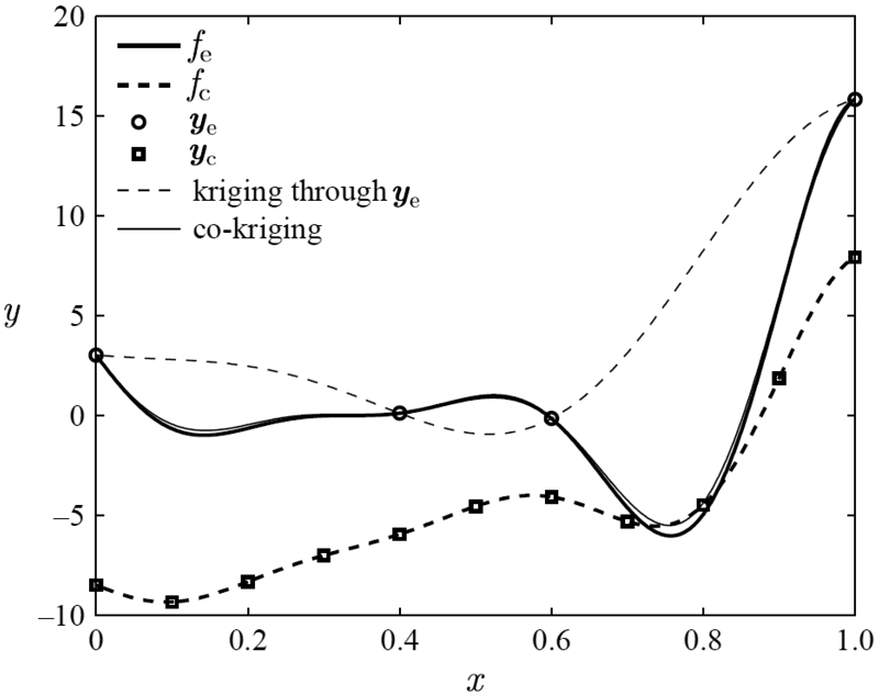
Image from Forrester et al. [8] to showcase multi-fidelity Kriging. Here ${\mathit{y}}_{\mathit{c}}$ represent low-fidelity samples, ${\mathit{y}}_{\mathit{e}}$ represent high-fidelity samples, and ‘co-Kriging’ is the surrogate that uses the samples at both fidelity levels to find an optimum.

Due to the high required correlation between fidelity levels, we implicitly assume to be able to identify regions of interest based on the low fidelity and only sample the high fidelity there. However, this approach presents a problem already observed in the toy case of Forrester et al. [8], where the low-fidelity optimum is only a local optimum of the ‘truth’. Compared to the reference method with two fidelity levels [21,26], our proposed method will feature three fidelity levels, low, medium and high, and will formulate a surrogate model from the combination of samples at these fidelity levels and the assumption of uniform grid convergence, thereby arriving at the formulation of the main assumption as stated together with the objective.

In the following, we exploit this assumption and project the information of as few as a single high-fidelity sample onto the full input domain. We thereby retrieve an approximate Kriging model of the high-fidelity (near) truth, which at the very least should be indicative of areas of interest to an optimisation routine. Then, the adaptive sampling of the EGO algorithm can be performed as usual but at a lower cost of the initial surrogate model in terms of sampling the high-fidelity.

2.1. Basic formulation

We want to predict an unknown higher fidelity level based on as few samples as possible at that unknown level. To do this, we will estimate the training points of the Kriging model at an unknown level $\mathit{l}+1$ , initially based upon only one actual high-fidelity sample at a location of interest to our optimisation. We retrieve an initial sample ${\mathit{z}}_{\mathit{l}+1\mathrm{,}{\mathit{x}}_0}$ with ${\mathit{x}}_0={\mathit{X}}_{\mathit{l}}[argmin\mathrm{(}{\mathit{Z}}_{\mathit{l}}\mathrm{)}]$ and intuitively determine the multiplicative difference: $$\begin{array}{c}{\mathit{d}}_{{\mathit{x}}_0}={\displaystyle \frac{{\mathit{z}}_{\mathit{l}+1\mathrm{,}{\mathit{x}}_0}}{{\mathit{z}}_{\mathit{l}\mathrm{,}{\mathit{x}}_0}}}.\end{array}$$ Here, l denotes the currently known level, and $\mathit{l}+1$ is the level we want to predict. We would then use this discrepancy to predict the value at some other location ${\mathit{x}}_{\ast }$ of level $\mathit{l}+1$ as: $$\begin{array}{c}{\mathit{z}}_{\mathit{p}\mathrm{,}{\mathit{x}}_{\ast }}={\mathit{z}}_{\mathit{l}\mathrm{,}{\mathit{x}}_{\ast }}·{\mathit{d}}_{{\mathit{x}}_0}.\end{array}$$ We use subscript p to more clearly indicate a predicted value at level $\mathit{l}+1$ . Now, we would like the discrepancy ${\mathit{d}}_{{\mathit{x}}_0}$ to scale according to the increase we observe between the two lower fidelity levels at this other point ${\mathit{x}}_{\ast }$ to obtain discrepancy ${\mathit{d}}_{{\mathit{x}}_{\ast }}$ . That is, we match the ratios of the differences between levels ( $\mathit{l}-1$ , l) and (l, $\mathit{l}+1$ ) at locations ${\mathit{x}}_0$ and ${\mathit{x}}_{\ast }$ , thereby retrieving: $$\begin{array}{rl}{\displaystyle \frac{{\mathit{z}}_{\mathit{l}\mathrm{,}{\mathit{x}}_{\ast }}-{\mathit{z}}_{\mathit{l}-1\mathrm{,}{\mathit{x}}_{\ast }}}{{\mathit{z}}_{\mathit{l}\mathrm{,}{\mathit{x}}_0}-{\mathit{z}}_{\mathit{l}-1\mathrm{,}{\mathit{x}}_0}}}& ={\displaystyle \frac{{\mathit{z}}_{\mathit{l}+1\mathrm{,}{\mathit{x}}_{\ast }}-{\mathit{z}}_{\mathit{l}\mathrm{,}{\mathit{x}}_{\ast }}}{{\mathit{z}}_{\mathit{l}+1\mathrm{,}{\mathit{x}}_0}-{\mathit{z}}_{\mathit{l}\mathrm{,}{\mathit{x}}_0}}}\\ & ={\displaystyle \frac{{\mathit{z}}_{\mathit{l}\mathrm{,}{\mathit{x}}_{\ast }}·{\mathit{d}}_{{\mathit{x}}_{\ast }}-{\mathit{z}}_{\mathit{l}\mathrm{,}{\mathit{x}}_{\ast }}}{{\mathit{z}}_{\mathit{l}\mathrm{,}{\mathit{x}}_0}·{\mathit{d}}_{{\mathit{x}}_0}-{\mathit{z}}_{\mathit{l}\mathrm{,}{\mathit{x}}_0}}}.\end{array}$$ Rewriting in order to get an expression for ${\mathit{d}}_{{\mathit{x}}_{\ast }}$ : $$\begin{array}{c}{\mathit{d}}_{{\mathit{x}}_{\ast }}={\displaystyle \frac{{\mathit{z}}_{\mathit{l}\mathrm{,}{\mathit{x}}_0}{\mathit{z}}_{\mathit{l}\mathrm{,}{\mathit{x}}_{\ast }}-{\mathit{z}}_{\mathit{l}-1\mathrm{,}{\mathit{x}}_{\ast }}{\mathit{z}}_{\mathit{l}\mathrm{,}{\mathit{x}}_0}}{{\mathit{z}}_{\mathit{l}\mathrm{,}{\mathit{x}}_0}{\mathit{z}}_{\mathit{l}\mathrm{,}{\mathit{x}}_{\ast }}-{\mathit{z}}_{\mathit{l}-1\mathrm{,}{\mathit{x}}_0}{\mathit{z}}_{\mathit{l}\mathrm{,}{\mathit{x}}_{\ast }}}}·\mathrm{(}{\mathit{d}}_{{\mathit{x}}_0}-1\mathrm{)}+1\end{array}$$ Equivalently, rewriting this to a physically much more logical form in which we predict a high-fidelity point directly: $$\begin{array}{}\text{(1)}& {\mathit{z}}_{\mathit{p}\mathrm{,}{\mathit{x}}_{\ast }}={\displaystyle \frac{{\mathit{z}}_{\mathit{l}+1\mathrm{,}{\mathit{x}}_0}-{\mathit{z}}_{\mathit{l}\mathrm{,}{\mathit{x}}_0}}{{\mathit{z}}_{\mathit{l}\mathrm{,}{\mathit{x}}_0}-{\mathit{z}}_{\mathit{l}-1\mathrm{,}{\mathit{x}}_0}}}·\mathrm{(}{\mathit{z}}_{\mathit{l}\mathrm{,}{\mathit{x}}_{\ast }}-{\mathit{z}}_{\mathit{l}-1\mathrm{,}{\mathit{x}}_{\ast }}\mathrm{)}+{\mathit{z}}_{\mathit{l}\mathrm{,}{\mathit{x}}_{\ast }}\end{array}$$

2.2. Incorporating noise and variance

Noise and variance are in principle present in each of the values used in Eq. (1).

Note again that sampling noise of numerical origin can be regressed and estimated by introducing an additional hyperparameter. We can then describe the noise using a Gaussian variance that is fully integrated with the Kriging model prediction variance.

To project this combination of noise and Kriging variance onto our estimation of the high-fidelity, we should thus incorporate them into Eq. (1). Noticing each z in Eq. (1) is actually the mean of a Gaussian, we can alternatively write the corresponding Gaussian as: $$\begin{array}{}\text{(2)}& \mathcal{N}\mathrm{(}{\mathit{z}}_{\mathit{l}\mathrm{,}\mathit{x}}\mathrm{,}{\mathit{\sigma }}_{\mathit{l}\mathrm{,}\mathit{x}}\mathrm{)}={\mathit{z}}_{\mathit{l}\mathrm{,}\mathit{x}}+\mathcal{N}\mathrm{(}0\mathrm{,}1\mathrm{)}·{\mathit{\sigma }}_{\mathit{l}\mathrm{,}\mathit{x}}={\mathit{z}}_{\mathit{l}\mathrm{,}\mathit{x}}+{\mathcal{N}}_{\mathit{l}\mathrm{,}\mathit{x}}·{\mathit{\sigma }}_{\mathit{l}\mathrm{,}\mathit{x}}.\end{array}$$ Here, ${\mathcal{N}}_{\mathit{l}\mathrm{,}\mathit{x}}$ is used as a shorthand notation for the standard normal distribution $\mathcal{N}\mathrm{(}0\mathrm{,}1\mathrm{)}$ , corresponding to level l and location x. We now make three assumptions:

The high-fidelity sample ${\mathit{z}}_{\mathit{l}+1\mathrm{,}{\mathit{x}}_0}$ exhibits no noise or variance.

In other words, we assume the sampled (near) truth to be sufficiently precise such that it exhibits relatively little to no noise. In reality however, this is a practical consideration since we will have an insufficient amount of high-fidelity samples to pre-emptively obtain an accurate noise estimate.

At location ${\mathit{x}}_0$ , the Kriging variances of levels l and $\mathit{l}-1$ are i.i.d. Gaussians.

As we will see at the end of this section, it only makes sense to sample all three involved levels at location ${\mathit{x}}_0$ , leading to a nested DoE. This implies that at ${\mathit{x}}_0$ there will be no (cross-correlated) Kriging predictions and variances present, but only noise estimates. These noise estimates are per definition i.i.d., see for instance [7,21].

At location ${\mathit{x}}_{\ast }$ , ${\mathcal{N}}_{\mathit{l}\mathrm{,}{\mathit{x}}_{\ast }}$ and ${\mathcal{N}}_{\mathit{l}-1\mathrm{,}{\mathit{x}}_{\ast }}$ are perfectly negatively correlated. In effect, the difference $\mathcal{N}\mathrm{(}{\mathit{z}}_{\mathit{l}\mathrm{,}{\mathit{x}}_{\ast }}\mathrm{,}{\mathit{\sigma }}_{\mathit{l}\mathrm{,}{\mathit{x}}_{\ast }}\mathrm{)}-\mathcal{N}\mathrm{(}{\mathit{z}}_{\mathit{l}-1\mathrm{,}{\mathit{x}}_{\ast }}\mathrm{,}{\mathit{\sigma }}_{\mathit{l}-1\mathrm{,}{\mathit{x}}_{\ast }}\mathrm{)}$ is described by $\mathcal{N}\mathrm{(}{\mathit{z}}_{\mathit{l}\mathrm{,}{\mathit{x}}_{\ast }}-{\mathit{z}}_{\mathit{l}-1\mathrm{,}{\mathit{x}}_{\ast }}\mathrm{,}{\mathit{\sigma }}_{\mathit{l}\mathrm{,}{\mathit{x}}_{\ast }}+{\mathit{\sigma }}_{\mathit{l}-1\mathrm{,}{\mathit{x}}_{\ast }}\mathrm{)}$

Although the actual distribution of the expected difference between $\mathcal{N}\mathrm{(}{\mathit{z}}_{\mathit{l}\mathrm{,}{\mathit{x}}_{\ast }}\mathrm{,}{\mathit{\sigma }}_{\mathit{l}\mathrm{,}{\mathit{x}}_{\ast }}\mathrm{)}$ and $\mathcal{N}\mathrm{(}{\mathit{z}}_{\mathit{l}-1\mathrm{,}{\mathit{x}}_{\ast }}\mathrm{,}{\mathit{\sigma }}_{\mathit{l}-1\mathrm{,}{\mathit{x}}_{\ast }}\mathrm{)}$ is less pessimistic in terms of variance and not necessarily normally distributed, this description provides the right variance sign (variances generally amplify each other) and provides a stronger parallel with the multi-fidelity methodology of Gratiet and Garnier [21].

Using the notation of Eq. (2) and incorporating the above assumptions into Eq. (1) retrieves the formulation: $$\begin{array}{rl}{\mathit{z}}_{\mathit{p}\mathrm{,}{\mathit{x}}_{\ast }}+{\mathcal{N}}_{{\mathit{x}}_{\ast }}{\mathit{\sigma }}_{\mathit{p}\mathrm{,}{\mathit{x}}_{\ast }}& =\mathit{f}·\mathrm{(}{\mathit{z}}_{\mathit{l}\mathrm{,}{\mathit{x}}_{\ast }}-{\mathit{z}}_{\mathit{l}-1\mathrm{,}{\mathit{x}}_{\ast }}+{\mathcal{N}}_{{\mathit{x}}_{\ast }}·\mathrm{(}{\mathit{\sigma }}_{\mathit{l}\mathrm{,}{\mathit{x}}_{\ast }}+{\mathit{\sigma }}_{\mathit{l}-1\mathrm{,}{\mathit{x}}_{\ast }}\mathrm{)}\mathrm{)}+{\mathit{z}}_{\mathit{l}\mathrm{,}{\mathit{x}}_{\ast }}\\ \text{(3a)}& & +{\mathcal{N}}_{{\mathit{x}}_{\ast }}{\mathit{\sigma }}_{\mathit{l}\mathrm{,}{\mathit{x}}_{\ast }}\text{(3b)}& \text{where}\mathit{f}& ={\displaystyle \frac{{\mathit{z}}_{\mathit{l}+1\mathrm{,}{\mathit{x}}_0}-{\mathit{z}}_{\mathit{l}\mathrm{,}{\mathit{x}}_0}-{\mathcal{N}}_{\mathit{l}\mathrm{,}{\mathit{x}}_0}{\mathit{\sigma }}_{\mathit{l}\mathrm{,}{\mathit{x}}_0}}{{\mathit{z}}_{\mathit{l}\mathrm{,}{\mathit{x}}_0}-{\mathit{z}}_{\mathit{l}-1\mathrm{,}{\mathit{x}}_0}+{\mathcal{N}}_{\mathit{l}\mathrm{,}{\mathit{x}}_0}{\mathit{\sigma }}_{\mathit{l}\mathrm{,}{\mathit{x}}_0}-{\mathcal{N}}_{\mathit{l}-1\mathrm{,}{\mathit{x}}_0}{\mathit{\sigma }}_{\mathit{l}-1\mathrm{,}{\mathit{x}}_0}}}.\end{array}$$ Since the terms ${\mathit{\sigma }}_{{\mathit{x}}_{\mathit{l}\mathrm{,}0}}$ , ${\mathit{\sigma }}_{{\mathit{x}}_{\mathit{l}-1\mathrm{,}0}}$ , ${\mathit{z}}_{{\mathit{x}}_{\mathit{l}\mathrm{,}0}}$ , ${\mathit{z}}_{{\mathit{x}}_{\mathit{l}-1\mathrm{,}0}}$ in fraction f of Eq. (3a) and (3b) are known and constant, we can numerically compute the corresponding expectation ${\mathit{E}}_{\mathit{f}}$ and variance ${\mathit{S}}_{\mathit{f}}$ as a function of ${\mathcal{N}}_{{\mathit{x}}_{\mathit{l}\mathrm{,}0}}$ and ${\mathcal{N}}_{{\mathit{x}}_{\mathit{l}-1\mathrm{,}0}}$ : $$\begin{array}{}\text{(4a)}& {\mathit{E}}_{\mathit{f}}& =\mathit{E}[\mathit{f}\mathrm{(}{\mathcal{N}}_{{\mathit{x}}_{\mathit{l}\mathrm{,}0}}\mathrm{,}{\mathcal{N}}_{{\mathit{x}}_{\mathit{l}-1\mathrm{,}0}}\mathrm{)}];\text{(4b)}& {\mathit{S}}_{\mathit{f}}& =\mathit{E}\left[{\mathrm{(}\mathit{f}\mathrm{(}{\mathcal{N}}_{{\mathit{x}}_{\mathit{l}\mathrm{,}0}}\mathrm{,}{\mathcal{N}}_{{\mathit{x}}_{\mathit{l}-1\mathrm{,}0}}\mathrm{)}-{\mathit{E}}_{\mathit{f}}\mathrm{)}}^2\right].\end{array}$$ Note that the calculated variance ${\mathit{S}}_{\mathit{f}}$ is generally not a normal Gaussian, but will be treated as such in the following. Equation (3a) and (3b) can now be rewritten to: $$\begin{array}{rl}{\mathit{z}}_{\mathit{p}\mathrm{,}{\mathit{x}}_{\ast }}+{\mathcal{N}}_{{\mathit{x}}_{\ast }}{\mathit{\sigma }}_{\mathit{p}\mathrm{,}{\mathit{x}}_{\ast }}& =\mathrm{(}{\mathit{E}}_{\mathit{f}}+{\mathcal{N}}_{{\mathit{x}}_0^{\ast }}{\mathit{S}}_{\mathit{f}}\mathrm{)}·\mathrm{(}{\mathit{z}}_{\mathit{l}\mathrm{,}{\mathit{x}}_{\ast }}-{\mathit{z}}_{\mathit{l}-1\mathrm{,}{\mathit{x}}_{\ast }}+{\mathcal{N}}_{{\mathit{x}}_{\ast }}\mathrm{(}{\mathit{\sigma }}_{\mathit{l}\mathrm{,}{\mathit{x}}_{\ast }}+{\mathit{\sigma }}_{\mathit{l}-1\mathrm{,}{\mathit{x}}_{\ast }}\mathrm{)}\mathrm{)}\\ & +{\mathit{z}}_{\mathit{l}\mathrm{,}{\mathit{x}}_{\ast }}+{\mathcal{N}}_{{\mathit{x}}_{\ast }}{\mathit{\sigma }}_{\mathit{l}\mathrm{,}{\mathit{x}}_{\ast }}\\ & =\mathrm{(}{\mathit{E}}_{\mathit{f}}+{\mathcal{N}}_{{\mathit{x}}_0^{\ast }}{\mathit{S}}_{\mathit{f}}\mathrm{)}·\mathrm{(}\mathrm{\Delta }{\mathit{z}}_{{\mathit{x}}_{\ast }}+{\mathcal{N}}_{{\mathit{x}}_{\ast }}\mathrm{\Delta }{\mathit{\sigma }}_{{\mathit{x}}_{\ast }}\mathrm{)}+{\mathit{z}}_{\mathit{l}\mathrm{,}{\mathit{x}}_{\ast }}+{\mathcal{N}}_{{\mathit{x}}_{\ast }}{\mathit{\sigma }}_{\mathit{l}\mathrm{,}{\mathit{x}}_{\ast }}\\ & =\mathrm{(}{\mathit{E}}_{\mathit{f}}\mathrm{\Delta }{\mathit{z}}_{{\mathit{x}}_{\ast }}+{\mathit{z}}_{\mathit{l}\mathrm{,}{\mathit{x}}_{\ast }}\mathrm{)}+\mathrm{(}{\mathcal{N}}_{{\mathit{x}}_{\ast }}\mathrm{\Delta }{\mathit{\sigma }}_{{\mathit{x}}_{\ast }}\mathrm{(}{\mathit{E}}_{\mathit{f}}+{\mathcal{N}}_{{\mathit{x}}_0^{\ast }}{\mathit{S}}_{\mathit{f}}\mathrm{)}\\ \text{(5)}& & +\mathrm{\Delta }{\mathit{z}}_{{\mathit{x}}_{\ast }}·{\mathcal{N}}_{{\mathit{x}}_0^{\ast }}{\mathit{S}}_{\mathit{f}}+{\mathcal{N}}_{{\mathit{x}}_{\ast }}{\mathit{\sigma }}_{\mathit{l}\mathrm{,}{\mathit{x}}_{\ast }}\mathrm{)}.\end{array}$$ This defines $\mathrm{\Delta }{\mathit{z}}_{{\mathit{x}}_{\ast }}$ and $\mathrm{\Delta }{\mathit{\sigma }}_{{\mathit{x}}_{\ast }}$ as: $$\begin{array}{}\text{(6a)}& \mathrm{\Delta }{\mathit{z}}_{{\mathit{x}}_{\ast }}& ={\mathit{z}}_{\mathit{l}\mathrm{,}{\mathit{x}}_{\ast }}-{\mathit{z}}_{\mathit{l}-1\mathrm{,}{\mathit{x}}_{\ast }}\text{(6b)}& \mathrm{\Delta }{\mathit{\sigma }}_{{\mathit{x}}_{\ast }}& ={\mathit{\sigma }}_{\mathit{l}\mathrm{,}{\mathit{x}}_{\ast }}+{\mathit{\sigma }}_{\mathit{l}-1\mathrm{,}{\mathit{x}}_{\ast }}\end{array}$$ Having rearranged Eq. (5), we notice the first term $\mathrm{(}{\mathit{E}}_{\mathit{f}}\mathrm{\Delta }{\mathit{z}}_{{\mathit{x}}_{\ast }}+{\mathit{z}}_{\mathit{l}\mathrm{,}{\mathit{x}}_{\ast }}\mathrm{)}$ is equal to our original expression of Eq. (1) but with the fraction adjusted for involved variances by means of the expectation. All other terms are contributing to the variance of our predicted point. We thus separate the terms in Eq. (5) to retrieve: $$\begin{array}{}\text{(7a)}& & {\mathit{z}}_{\mathit{p}\mathrm{,}{\mathit{x}}_{\ast }}={\mathit{E}}_{\mathit{f}}\mathrm{\Delta }{\mathit{z}}_{{\mathit{x}}_{\ast }}+{\mathit{z}}_{\mathit{l}\mathrm{,}{\mathit{x}}_{\ast }}\text{(7b)}& & {\mathcal{N}}_{{\mathit{x}}_{\ast }}{\mathit{\sigma }}_{\mathit{p}\mathrm{,}{\mathit{x}}_{\ast }}={\mathcal{N}}_{{\mathit{x}}_{\ast }}·\mathrm{(}\mathrm{\Delta }{\mathit{\sigma }}_{{\mathit{x}}_{\ast }}\mathrm{(}{\mathit{E}}_{\mathit{f}}+{\mathcal{N}}_{{\mathit{x}}_0^{\ast }}{\mathit{S}}_{\mathit{f}}\mathrm{)}+{\mathit{\sigma }}_{\mathit{l}\mathrm{,}{\mathit{x}}_{\ast }}\mathrm{)}+{\mathcal{N}}_{{\mathit{x}}_0^{\ast }}·\mathrm{\Delta }{\mathit{z}}_{{\mathit{x}}_{\ast }}{\mathit{S}}_{\mathit{f}}.\end{array}$$ In Eq. (7b), recall that ${\mathcal{N}}_{{\mathit{x}}_{\ast }}=\mathit{N}\mathrm{(}0\mathrm{,}1\mathrm{)}$ and ${\mathcal{N}}_{{\mathit{x}}_0^{\ast }}=\mathit{N}\mathrm{(}0\mathrm{,}1\mathrm{)}$ , so we rewrite this as: $$\begin{array}{c}\mathit{N}\mathrm{(}0\mathrm{,}{\mathit{\sigma }}_{\mathit{p}\mathrm{,}{\mathit{x}}_{\ast }}\mathrm{)}=\mathit{N}\mathrm{(}0\mathrm{,}\mathrm{(}\mathrm{\Delta }{\mathit{\sigma }}_{{\mathit{x}}_{\ast }}\mathrm{(}{\mathit{E}}_{\mathit{f}}+{\mathcal{N}}_{{\mathit{x}}_0^{\ast }}{\mathit{S}}_{\mathit{f}}\mathrm{)}+{\mathit{\sigma }}_{\mathit{l}\mathrm{,}{\mathit{x}}_{\ast }}\mathrm{\left)}\mathrm{\right)}+\mathit{N}\mathrm{(}0\mathrm{,}\mathrm{\Delta }{\mathit{z}}_{{\mathit{x}}_{\ast }}{\mathit{S}}_{\mathit{f}}\mathrm{)}.\end{array}$$ Since this is a sum of normally distributed independent variables, this simplifies to: $$\begin{array}{c}{\mathit{\sigma }}_{\mathit{p}\mathrm{,}{\mathit{x}}_{\ast }}=\mathrm{\Delta }{\mathit{\sigma }}_{{\mathit{x}}_{\ast }}\mathrm{(}{\mathit{E}}_{\mathit{f}}+{\mathcal{N}}_{{\mathit{x}}_0^{\ast }}{\mathit{S}}_{\mathit{f}}\mathrm{)}+\mathrm{\Delta }{\mathit{z}}_{{\mathit{x}}_{\ast }}{\mathit{S}}_{\mathit{f}}+{\mathit{\sigma }}_{\mathit{l}\mathrm{,}{\mathit{x}}_{\ast }}.\end{array}$$ Lastly, the expectation $\mathit{E}[{\mathcal{N}}_{{\mathit{x}}_0^{\ast }}]=0$ . As a final result for the variance of the predicted point, we retrieve: $$\begin{array}{c}{\mathit{\sigma }}_{\mathit{p}\mathrm{,}{\mathit{x}}_{\ast }}=\mathrm{\Delta }{\mathit{\sigma }}_{{\mathit{x}}_{\ast }}{\mathit{E}}_{\mathit{f}}+\mathrm{\Delta }{\mathit{z}}_{{\mathit{x}}_{\ast }}{\mathit{S}}_{\mathit{f}}+{\mathit{\sigma }}_{\mathit{l}\mathrm{,}{\mathit{x}}_{\ast }}.\end{array}$$ Summarizing: $$\begin{array}{}\text{(8a)}& {\mathit{z}}_{\mathit{p}\mathrm{,}{\mathit{x}}_{\ast }}& ={\mathit{z}}_{\mathit{l}\mathrm{,}{\mathit{x}}_{\ast }}+{\mathit{E}}_{\mathit{f}\mathrm{,}{\mathit{x}}_0}\mathrm{\Delta }{\mathit{z}}_{{\mathit{x}}_{\ast }}\text{(8b)}& {\mathit{\sigma }}_{\mathit{p}\mathrm{,}{\mathit{x}}_{\ast }}& ={\mathit{\sigma }}_{\mathit{l}\mathrm{,}{\mathit{x}}_{\ast }}+\mathrm{\Delta }{\mathit{\sigma }}_{{\mathit{x}}_{\ast }}{\mathit{E}}_{\mathit{f}}+\mathrm{\Delta }{\mathit{z}}_{{\mathit{x}}_{\ast }}{\mathit{S}}_{\mathit{f}}.\end{array}$$ Note that this chaining of variances implies that it never makes sense to not sample a lower fidelity whenever we sample the high fidelity. Therefore we should adhere to a fully nested design of experiments.

Let it be clear that we use each ${\mathit{z}}_{\mathit{p}\mathrm{,}{\mathit{x}}_{\ast }}$ as a training point for the Kriging model at level $\mathit{l}+1$ . Effectively the variances ${\mathit{\sigma }}_{\mathit{p}\mathrm{,}{\mathit{x}}_{\ast }}$ should be used as regression parameters. They can be used similarly to how we regress noise (see Forrester et al. [7]) by correcting them with the process variance $\hat{\mathit{\sigma }}$ . However, since the addition to the correlation matrix is not uniform (heteroscedastic instead of homoscedastic noise), we require an adapted Kriging implementation to accommodate this.

2.3. Sample weighing

Equation (1) retrieves exact predictions (predicted value equals the true value) if:

${\mathit{z}}_{\mathit{l}\mathrm{,}{\mathit{x}}_0}$ , ${\mathit{z}}_{\mathit{l}\mathrm{,}{\mathit{x}}_{\ast }}$ , ${\mathit{z}}_{\mathit{l}-1\mathrm{,}{\mathit{x}}_0}$ , $\text{ and }{\mathit{z}}_{\mathit{l}-1\mathrm{,}{\mathit{x}}_{\ast }}$ are sampled without noise or variances present.

The response surfaces of each fidelity level are linearly dependent.

We additionally note that Eq. (8a) and (8b) reduces to Eq. (1) in the absence of noise or other variances for each fidelity at input location ${\mathit{x}}_0$ .

Of course, the above conditions in general will not be met exactly. Additionally, we might not know they are not met based on a single high-fidelity sample at location ${\mathit{x}}_0$ .

To detect such events, or simply (locally) improve our response surface, we must be able to retrieve and integrate additional high-fidelity samples. The predictions provided by each high-fidelity sample should therefore be weighed to obtain a weighted prediction ${\mathit{z}}_{\mathit{p}\mathrm{,}{\mathit{x}}_{\ast }}$ . Adapting Eq. (8a) and (8b) to express this: $$\begin{array}{}\text{(9a)}& {\mathit{z}}_{\mathit{p}\mathrm{,}{\mathit{x}}_{\ast }}& ={\mathit{z}}_{\mathit{l}\mathrm{,}{\mathit{x}}_{\ast }}+{\displaystyle \sum }_{\mathit{i}}{\mathit{c}}_{\mathit{i}}·\mathrm{(}{\mathit{E}}_{\mathit{f}\mathrm{,}\mathit{i}}\mathrm{\Delta }{\mathit{z}}_{{\mathit{x}}_{\ast }}\mathrm{)}\text{(9b)}& {\mathit{\sigma }}_{\mathit{p}\mathrm{,}{\mathit{x}}_{\ast }}& ={\mathit{\sigma }}_{\mathit{l}\mathrm{,}{\mathit{x}}_{\ast }}+{\displaystyle \sum }_{\mathit{i}}{\mathit{c}}_{\mathit{i}}·\mathrm{(}\mathrm{\Delta }{\mathit{\sigma }}_{{\mathit{x}}_{\ast }}{\mathit{E}}_{\mathit{f}\mathrm{,}\mathit{i}}+\mathrm{\Delta }{\mathit{z}}_{{\mathit{x}}_{\ast }}{\mathit{S}}_{\mathit{f}\mathrm{,}\mathit{i}}\mathrm{)}.\end{array}$$ Subscript i denotes a quantity corresponding with input ${\mathit{x}}_{\mathit{i}}$ , the ith high-fidelity sample. We will use this notation during the continuation of this section.

We will determine the coefficients ${\mathit{c}}_{\mathit{i}}$ using two metrics:

Distance, and

Variance.

To retrieve a correct result we enforce that ${\sum }_{\mathit{i}}{\mathit{c}}_{\mathit{i}}=1$ and ${\mathit{x}}_{\ast }={\mathit{x}}_{\mathit{i}}\to {\mathit{z}}_{\mathit{p}\mathrm{,}{\mathit{x}}_{\ast }}={\mathit{z}}_{\mathit{p}\mathrm{,}{\mathit{x}}_{\mathit{i}}}$ by defining ${\mathit{c}}_{\mathit{i}}$ as: $$\begin{array}{}\text{(10)}& \begin{array}{rl}{\mathit{c}}_{\mathit{i}\mathrm{,}}& ={\mathit{c}}_{\mathit{i}\mathrm{,}\mathit{distance}}·{\mathit{c}}_{\mathit{i}\mathrm{,}\mathit{variance}}\\ {\mathit{c}}_{\mathit{i}}& =\left\{\begin{array}{ll}\frac{{\mathit{c}}_{\mathit{i}\mathrm{,}}}{{\sum }_{\mathit{j}}{\mathit{c}}_{\mathit{j}\mathrm{,}}}\mathrm{,}& \text{if }{\mathit{x}}_{\ast }\ne {\mathit{x}}_{\mathit{i}}\\ 1\mathrm{,}& \text{if }{\mathit{x}}_{\ast }={\mathit{x}}_{\mathit{i}}\end{array}\right.\end{array}& \end{array}$$ An estimated point should be influenced more by a nearby sampled point than by one far away. Fortunately, there already is a way of expressing this: the (tuned) Kriging correlation kernel, with known kernel hyperparameters at level $\mathit{l}=1$ .

Before defining ${\mathit{c}}_{\mathit{i}\mathrm{,}\mathit{distance}}$ , let us consider why the tuned kernel of the medium-fidelity, instead of the high-fidelity, is used and can be used. First, we know that these hyperparameters correctly encode the dimensional scales because these are the same for each fidelity. Furthermore, it is reasonable to assume that the medium-fidelity kernel correctly encodes the variability of the objective function, relative per dimension. Would we on the contrary tune the kernel using only the high-fidelity samples, in number as little as one, we generally have insufficient information to do so effectively and retrieve inaccurate if not nonsensical results. Therefore, using hyperparameters tuned using the medium-fidelity is a justified and reasonable option.

However, although capturing the dimensional scales and relative variability of the objective function per dimension, the medium-fidelity kernel does not necessarily provide an interpolating solution at the high-fidelity samples in the extrapolated surrogate. This is however an absolute requirement.

Therefore, we apply the elementary linear operations of row addition and row multiplication to the correlation matrix to retrieve an interpolating solution while retaining the correlation information. In this form, negative corrected ‘correlations’ indicate that a sample should provide no contribution to an extrapolated point, and are set to zero. Lastly, the columns (with the column consisting of each high-fidelity sample’s contribution to an extrapolated point) of this matrix are rescaled such that the sum equals one. The full procedure that defines ${\mathit{c}}_{\mathit{i}\mathrm{,}\mathit{distance}}$ is described by Algorithm 1.

Algorithm 1

Distance weighing: scaling the correlation matrix

Note that by weighing the contribution of the high-fidelity samples in this way, we implicitly construct a difference model like ${\mathit{Z}}_{\mathit{d}}\mathrm{(}\mathit{x}\mathrm{)}$ of the multi-fidelity Kriging model. In effect, using this distance-weighing method we can partly resolve inherent non-linearities of the objective function by means of an increased sampling density in a similar fashion to regular multi-fidelity Kriging.

To define ${\mathit{c}}_{\mathit{i}\mathrm{,}\mathit{variance}}$ , consider that if the variance ${\mathit{S}}_{\mathit{f}\mathrm{,}\mathit{i}}$ of ${\mathit{E}}_{\mathit{f}\mathrm{,}\mathit{i}}$ in Eq. (9a) and (9b) is large, then the fraction ${\mathit{E}}_{\mathit{f}\mathrm{,}\mathit{i}}$ upon which we base our prediction is not reliable and thus our extrapolation based on location ${\mathit{x}}_{\mathit{i}}$ is not reliable.

A clear example of when such high variances ${\mathit{S}}_{\mathit{f}\mathrm{,}\mathit{i}}$ occur is when all levels of some sampled location are extremely close to each other (and noise is involved). Small changes then potentially lead to large fraction differences or even changes in sign and so the resulting predictions are spurious and unreliable.

To resolve this, we define ${\mathit{c}}_{\mathit{i}\mathrm{,}\mathit{variance}}$ using Eq. (11), which weighs the contribution of each ${\mathit{x}}_{\mathit{i}}$ to an extrapolated point using the negative exponential of the extrapolation variances ${\mathit{\sigma }}_{\mathit{i}\mathrm{,}{\mathit{x}}_{\ast }}$ , as defined by Eq. (8b), normalised with the minimum mean $\stackrel{‾}{{\mathit{\sigma }}_{\mathit{i}\mathrm{,}{\mathit{x}}_{\ast }}}$ , where the mean is taken over all extrapolation locations ${\mathit{x}}_{\ast }$ and the minimum over corresponding samples ${\mathit{x}}_{\mathit{i}}$ : $$\begin{array}{}\text{(11)}& {\mathit{c}}_{\mathit{i}\mathrm{,}\mathit{variance}}={\mathit{e}}^{-\frac{{\mathit{\sigma }}_{\mathit{i}\mathrm{,}{\mathit{x}}_{\ast }}}{{min}_{{\mathit{x}}_{\mathit{i}}\in {\mathit{X}}_{\mathit{l}+1}}\frac{}{{\mathit{\sigma }}_{\mathit{i}\mathrm{,}{\mathit{x}}_{\ast }}}}}.\end{array}$$ This method works also when comparing with variances that do not originate from the proposed method, the relevance of which will become clear below. This is, of course, given the comparability of these two quantities.

Please note that the Gaussian-inspired use of a negative exponential is a functioning solution that fits the desired properties. However, other approaches might work as well and the usage of some scaling hyperparameter or constant could improve performance. These considerations are however left to subsequent work.

2.4. Method weighing: ‘Hybrid’ multi-fidelity surrogate modelling

When there is little convergence or difference between levels, even with little noise the prediction variance ${\mathit{S}}_{\mathit{f}\mathrm{,}\mathit{i}}$ of ${\mathit{E}}_{\mathit{f}\mathrm{,}\mathit{i}}$ in Eq. (9a) and (9b) might be large and thus our prediction unreliable. This is a fail-mode of the proposed method independent of non-linear relations between levels and thus should be presented with a separate solution. As it happens, since the differences between levels in such a case are small, intuition tells us we can regard for instance the medium fidelity to be indicative of the truth and thus of importance to the optimisation process. In other words: if a prediction based on sample ${\mathit{x}}_{\mathit{i}}$ is unreliable, that sample’s weighted contribution to the overall truth prediction as formulated in section 2.3 should be comprised of a different, more reliable solution.

To this end, we introduce prediction weight-factor ${\mathit{w}}_{\mathit{i}}$ and the ‘reliable solution’ metrics ${\hat{\mathit{z}}}_{\mathit{l}\mathrm{,}{\mathit{x}}_{\ast }}$ , ${\hat{\mathit{\sigma }}}_{\mathit{l}\mathrm{,}{\mathit{x}}_{\ast }}$ into Eq. (9a) and (9b): $$\begin{array}{}\text{(12a)}& {\mathit{z}}_{\mathit{p}\mathrm{,}{\mathit{x}}_{\ast }}& ={\mathit{w}}_{\mathit{i}}·\mathrm{(}{\mathit{E}}_{\mathit{f}\mathrm{,}\mathit{i}}\mathrm{\Delta }{\mathit{z}}_{{\mathit{x}}_{\ast }}+{\mathit{z}}_{\mathit{l}\mathrm{,}{\mathit{x}}_{\ast }}\mathrm{)}+\mathrm{(}1-{\mathit{w}}_{\mathit{i}}\mathrm{)}{\hat{\mathit{z}}}_{\mathit{l}\mathrm{,}{\mathit{x}}_{\ast }}\text{(12b)}& {\mathit{\sigma }}_{\mathit{p}\mathrm{,}{\mathit{x}}_{\ast }}& ={\mathit{w}}_{\mathit{i}}·\mathrm{(}\mathrm{\Delta }{\mathit{\sigma }}_{{\mathit{x}}_{\ast }}{\mathit{E}}_{\mathit{f}\mathrm{,}\mathit{i}}+\mathrm{\Delta }{\mathit{z}}_{{\mathit{x}}_{\ast }}{\mathit{S}}_{\mathit{f}\mathrm{,}\mathit{i}}+{\mathit{\sigma }}_{\mathit{l}\mathrm{,}{\mathit{x}}_{\ast }}\mathrm{)}+\mathrm{(}1-{\mathit{w}}_{\mathit{i}}\mathrm{)}{\hat{\mathit{\sigma }}}_{\mathit{l}\mathrm{,}{\mathit{x}}_{\ast }}\end{array}$$ Parameters ${\hat{\mathit{z}}}_{\mathit{l}\mathrm{,}{\mathit{x}}_{\ast }}$ , ${\hat{\mathit{\sigma }}}_{\mathit{l}\mathrm{,}{\mathit{x}}_{\ast }}$ and ${\mathit{w}}_{\mathit{i}}$ remain to be defined.

Before defining ${\mathit{w}}_{\mathit{i}}$ in Eq. (12a) and (12b), we elaborate upon the difference between ${\hat{\mathit{z}}}_{\mathit{l}\mathrm{,}{\mathit{x}}_{\ast }}$ , ${\hat{\mathit{\sigma }}}_{\mathit{l}\mathrm{,}{\mathit{x}}_{\ast }}$ and ${\mathit{z}}_{\mathit{l}\mathrm{,}{\mathit{x}}_{\ast }}$ , ${\mathit{\sigma }}_{\mathit{l}\mathrm{,}{\mathit{x}}_{\ast }}$ as used previously. Suppose a scenario where a sample of the medium fidelity l lies between or close to samples of the high-fidelity $\mathit{l}+1$ . Then even when $\mathit{w}=0$ , it would not be reasonable to discard all weighted information and just take the value of the medium fidelity level. In fact, we would run into problems such as a perceived high noise in the high-fidelity Kriging model when samples of levels l and $\mathit{l}+1$ are very proximate as usually encountered during an optimisation process. This means our intuition as described at the start of this section would only be of benefit when using the initial DoE where samples are at a distance from each other by definition.

To solve this problem, we must weigh the contributions of the two fidelities automatically and optimally; which is the very objective of any multi-fidelity surrogate data fusion model. Therefore, we should use the Kriging mean and MSE estimate of a multi-fidelity method such as that of Gratiet and Garnier [21] to define ${\hat{\mathit{z}}}_{\mathit{l}\mathrm{,}{\mathit{x}}_{\ast }}$ and ${\hat{\mathit{\sigma }}}_{\mathit{l}\mathrm{,}{\mathit{x}}_{\ast }}$ , respectively.2

²

For three levels, this solution is limited to a minimum of three high fidelity samples for the method of Gratiet and Garnier [21], which is a requirement imposed by the involved GLS solver for the Universal Kriging parameters.

When using the medium-fidelity as an alternative surrogate, the proposed method gains the characteristic of being a hierarchical method. Giselle Fernández-Godino et al. [11] define a multi-fidelity hierarchical method in optimisation as a method that optimizes using the low-fidelity and refines the found extrema using the high-fidelity.

It is important to notice that Eq. (9a) and (9b) and the method of Gratiet and Garnier [21] are both in principle interpolating and exact formulations at the locations of high-fidelity samples, and thus the formulation of Eq. (12a) and (12b) will be too. The medium fidelity, however, inherently is not interpolating.

If the variance ${\mathit{S}}_{\mathit{f}\mathrm{,}{\mathit{x}}_{\mathit{i}}}$ of ${\mathit{E}}_{\mathit{f}\mathrm{,}{\mathit{x}}_{\mathit{i}}}$ in Eq. (9a) and (9b) is large, then the fraction ${\mathit{E}}_{\mathit{f}\mathrm{,}{\mathit{x}}_{\mathit{i}}}$ upon which we base our prediction is not reliable and thus our prediction is not reliable. We do not want to weigh samples relative to each other but define an absolute measure of the reliability per sample. This absolute measure is captured in ${\mathit{w}}_{\mathit{i}}$ , which puts weight on either the prediction of the proposed method or that of a multi-fidelity method such as that of Gratiet and Garnier [21].

Consequentially, when ${\mathit{S}}_{\mathit{f}\mathrm{,}\mathit{i}}$ becomes higher with respect to ${\mathit{E}}_{\mathit{f}\mathrm{,}\mathit{i}}$ we want ${\mathit{w}}_{\mathit{i}}$ to diminish to indicate the unreliability of the extrapolation. Furthermore, a certain amount of noise is fully acceptable. To achieve this, the following methodology is used: $$\begin{array}{}\text{(13)}& \begin{array}{rl}{\mathit{w}}_{\mathit{i}}& =\left\{\begin{array}{ll}1\mathrm{,}& \text{if }{\mathit{S}}_{\mathit{f}\mathrm{,}\mathit{i}}⩽\mathit{a}·|{\mathit{E}}_{\mathit{f}\mathrm{,}\mathit{i}}|\\ 0\mathrm{,}& \text{if }{\mathit{S}}_{\mathit{f}\mathrm{,}\mathit{i}}⩾\mathit{b}·|{\mathit{E}}_{\mathit{f}\mathrm{,}\mathit{i}}|\\ 1-\frac{\frac{{\mathit{S}}_{\mathit{f}\mathrm{,}\mathit{i}}}{|{\mathit{E}}_{\mathit{f}\mathrm{,}\mathit{i}}|}-\mathit{a}}{\mathit{b}-\mathit{a}}\mathrm{,}& \text{else}\end{array}\right.\end{array}& \end{array}$$ We use $\mathit{a}=1$ and $\mathit{b}=5$ , indicating that an ${\mathit{S}}_{\mathit{f}\mathrm{,}\mathit{i}}$ up until the absolute value of ${\mathit{E}}_{\mathit{f}\mathrm{,}\mathit{i}}$ is fully acceptable and ${\mathit{S}}_{\mathit{f}\mathrm{,}\mathit{i}}$ past 5 times the absolute value of ${\mathit{E}}_{\mathit{f}\mathrm{,}\mathit{i}}$ deemed as fully unreliable. This is a simple linear function between the bounds a and b, which is effective for the current goals. Exploring other functions or bounds is left for further work.

2.5. Level selection procedure

If the proposed method above is to be used within a multi-fidelity global optimisation routine, a method is required to select the level at which we will retrieve the sample at a given location ${\mathit{x}}_{\ast }$ . Korondi et al. [17] and Meliani et al. [26] introduce such level selection algorithms, based on the work of Gratiet and Garnier [21]. Since the proposed multi-fidelity methodology is not formulated recursively, it requires a different approach.

Equation (12b) gives the total variance at ${\mathit{x}}_{\ast }$ of the prediction level, including method weighing. However, let us focus on only the variances of the proposed method, given by Eq. (9b). We notice that ${\mathit{E}}_{\mathit{f}\mathrm{,}\mathit{i}}$ and ${\mathit{S}}_{\mathit{f}\mathrm{,}\mathit{i}}$ are pre-calculated constants and rewrite Eq. (9b) to: $$\begin{array}{rl}{\mathit{\sigma }}_{\mathit{p}\mathrm{,}{\mathit{x}}_{\ast }}& ={\mathit{\sigma }}_{\mathit{l}\mathrm{,}{\mathit{x}}_{\ast }}+{\displaystyle \sum }_{\mathit{i}}{\mathit{c}}_{\mathit{i}}·\mathrm{(}\mathrm{\Delta }{\mathit{\sigma }}_{{\mathit{x}}_{\ast }}{\mathit{E}}_{\mathit{f}\mathrm{,}\mathit{i}}+\mathrm{\Delta }{\mathit{z}}_{{\mathit{x}}_{\ast }}{\mathit{S}}_{\mathit{f}\mathrm{,}\mathit{i}}\mathrm{)}\\ \text{(14)}& & ={\mathit{\sigma }}_{\mathit{l}\mathrm{,}{\mathit{x}}_{\ast }}+\mathrm{\Delta }{\mathit{\sigma }}_{{\mathit{x}}_{\ast }}{\displaystyle \sum }_{\mathit{i}}{\mathit{c}}_{\mathit{i}}·{\mathit{E}}_{\mathit{f}\mathrm{,}\mathit{i}}+\mathrm{\Delta }{\mathit{z}}_{{\mathit{x}}_{\ast }}{\displaystyle \sum }_{\mathit{i}}{\mathit{c}}_{\mathit{i}}·{\mathit{S}}_{\mathit{f}\mathrm{,}\mathit{i}}\end{array}$$ In Eq. (14), the expectation of $\mathrm{\Delta }{\mathit{z}}_{{\mathit{x}}_{\ast }}$ per definition cannot be changed and so the variance of the proposed method that is reducible by sampling becomes (substituting Eq. (6b)): $$\begin{array}{}\text{(15)}& {\mathit{\sigma }}_{\mathit{p}\mathrm{,}{\mathit{x}}_{\ast }}={\mathit{\sigma }}_{\mathit{l}\mathrm{,}{\mathit{x}}_{\ast }}+\mathrm{(}{\mathit{\sigma }}_{\mathit{l}\mathrm{,}{\mathit{x}}_{\ast }}+{\mathit{\sigma }}_{\mathit{l}-1\mathrm{,}{\mathit{x}}_{\ast }}\mathrm{)}{\displaystyle \sum }_{\mathit{i}}{\mathit{c}}_{\mathit{i}}·{\mathit{E}}_{\mathit{f}\mathrm{,}\mathit{i}}\end{array}$$ This formula can be separated into contributions per level, where it is taken into account that a fully nested DoE is used: Sampling a fidelity level always implies sampling the corresponding lower level. The reduction at level $\mathit{l}+1$ (level p) then becomes, per level:

Level $\mathit{l}-1$ : ${\mathit{\sigma }}_{\text{red}\mathrm{,}{\mathit{x}}_{\ast }}\mathrm{(}\mathit{l}-1\mathrm{)}={\mathit{\sigma }}_{\mathit{l}-1\mathrm{,}{\mathit{x}}_{\ast }}{\sum }_{\mathit{i}}{\mathit{c}}_{\mathit{i}}·{\mathit{E}}_{\mathit{f}\mathrm{,}\mathit{i}}$

Level l : ${\mathit{\sigma }}_{\text{red}\mathrm{,}{\mathit{x}}_{\ast }}\mathrm{(}\mathit{l}\mathrm{)}={\mathit{\sigma }}_{\mathit{l}\mathrm{,}{\mathit{x}}_{\ast }}+{\mathit{\sigma }}_{\mathit{l}\mathrm{,}{\mathit{x}}_{\ast }}+{\sum }_{\mathit{i}}{\mathit{c}}_{\mathit{i}}·{\mathit{E}}_{\mathit{f}\mathrm{,}\mathit{i}}$

Level $\mathit{l}+1$ : ${\mathit{\sigma }}_{\text{red}\mathrm{,}{\mathit{x}}_{\ast }}\mathrm{(}\mathit{l}+1\mathrm{)}={\mathit{\sigma }}_{\mathit{l}\mathrm{,}{\mathit{x}}_{\ast }}+\mathrm{(}{\mathit{\sigma }}_{\mathit{l}\mathrm{,}{\mathit{x}}_{\ast }}+{\mathit{\sigma }}_{\mathit{l}-1\mathrm{,}{\mathit{x}}_{\ast }}\mathrm{)}{\sum }_{\mathit{i}}{\mathit{c}}_{\mathit{i}}·{\mathit{E}}_{\mathit{f}\mathrm{,}\mathit{i}}$ .

This formulation adheres to the following requirements we had set:

• A strictly increasing expected variance reduction over levels.

• The variance reductions at level p are of the same order as the Kriging prediction variances

• The variance reductions at level p are independent of the Kriging prediction variances of the extrapolated surrogate at level p

Especially the last point is important for the stability of the level selection procedure since the variances at the extrapolated level can be spurious. This means the level selection procedures of Korondi et al. [17] and Meliani et al. [26], purely based on the methodology Gratiet and Garnier [21] would not provide correct and stable results.

Although the above variances are calculated point-wise and do not take neighbouring points into account as the Kriging prediction variances do, this difference is of no consequence since we only require an indication of the reducible variance. In fact, the methods of Korondi et al. [17] and Meliani et al. [26] do not correspond with the Kriged variances either, nor do they take irreducible model noise into account. The presence of the second requirement, therefore, is enough to provide us with a reliable level selection methodology.

The level selection procedure is completed by selecting the level that provides the maximum variance reduction ${\mathit{\sigma }}_{\text{red}\mathrm{,}{\mathit{x}}_{\ast }}$ at level $\mathit{l}+1$ scaled by the cost to sample [17,26]: $$\begin{array}{}\text{(16)}& {\mathit{l}}_{\mathit{selected}}=\underset{\mathit{k}\in \mathrm{(}0\mathrm{,}\dots \mathrm{,}\mathit{l}+1\mathrm{)}}{argmax}{\displaystyle \frac{{\mathit{\sigma }}_{\text{red}}^2\mathrm{(}\mathit{k}\mathrm{,}{\mathit{x}}_{\ast }\mathrm{)}}{cost{\mathrm{(}\mathit{k}\mathrm{)}}^2}}\end{array}$$ Where the expected cost of nested sampling at level k is found by: $$\begin{array}{}\text{(17)}& cost\mathrm{(}\mathit{k}\mathrm{)}={\displaystyle \sum }_{\mathit{i}=0}^{\mathit{k}}{cost}_{\mathit{mean}\mathrm{,}\mathit{i}}\end{array}$$ Calculation of the mean cost at level i requires the tracking of sampling costs per level. Simulation time is the metric used to represent the cost of the method.

2.6. Alternative EI reinterpolation procedure

The Expected Improvement (EI) criterion is used by the (Multi-fidelity) Efficient Global Optimisation algorithm to select the next best location to sample to explore the design space. In the presence of noise, we would reinterpolate the surrogate [7], to ensure the EI converges to zero at sampled locations.

In our case however, we are in principle additionally involved with the extrapolated points of the proposed method. The associated extrapolation variances express the uncertainty of the extrapolation that should ideally remain informative even after reinterpolation. The reinterpolation routine of Forrester et al. [7] would render this information unused. Therefore, this section introduces a reinterpolation strategy that can accommodate both information sources and has the added benefit of being a less costly procedure by not requiring additional training steps. The procedure is given by Algorithm 2.

Algorithm 2

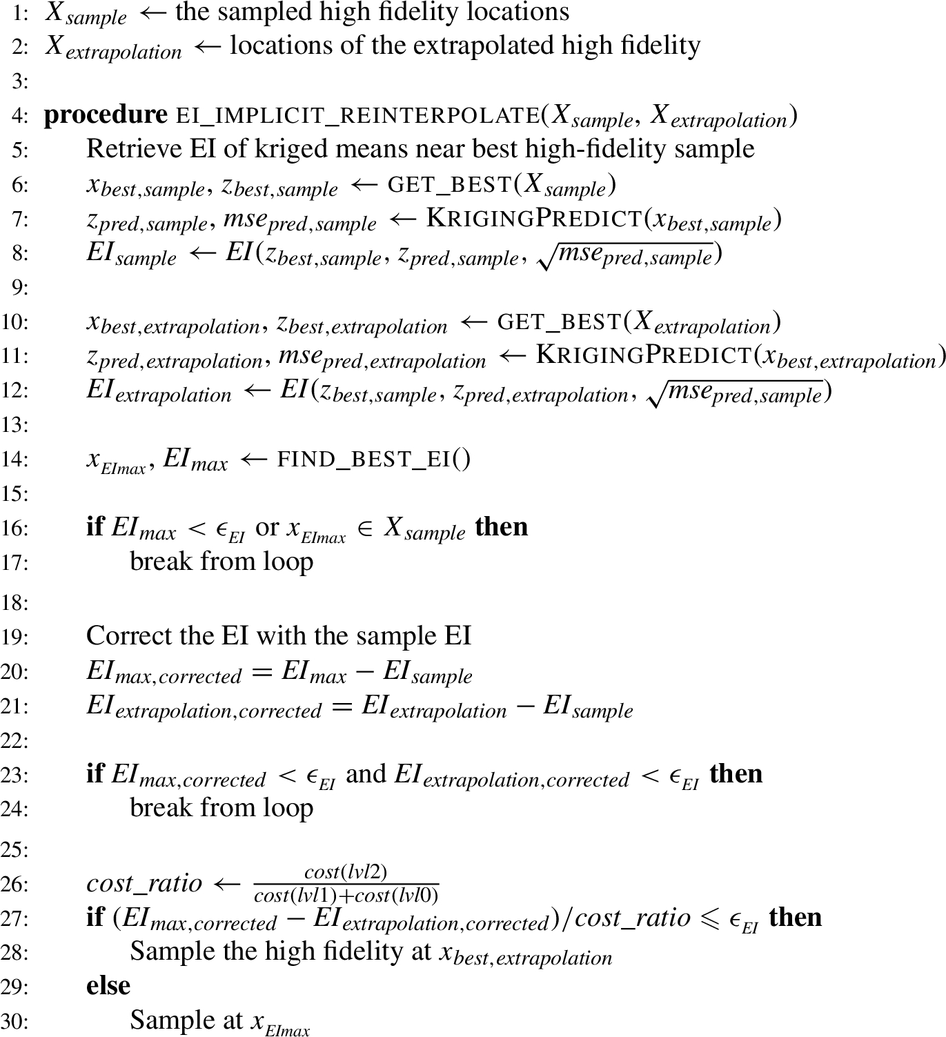
Alternative implicit EI reinterpolation procedure, fit for the proposed method

Algorithm 2 ensures that the next sampling location does not automatically default to the maximum EI location, but occasionally samples the location of the best extrapolation instead.

It does so either when the EI at the extrapolation location is higher than the maximum EI, or the difference between these two options normalised with the involved maximum expected cost ratio is lower than the criterion ${\mathit{ϵ}}_{\mathit{EI}}$ .

At the best extrapolation, the lower fidelities were already sampled and so the high fidelity will be sampled next. The used cost ratio is therefore calculated as the cost of the high fidelity over the minimal cost of sampling at the location of maximum EI, which in this case is the cost of (nested) sampling the lower fidelities.

Algorithm 2 ensures that we do not sample the lower fidelities at infinitesimally small intervals, but sometimes sample the higher fidelity to lower the actual non-corrected Expected Improvement.

Compared to the original reinterpolation routine of Forrester et al. [7] the surrogate does not have to be retrained. The routine of Algorithm 2 is thereby about half the computational cost.

Algorithm 2 is in effect near identical to the original reinterpolation routine of Forrester et al. [7] if there are no extrapolations present. The Expected Improvement of samples is pushed to a maximum of 0. The primary difference is believed to be found in the evaluation of the Kriging variance, between samples, since the variance at the samples influences the process variance that is solved for during the hyperparameter optimisation. However, in that regard, the procedure proposed here should be regarded as the more accurate method that is more true to the Kriging model.

2.7. Implementation details

The proposed method is dependent on accurate noise estimates to provide results as desired. This observation involves some considerations in the method implementation:

The extrapolated high-fidelity surrogate should always be decoupled from the noise estimates on the lower two fidelities. In the proposed method, the high fidelity ‘samples’ include extrapolated values, based on information of the lower fidelities. Thereby the result of the proposed method determines the value of the noise estimates it will use itself at the next timestep. This co-dependency would instigate instability in the surrogate during the course of optimisation.

Each fidelity level should be a single-fidelity surrogate. To see why this is, consider that the multi-fidelity Kriging model of Bouhlel et al. and Gratiet and Garnier [4,21] combines the fidelity levels and deducts a single process variance $\hat{\mathit{\sigma }}$ which is coupled to the regression parameter, while giving the higher fidelity information prevalence over lower fidelity information sources. The inter-dependent noise estimate of the multi-fidelity Kriging model of Gratiet and Garnier [21] aids in getting the best estimate at the highest fidelity but might not necessarily retrieve the best estimate for a lower fidelity in isolation, especially when the MFK methodology is less applicable. For example, a low $\hat{\mathit{\sigma }}$ as might be indicated by higher-fidelity data will retrieve a higher noise estimate if the process variance is in fact naturally higher at that lower fidelity level. The proposed method benefits from unbiased noise estimates, and so each lower fidelity should be a single-fidelity model.

When using a reinterpolation routine for EI calculation, one should take care that the reinterpolation does not affect the lower fidelities.

It is beneficial to the proposed method to sample the lower fidelities at locations directly around higher fidelity samples to get better noise estimates and thereby a more stable Kriging mean. Without doing this, it might be that the extrapolated surrogate is quite unstable during optimisation until an area in the design space emerges that is more densely sampled. Doing the same does not provide an advantage to the reference method [21,26], so rather than instigating an unfair advantage, acquiring these additional lower fidelity samples is a disadvantage in terms of costs for the proposed method.

Just as the proposed method benefits from unbiased noise estimates per fidelity level, the same is true for the Kriging means that are used to extrapolate. The Kriging mean should be regarded as the surrogate that is corrected for noise in the input data. This is as well the reason why the extrapolation is based on the Kriging mean and not on the original data, with a clear difference present in the performance of the proposed method.

Code for the proposed method is available at https://github.com/robertwenink/MFK-Extrapolation.

3. Design simulation setup

Realistic test scenarios where the data is acquired by means of CFD simulations using the CFD solver described in Eijk and Wellens [40]. The design problem will consist of only two actively controlled variables. This is due to three reasons:

• We are verifying a novel method using a CFD evaluation function fit for maritime engineering purposes. Issues are harder to pinpoint for higher-dimensional design problems.

• Visualisation of two-variable response surfaces is relatively straightforward and less confusing compared to higher dimensional problems.

• The used CFD solver has been under development in 2D until now. Sensible one-to-one 2D design parametrisations with more than two variables were not found.

Since our primary aim is to validate our proposed method, we will not consider multi-objective or constrained formulations. Note that a 3D simulation tool can also be used since the objective output per simulation remains a scalar, see Eq. (18). Furthermore, the proposed method is applicable to higher dimensional design problems, keeping in mind that the effectiveness of the proposed method is primarily dependent on the validity of the main assumption.

In the following the test case and the objective function will be elaborated upon, the parametrisation used to define one-to-one shape variations will be described, and, finally, the filtering procedures to remove errors of numerical origin is discussed.

3.1. Case description

The in-house CFD solver that has been used is called EVA [40–42] and developed with a focus on extreme fluid-structure interaction (FSI). EVA is a multiphase flow solver based on the 2D Navier–Stokes equations for the motion of a mixed fluid. The method uses a fixed staggered Cartesian grid on which the free-surface between water and air is described using a geometric Volume-of-Fluid (VoF) method. The interface is represented by piecewise linear line segments and transported using a direction-split scheme.

Examples of extreme FSI are found when waves impact with structures [2,29,42,44,45]. Note that when waves are concerned, simulations benefit from Generating Absorbing Boundary Conditions [5,6], both in terms of accuracy and of computing time. Slamming of an object onto a free water surface constitutes another type of impact simulation, demonstrated by means of a falling cylinder on water in van der Eijk and Wellens [40].

A well-known 2D test case for such impact simulations is the ‘free-falling wedge’ which in our case mimics the collision with water of a free-fall lifeboat: a rescue vessel that drops off an offshore drilling platform into the sea in case of emergency. After the rescue vessel slams the water, constituting the moment with the highest vertical accelerations, flow separation and the generation of a cavity follows. EVA [40] has been validated for the whole entry procedure.

The deformation capacity of the falling object itself, as in Bos and Wellens [3], Xu and Wellens [47,48], is not taken into account, and the object is considered completely impermeable and not porous [44]. We will modify the scenario with a 2D falling wedge to represent a single-objective optimisation problem in which we vary the shape of the falling life boat’s nose or ‘bottom’ in the way that we have set up the simulations.

The optimisation objective is to minimize the maximum acceleration of the wedge as the main indicator for the immediate safety of its hypothetical passengers: $$\begin{array}{}\text{(18)}& {\mathit{y}}_{\mathrm{opt}}=\underset{\mathit{x}\in \mathit{X}}{min}\mathrm{(}max\mathrm{(}{\mathit{a}}_{\mathit{x}}\mathrm{)}\mathrm{)}\end{array}$$ Here, ${\mathit{a}}_{\mathit{x}}$ denotes a time trace of accelerations, at location x within the full domain X. The max operator is applied to the accelerations of the life boat in the simulations, whereas the min operator is applied on all accelerations in all simulations, the minimum of which is considered optimal.

Fixed parameters in this problem will be:

All environmental constants, such as gravitational acceleration $\mathit{g}=9.81$  m/s and water density ${\mathit{\rho }}_{\mathit{w}}=1025$  kg/m³.

Main dimensions of the boat: the size in beam direction $\mathit{B}=3.4$  m is the main dimension that will lead to obstruction of the flow around the structure upon impact with the free surface; the size in draft direction $\mathit{D}=4.3$  m is the out-of-plane dimension when the free-fall life boat is assumed to fall completely vertically (high mass case). The length $\mathit{L}=12.6$  m of the boat is the out-of-plane dimension when evaluating the hypothetical scenario that the free-fall life boat impacts the free surface bottom-first (low mass case).

Mass or the loaded weight of the boat $\mathit{M}=15\mathrm{,}816$  kg

The height of the boat’s bottom shape variations $\mathit{h}=\mathit{D}\mathrm{/}2=2.15$  m.

Design dropping height $\mathit{H}=36$  m, equivalent to the frictionless free-fall impact velocity $\mathit{v}=26.58$  m/s ( $=95.68$  km/h).

All capitalized constants are based upon a real offshore free-fall boat.3

³

https://www.palfingermarine.com/en/boats-and-davits/life-and-rescue-boats/free-fall-lifeboats#anchorslides_content_contentslides11_5; model: FF 1000 S M2; visited 20/06/2023.

The mass will be varied between different optimisations (but fixed per optimisation problem) since it is interesting to observe its effect. For instance, a vessel with low mass and thus low specific weight compared to the water might benefit from a more axe-shaped bottom, because buoyancy or added mass effects might de-accelerate the vessel before the primary impact. On the contrary, a vessel with a high mass and thus high specific weight would slow down much less and would benefit from avoiding anything close to flat-plate impacts.

Furthermore, from a design perspective, it makes more sense to fix the mass than for instance to fix the mass-buoyancy ratio or specific weight of the vessel. This is because the main dimensions, required load capacity, and structural weight are more or less already fixed.

We will consider the following two masses in these experiments, where one should note that the 2D CFD solver EVA accepts a mass per meter:

• $\mathit{m}=\mathit{M}=15\mathrm{,}816$  kg/m. This scenario with high mass per meter represents a more realistic scenario in which the lifeboat collides with the water with its length perpendicular to the water’s surface.

• $\mathit{m}=\frac{15\mathrm{,}816}{12.6}=1\mathrm{,}255$  kg/m. This scenario with a low mass per meter coincides with the lifeboat colliding with the water over its full length at once, parallel to the water’s surface. This is not necessarily a realistic scenario but is a case variation that could be interesting to optimise nonetheless.

Since we have fixed the mass per design optimization in our experimental setup, the optimization objective acceleration is proportional to the surface-integrated body forces in the vertical y-direction.

3.2. NURBS parametrisation

The parameters which determine the shape of the wedge’s bottom spline are the parameters that define the domain of the surrogate model. We will use Non-Uniform Rational B-Splines (NURBS) to define this shape, see Piegl and Tiller [31] for extensive information. NURBS are implemented in the geomdl python package [1].

We impose some constraints on the shape endpoints:

• The angle of the spline at the bilge is constrained between 10 degrees (horizontally inward) and 90 degrees (vertically down)

• The angle of the spline at the keel is constrained between 10 degrees (horizontally outward) and 80 degrees (up).

Both horizontal 10-degree angle restrictions are in place to prevent situations too close to flat-plate impacts, which are numerically hard to simulate. Further, we consider an angle of 90 degrees vertically up at the keel to be unrealistic and not physically constructible and likewise restrict it to (90 −10) = 80 degrees.

We will limit the dimensionality of the design problem to 2. Note that normally by using NURBS, shapes such as the flare bow [50] can be created. Likewise, if we do not impose topological constraints on the vertical location of the control points, we can arrive at catamaran-like shapes. These would provide an interesting class of shapes involving air entrapment. However, proper optimisation requires a one-to-one shape parametrisation, meaning that each input x retrieves a unique shape. Simultaneously, we are limited to 2D shape variations due to the development status of EVA [40]. In 2D, we did not succeed in attaining a one-to-one parametrisation when including the above interesting variations while retaining the simpler but nonetheless important shape variations. Especially triangular bottom shapes were commonly constructed by non-unique and completely different inputs. We choose to retain only the simpler and more interpretable shape variations, defined purely by the angular constraints above.

Because we are interested in the primary impact response and not necessarily in any buoyancy effects after the bilge has submerged, we decrease the freeboard to only 0.5 m to decrease the numerical domain size.

Given a NURBS shape parameterisation, a resulting body is exported to an image. From this image, an SDF (Signed Distance Function) is created, providing the shortest distances to the body boundary where negative values are inside the body and positive values are outside the body. This SDF function is then used to project a body-fraction field upon the simulation grid corresponding to the shape of the provided NURBS image. Lastly, based on this fraction field the body is reconstructed in the grid using the Piecewise Linear Interface Calculation technique.

An example result of the mapping of a NURBS parameterisation to a reconstructed body in-grid is provided in Fig. 2.

Fig. 2.

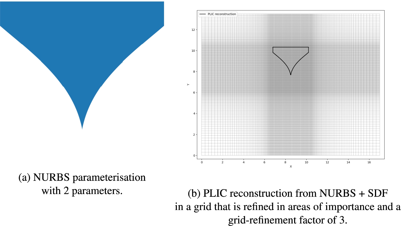
NURBS input image (a) and reconstructed output (b) for X = [06975, 09443].

3.3. Definition of the numerical grid and the fidelity levels

The definition and coarseness of the numerical grid directly influences the accuracy and costs of the simulation and thereby determine the effective fidelity level. Therefore, first the grid definition is provided, followed by a description of how that grid is refined to create the required fidelities.

The grid definition has to conform to some requirements or preferences:

• It has to be symmetric over the body, effectively meaning we require an even number of grid cells for a body defined at the centre of the x-axis.

• In height and especially in the width, any grid-cell boundary cannot perfectly overlap with a body boundary. In such a case, PLIC (Piecewise Linear Interface Construction [49]) cannot reconstruct that body boundary, instigating numerical problems. This is true for the definition of the body of water too. It suffices to pick cell spacings that do not exactly divide the body’s main dimensions.

• To focus computational effort, the grid is defined such that the grid area that contains the body is of a higher grid density than the surroundings where no direct interactions between body and liquid occur. This area of grid refinement should encompass the whole body from the beginning to the end of the simulation and be somewhat wider to accurately capture, for instance, generated waves. Outside these defined bands of higher cell-density, the dimensional size of each consecutive cell is stretched with a factor of 1.05 as compared to its predecessor.

The standard grid definition in the computational domain resulting from these considerations is given by Table 1.

Table 1

Numerical domain size, the definition of the focussed grid area per dimension, and the corresponding effective cell-spacing

Dimension	Full domain size	Focussed grid area definition				Effective cell-spacing
		From	Until	Total size	Number of grid-cells in band
x	17.0 m	6.5 m	10.5 m	4.0 m	44	${\mathit{d}}_{\mathit{x}}=0.09091$  m
y	13.5 m	6.0 m	10.5 m	4.5 m	48	${\mathit{d}}_{\mathit{y}}=0.09375$  m

The definition of ‘refined’ grids and fidelity levels are simple but important, so will be provided separately here.

The refined grids or grid refinements adhere to the same rules as the standard grid definition provided earlier. Of particular importance is that the refinement does not break the grid symmetry around the rigid body. The standard grid definition provided above is from hereon referred to as ‘refinement factor 1’.

A refinement factor 2 takes the standard grid definition (refinement factor 1) and multiplies the number of cells within the focussed band of cells by a factor 2. In such a way we would retrieve a number of cells within the focussed grid area as given in Table 2.

Table 2

Characteristics of the focussed area in the simulation grid for a selection of refinement factors

Refinement factor	0.5	1	1.5	2	3	4
#cells in x-band	22	44	66	88	132	176
#cells in y-band	24	48	72	96	144	192
Total #cells in focus area	528	2112	4752	8448	19008	33792
dx within x-band	0.18182	0.09091	0.06061	0.04545	0.03030	0.02273
dy within y-band	0.20455	0.09375	0.06250	0.04688	0.03125	0.02344

The seemingly arbitrary usage of refinement steps of 0.5 originates from the fact that the given base grid definition uses a grid coarseness at which the simulation output seemed to be with reasonable levels of noise, provided an appropriate filtering routine and a reasonable cost level. Therefore, this seemed a good medium fidelity level, which is indexed with a 1 using 0-based indexing. The three fidelity levels required by the proposed method could now be constructed using for instance the refinement factors 0.5, 1 and 4.

Given this information, the refinement for the lower fidelity was already fixed too, at ${\mathit{l}}_0=0.5$ , due to it being the only refinement below refinement level 1 that ensures a symmetrical grid definition. Although having quite a coarse grid definition, this implies we could better expect convergence as desired while simultaneously providing us with challenging, noisy data.

The refinements used to define the fidelities for all experiments are:

1. ${\mathit{l}}_0=0.5$

2. ${\mathit{l}}_1=1$

3. ${\mathit{l}}_2=2$

These refinement levels, based upon the constant low mass scenario, are consequently applied regardless of what might be best for the other experimental scenarios. The chosen refinement level of the high fidelity is primarily based on the computation time of a CFD run. A CFD run at the lowest fidelity is completed after 1 to 3 minutes, while for the medium fidelity, this is 5 to 9 minutes. At high fidelity, a CFD run takes between 16 and 50 minutes,4

⁴

The runtimes are highly dependent on the NURBS shape provided as input. For instance, in simulations where the impact occurs with the (parts of) the body reconstruction comparatively perpendicular to the water (flat-plate impact), the required timestep is much lower and thereby the simulation times longer.

with the majority taking around 45 minutes each. CFD simulations at any refinement level higher than 2 would easily surpass a simulation time of an hour, which is deemed pragmatically infeasible during this exploratory phase of research.

3.4. CFD solver signal filtering

Having described the procedures of mapping the NURBS shape definitions onto the computational grid, we identify the need of filtering either the force signal or, equivalently, the acceleration signal retrieved by EVA such that we can retrieve a more stable objective value with a smaller error. Unfortunately, the force signal retrieved from EVA contains spikes, and these are of a purely numerical origin. Sources of these peaks are for instance the pressure peaks as described in Kleefsman et al. [16], or the PLIC reconstruction.

This custom composite filter consists of:

Filter step 1: Forward + backward time-step compensated exponential moving average. In effect, force peaks of numerical origin, occurring during small time steps, will have almost no influence on the result and thereby the next step will be much more effective.

Remove data outliers: removing data that deviates more than 8 per cent of the data mean with respect to the result of step 1, then interpolate again.

Filter step 2: Normal forward-backwards emw, with double the span to smooth result.

Filter step 2 is not necessary but improved the smoothness and correctness of the results, especially around where outliers were removed.

The results of this filtering procedure are visualized by means of a force signal in Fig. 3. In the figure, a comparison is made between the original signal and some other filters.

Fig. 3.

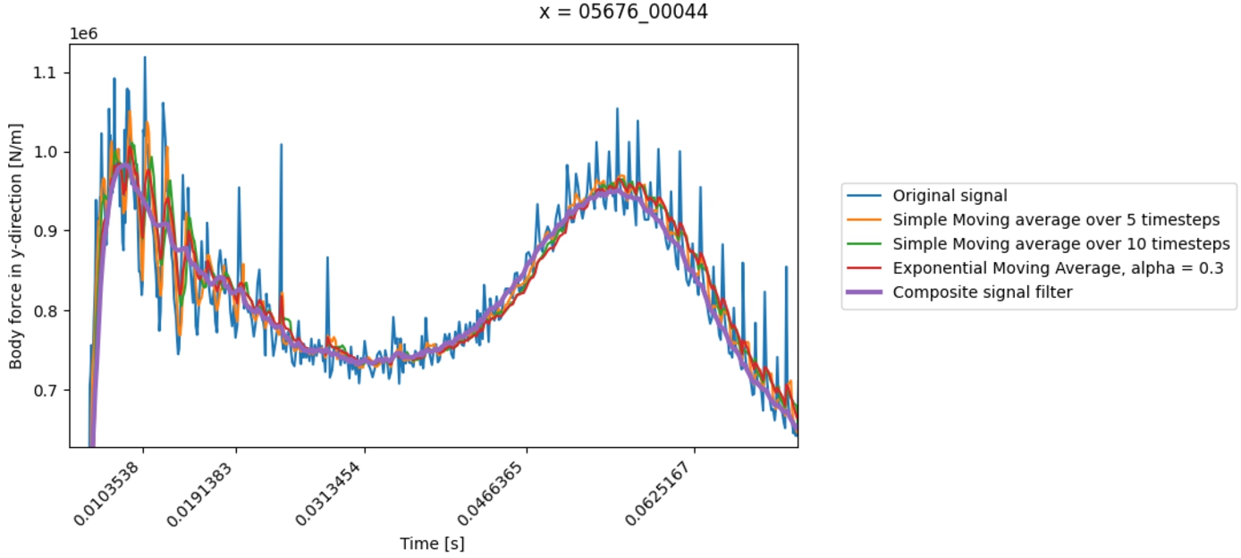
Comparison of filters. Zoom of the signal for the best design of the high mass scenario with $\mathit{m}=15\mathrm{,}816$  [kg/m]. The filtered result is more stable and not biased towards the force spikes that have a purely numerical origin like the other filtering methods are. By disregarding these spikes, the filtered result more accurately follows the actual trend of the data.

3.5. Considerations of the simulation setup

Results will be compared to the surrogate modelling method of Gratiet and Garnier [21], extended with the level selection procedure of Meliani et al. [26] in order to be used in MF-SBGO. As stated above, these methods will jointly be referred to as ‘the reference method’. The reference method has a low-fidelity level and a high-fidelity level. Note that the method proposed here, compared to the reference method, uses an additional fidelity level. A lower fidelity level was added so that that becomes the low-fidelity level in our proposed method. The original fidelity levels in the reference method will hence be referred to as medium-fidelity and high-fidelity levels in the proposed method. The other main difference with the reference method is that the proposed method features the assumption of uniform proportional grid convergence throughout the design space.

To provide a comprehensive comparison, the following metrics will be employed to offer insights into both the surrogate and SBGO methodology in terms of the costs, performance, and other underlying factors:

• The best found objective value, together with the corresponding location in the parameter-space, given by the NURBS-parameters ${\mathit{x}}_0$ and ${\mathit{x}}_1$ that describe the outer geometry of the falling wedge)

• Sampling costs, given as the total sampling cost and the high-fidelity sampling cost.

• The number of high-fidelity and low-fidelity samples.

• Normalized RMSE of the optimisation’s solution with respect to a fully sampled (initial) DoE at the highest fidelity, see Eq. (20). These are given for the high-fidelity at the start and end of a simulation, and the medium fidelity at the end of the simulation. The medium fidelity is reported as a reference that the (extrapolated) high-fidelity at the very least should outperform.

Performance is measured by comparing the predicted value with the real sampled results by using the Root Mean Squared Error (RMSE) as done in Toal [39]: $$\begin{array}{}\text{(19)}& \mathrm{RMSE}=\sqrt{{\displaystyle \frac{1}{\mathit{n}}}{\displaystyle \sum }_{\mathit{i}=1}^{\mathit{n}}{\mathrm{(}{\mathit{y}}_{{\mathit{e}}_{\mathit{i}}}-{\mathit{y}}_{{\mathit{c}}_{\mathit{i}}}\mathrm{)}}^2}.\end{array}$$ However, we prefer the normalised RMSE for better comparison between different optimisation cases: $$\begin{array}{}\text{(20)}& \mathrm{NRMSE}={\displaystyle \frac{\mathrm{RMSE}}{max\mathrm{(}{\mathit{y}}_{\mathit{e}}\mathrm{)}-min\mathrm{(}{\mathit{y}}_{\mathit{e}}\mathrm{)}}}\end{array}$$ The NRMSE will be reported as a percentage. RMSEs are calculated using the high-fidelity ‘truth’ sampled on the full initial DoE ${\mathit{y}}_{\mathit{e}}$ , where subscript i indexes such that high-fidelity samples used in the surrogate model are excluded to prevent a bias for surrogate models that use a lot of high-fidelity samples.

Random number generators are used in many aspects of the code:

The initial sampling LHS experimental design within the design space.

The LHS used in the EI maximisation sub-routine.

All these random states are set to be constant or structurally varied using counters. Thereby, although semi-random noise is applied, the simulations themselves are completely deterministic. That is, one can re-run the same simulation input and get the same results. This does however not mean that the same input x always retrieves the same result.

4. Results

4.1. Optimisation metrics and evaluation of the main assumption

Table 3

Optimisation metrics for the falling offshore lifeboat cases with the proposed method and the reference method [21,26]. The number after the used method indicates the number of initial high-fidelity samples used. The best results per scenario and metric are highlighted in bold

Scenario	Method	Method weighing	Objective		Sampling cost [-]		Number of samples [-]		NRMSE [%]
			Value [ms−2]	Location [-]	Total	High	High	Low	High (start)	High (end)	Medium (end)
Lifeboat m = 15,816 [kg/m]	Proposed 1	MFK/mf	63.59 (6.48 g)	[0.598, 0.033]	23074.72	4331.08	2	26	6.4943	8.7362	6.1023
	Proposed 3	-	63.59 (6.48 g)	[0.598, 0.033]	34355.11	12105.3	6	34	6.6711	6.3117	6.6747
	Proposed 3	MFK	62.15 (6.33 g)	[0.568, 0.004]	35924.36	12827.66	6	36	1.9887	6.4761	6.1113
	Reference 3	n.a.	63.59 (6.48 g)	[0.598, 0.033]	24147.27	11006.35	5	22	3.2519	22.3208	6.1858
Lifeboat m = 1,255 [kg/m]	Proposed 1	MFK/mf	214.88 (21.9 g)	[0.881, 0.521]	16007.25	1960.58	1	24	5.2116	5.2116	8.0242
	Proposed 3	MFK	214.88 (21.9 g)	[0.881, 0.521]	22768.63	6558.09	3	28	5.4931	5.4931	8.6596
	Reference 3	n.a.	214.88 (21.9 g)	[0.881, 0.521]	16667.21	7441.17	4	21	3.7576	38.3085	9.8313

Optimisation metrics for all the cases are given by Table 3, with the corresponding best-optimised designs reported by Fig. 8. The table compares the outcomes for the proposed optimisation method with the reference method [21,26] for the two main scenarios with different masses. Variations of the methods are made by using a different number, either 1 or 3, of starting high-fidelity samples.

For both the high mass ( $\mathit{m}=15\mathrm{,}816$  [kg/m]) and the low mass ( $\mathit{m}=1\mathrm{,}255$  [kg/m]) scenarios, the initial DoE has been fully sampled at each fidelity and represented in Fig. 4 and Fig. 5. These figures also show the design that is near-optimal. For each of the designs, the force as a function of time is provided at the three different fidelity levels so that it can be investigated how the designs interact with the water, and what the effect of grid refinement is. Although the optimisations themselves do not have access to the full high-fidelity level, these plots provide context to the optimised designs and insight into the overall convergence behaviour of EVA and the problem at hand.

Fig. 4.

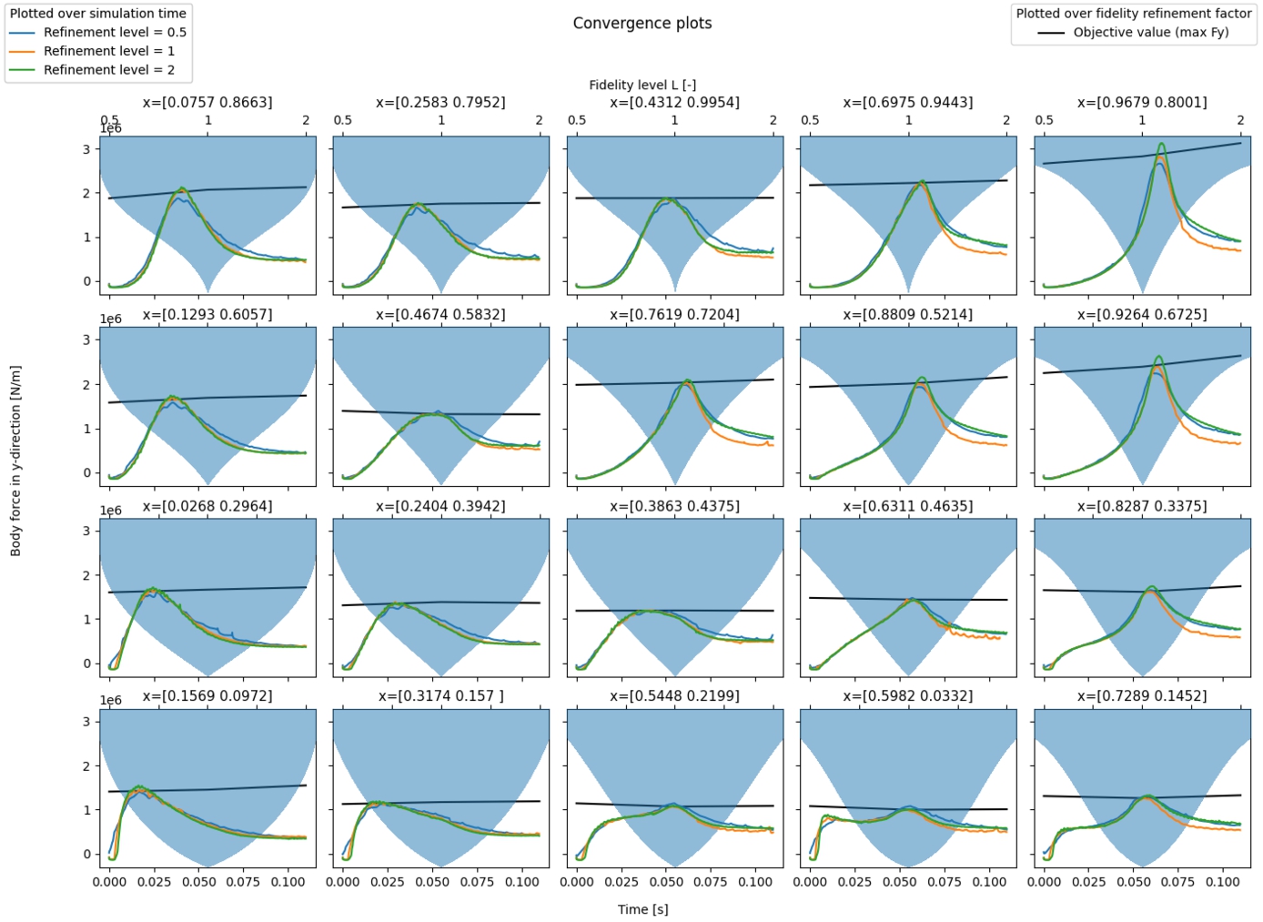
Convergence for the falling wedge experiment with $\mathit{m}=15\mathrm{,}816$  [kg/m] on the initial DoE of size 20 and over the refinement levels 0.5, 1 and 2. The black line plots the optimisation objective over the fidelity levels while the coloured lines provide the full CFD simulation time traces. The design for each NURBS parameterisation x is shown in the background. The design at x = [0.5982, 0.0332] is near-optimal.

The proposed method relies on the convergence of the objective value over fidelity levels – as stated in the main assumption. This convergence was assumed to be uniform across the design space. The validity of this assumption is inspected before analysing the optimisation results. When we look at Fig. 4 and Fig. 5 it is seen that there is the anticipated convergence at badly performing designs (large acceleration), but almost no convergence at well-performing designs (low acceleration). The observation is that CFD simulations near the optimum design will encounter less strenuous circumstances with lower forces, pressures, fluid velocities and accelerations present. Because the flow variables for these designs have lower values overall near the optimum designs, good estimates of these flow variables are already achieved at lower grid resolution. Therefore, we observe less convergence of the objective value for better designs.

Fig. 5.

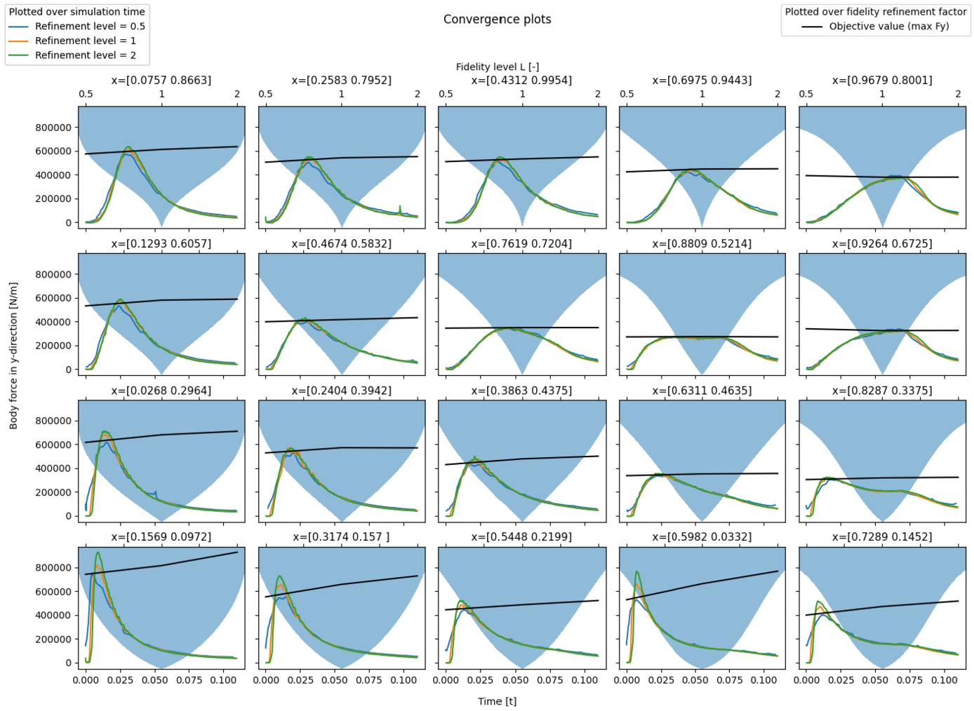
Convergence for the falling wedge experiment with $\mathit{m}=1\mathrm{,}255$  [kg/m] on the initial DoE of size 20 and over the refinement levels 0.5, 1 and 2. The black line plots the optimisation objective over the fidelity levels while the coloured lines provide the full CFD simulation time traces. The design for each NURBS parameterisation x is shown in the background. The design at x = [0.8809, 0.5214] turns out to be ‘optimal’, i.e. causes the algorithm to stop because the stopping criteria have been met.

4.2. High mass case and the low mass case

The end-states of the surrogate of the proposed method and the surrogate of the reference method [21,26] are plotted and visually compared to the ‘truth’ surrogate that is based on a fully sampled DoE at the high-fidelity in Fig. 6 for the high mass case with $\mathit{m}=15\mathrm{,}816$  [kg/m]. Figure 7 shows the same for the low mass case with $\mathit{m}=1\mathrm{,}255$  [kg/m].

Fig. 6.

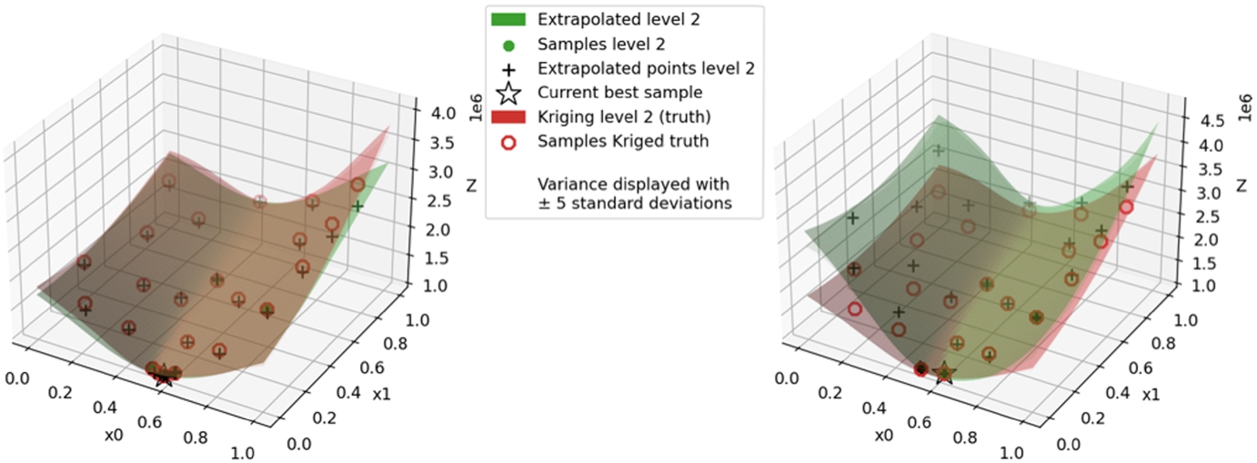
Visualization at the optimisation end of the high mass case with $\mathit{m}=15\mathrm{,}816$  [kg/m]. On the left: the proposed method with 3 starting high-fidelity samples + MFK optimisation that was able to find a better design than all other setups. On the right: the reference method, which ends with a high NRMSE due to a wrongly build trend model for the additive differences. More high-fidelity samples in the initial DoE might decrease the issue.

Fig. 7.

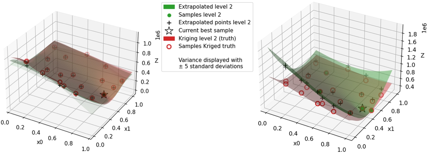
Visualization at the optimisation end of the low mass case with $\mathit{m}=1\mathrm{,}255$  [kg/m]. On the left: the proposed method with 1 starting high-fidelity sample + MFK optimisation that has all the best cost statistics and the best ending NRMSE. On the right: the reference method, which like the high mass case ends with a high NRMSE.

Figure 6 reveals the following for the high mass case. In testing the method weighing procedure, the medium fidelity is not used if the MFK solution is available, which is from 3 starting high fidelity samples and on. The problem with using the medium fidelity as the alternative surrogate is that it is not principally a solution interpolating with the high-fidelity. Although the high fidelity is forcibly added and there is in this case typically barely any difference between the high and medium fidelity in areas where the proposed method does not work well and so method weighing is used, differences over short distances could be relatively large and thus noise estimates overestimated.

For the case where instead the surrogate modelling method of Gratiet and Garnier [21] provides the alternative surrogate, we are ending with a higher NRMSE, similar to the experiments with the reference method [21,26], even though starting with a very accurate surrogate. When comparing the time traces of the NRMSE together with the weighing variables ${\mathit{w}}_{\mathit{i}}$ over time, we observe that as we sample more high-fidelity samples, there is a heightened probability of hitting ‘no convergence’ areas and thus likely falling back to the alternative method. At the same time, the reference surrogate provides increasingly bad results when sampling the area near the optimum. This was not expected given a Pearson correlation of 0.990 which normally implies the reference is effective [39].

Continuing on this, the simulation start of the proposed method with MFK as the alternative surrogate knows a very low NRMSE. This coincides with the reference method having good accuracy at the start too. The proposed method already applies method weighing at the simulation start, and it seems we retrieve a result that takes the best of both worlds. On top of that, this is the only optimisation run that retrieves a better design. This shows the idea of method weighing can be beneficial.

Fig. 8.

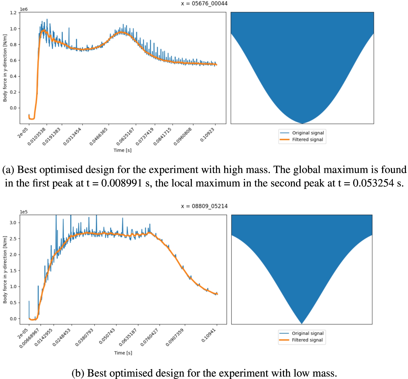
Best results of the wedge optimisations with (a) constant low mass (b) constant high mass. Next to the found optimal shape, the figures provide the body forces in the y-direction for the original acceleration signals and the signals after filtering. Although we minimise the maximum acceleration, the body forces in the y-direction are given because 1) constant body masses are used and so the translation to acceleration is the same for each point in the design space, and 2) this provides insight into how the body mass influences the involved forces whereas Tab. 3 does not.

Figure 8a shows the force on the optimal high mass case design as a function of time, and the optimal design itself. Contrary to expectations, the bottom end of the design is somewhat blunt, starting with a low gradient near the nose, after which the gradient of the cross-section increases before it becomes lower near the sides. Considering the hydrodynamics of water jet formation and jet seperation from the sides of the wedge, that is associated with the force on the wedge becoming lower, this design makes perfect sense: the design tries to avoid a single high force peak by postponing jet separation for as long as possible with a more constant force over time as the outcome.

The body forces of the best-optimised low mass design, given by Fig. 8b, are seen to be stable around the maximum value for most of the impact time, which indicates this is a very good design where we cannot expect to gain more by reducing force peaks. The design maintains a constant deadrise for most of the height of the bottom before tapering off to a more horizontal end at the chine. The peak of the low mass case force is nearly an order of magnitude lower than the high mass case force peak.

While interpreting the objective values of the low mass scenario, one should consider that due to the 2D nature of EVA used the wedge or ‘lifeboat’ effectively drops onto the body of water over its full length at once. This results in much higher forces and accelerations compared to the high mass scenario of $\mathit{m}=15\mathrm{,}816$  [kg/m]. Again, as with the high-mass case, there is low to no convergence around the optimum design.

4.3. Cost-efficiency

The objective of the proposed method is also to lower the costs of building an accurate surrogate and optimise using it, by lowering the required number of samples at the expensive high fidelity. To assess if successful, Table 3 considers the following main metrics:

• Surrogate accuracy, given by the NRMSE of Eq. (20)

• Sampling cost

For the sampling cost, it should be taken into account that the ‘low’ fidelity in Table 3 consists of only the medium fidelity for the reference method [21,26] and both the low- and medium-fidelity for the proposed method. Next to this, to improve the proposed method’s stability, extra samples around the high-fidelity samples are acquired to improve the initial noise estimates per fidelity level. Therefore, any gains by the proposed method at the high fidelity need to offset the sampling costs of the complete lowest fidelity to perform better than the reference method. The proposed method is able to do this for the simulations starting with a single high-fidelity sample.

In terms of surrogate accuracy expressed in the NRMSE, the proposed method gives comparable results to the reference method [21,26], but cannot be said to perform better. It is found to be more stable during the course of EGO optimisation. Given the nature of the problem, the reference seems to need more high-fidelity samples in the initial surrogate to perform well.

Because of the instability of the reference method and the corresponding upward parabolic surrogate, the reference might decide earlier than the proposed method to stop the optimisation based on the Expected Improvement criterion. The reference method might therefore seem to be more efficient in costs than it deserves in these scenarios.

As for the optimisation result, only the proposed method has been able to find a better design, for the high-mass case. More investigation is required to determine whether this is due to a structural strength of the method.

5. Conclusions

The main research objective was to leverage the grid convergence property of CFD solvers to reduce the number of expensive high-fidelity samples required for an accurate (multi-fidelity) Kriging surrogate, thereby accelerating surrogate-based global design optimisation in maritime engineering.

A multi-fidelity method was proposed and tested using computational experiments. The proposed method uses three fidelity levels and assumes that the differences between them are proportional across the design space to extrapolate the high-fidelity data from one point in the design space to another. It then uses the statistics and correlations of the underlying Kriging models to balance or correct the surrogate. An adapted sequential sampling and fidelity-level selection procedure was formulated such that the proposed surrogate can be used in multi-fidelity surrogate-based global design optimisation (MF-SBGO).

To investigate the possible usefulness of the proposed method to SBGO in the field of maritime engineering, the proposed method was tested by optimising the shape of two variations of a falling wedge case as an example of slamming, of which the relevance to maritime engineering is explained by Eijk and Wellens [40], using their CFD solver EVA that is tailored to the problem. The performed optimisations found two different designs of the bottom shape depending on the specific weight of the wedge, where the interplay of hydrodynamic effects resulted in non-trivial designs. In many of the considered cases, the optimal design was also found with fewer high-fidelity samples than the reference method [21,26]. However, the cost of finding the optimal design by means of the proposed method was not lower than that of the reference method in all of the cases. The main explanation is that the grid convergence of EVA was not uniform in magnitude over the design space. Near optimal designs, due to how EVA represents the hydrodynamics of slamming work, good predictions of the wedge’s acceleration were already reached at the low-resolutions, low-fidelity levels, so that information of the grid convergence obtained from other samples farther away from the optimum design was less beneficial than originally assumed. Future work will take this property about grid convergence near optimal designs into account.

Funding

This research was partially supported by Epistemic AI (964505) and by TAILOR (952215), projects funded by EU Horizon 2020 research and innovation programme.

Conflict of interest

P.R. Wellens and M. van der Eijk are Editorial Board Members of this journal, but were not involved in the peer-review process nor had access to any information regarding its peer-review. The authors have no other conflicts of interest to report.

Author contributions

R. Wenink had access to the data and was involved in: conception; performance of work; interpretation of data; writing the article.

M. van der Eijk had access to the data and was involved in: conception; performance of work; interpretation of data; writing the article.

N. Yorke-Smith had access to the data and was involved in: conception; performance of work; interpretation of data; writing the article.

P.R. Wellens had access to the data and was involved in: conception; performance of work; interpretation of data; writing the article.