Sage Journals: Discover world-class research

Abstract

Propeller performance greatly influences the overall efficiency of the turboprop engines. The aim of this study is to perform a propeller blade shape optimization for maximum aerodynamic efficiency with a minimal number of high-fidelity model evaluations. A physics-based surrogate approach exploiting space mapping is employed for the design process. A space mapping algorithm is utilized, for the first time in the field of propeller design, to link two of the most common propeller analysis models: the classical blade-element momentum theory to be the coarse model; and the high-fidelity computational fluid dynamics tool as the fine model. The numerical computational fluid dynamics simulations are performed using the finite-volume discretization of the Reynolds-averaged Navier–Stokes equations on an adaptive unstructured grid. The optimum design is obtained after few iterations with only 56 computationally expensive computational fluid dynamics simulations. Furthermore, an optimization method based on design of experiments and kriging response surface is used to validate the results and compare the computational efficiency of the two techniques. The results show that space mapping is more computationally efficient.

Keywords

Propeller design blade-element method computational fluid dynamics space mapping kriging surrogate models

Introduction

Unlike aircraft turbofan and turbojet engines, turboprop engine might be considered an old and obsolete propulsion system to be used in modern aviation industry. However, after being discarded for the years following the introduction of turbofan engines, turboprop engine is becoming a high-demand nowadays, and the attention of the research community is directed back toward it. This is because of its relatively low fuel consumption at low speeds than other aircraft engines. In addition, the vast majority of airplanes are using a propeller-based propulsion system. For instance, military, agriculture, private unmanned aerial vehicles (UAVs), and even some commercial aircraft companies are using propellers to power their aircrafts till this moment. The propeller-based propulsion system comprises mainly an engine and a propeller. Although the latter is considered the simplest part, its performance greatly affects the efficiency of the entire system. Thus, the development of this airscrew and improving its performance become of high importance.

In the literature, numerous researches have been published concerning the aerodynamic shape optimization (ASO) of an aircraft propeller blade for maximizing its efficiency. Some of them utilized the traditional blade-element theory as the aerodynamic analysis model.¹ Later studies used more advanced models^2,3 including the vortex lattice method.^4,5 Blade-element momentum (BEM) theory is the most common method employed for the preliminary design of propellers and their performance analysis. It is used either as the basic aerodynamic model⁶ or is combined with another analysis tool such as computational fluid dynamics (CFD) model.^7–11 Because of their high computational cost, CFD simulations are usually used only for analyzing or validating final design results and are less frequently used during the optimization process as in this study.

CFD is an accurate, reliable, and fundamental tool in aerodynamics. Unfortunately, its high-fidelity models might be very computationally expensive even with the advances in computer processing speeds and memory capacities. Hence, it is impractical to perform a direct optimization using these models and it is necessary to replace them with fast surrogate models. The concept of optimization via surrogate models is known as surrogate-based optimization (SBO). Such an optimization approach aims to achieve high-fidelity design optimization at low computational cost.

In SBO algorithms, the surrogate model is considered the major component. Mainly, there are two types of surrogate models: functional and physical surrogates.¹² Functional surrogates are usually based on algebraic models and can be constructed without knowing the physics of the underlying system. This type can be built using design of experiments (DOEs)¹³ to allocate sample points in the design space, followed by exploiting a data-fitting methodology. Kriging is one of the most popular data-fitting techniques. It is used to build surrogates through interpolating data obtained from DOE. Kriging-based surrogates are used in a variety of aerodynamic optimization problems such as aircraft engine nacelle design,¹⁴ axial compressor blade shape optimization,¹⁵ airfoil shape optimization,^16,17 and in marine propeller design.¹⁸ Neural networks is another technique used by Marinus et al.¹⁹ for the optimization of an aircraft propeller blade. J Carroll and Marcum²⁰ used optimal Latin hypercube (OLH) algorithm to generate initial sampling points, filling the design space and polynomial regression models for the surrogates.

On the contrary, physical surrogates are based on a previous physical knowledge of the system of interest.¹² This type is based on a low-fidelity model having the same physics of the original system but with low accuracy. This low accuracy may be a result of using the same high-fidelity model but with coarser mesh and relaxed convergence criteria,^21,22 or as a result of using a simplified physics model by, for example, neglecting three-dimensional (3D) effects as in the present study. One of the promising techniques which uses physics-based surrogates is space mapping (SM).

SM was first introduced by JW Bandler et al.²³ It is one of the most popular SBO techniques, in which the direct optimization of the high-fidelity “fine” model is replaced by iterative refinement and optimization of a physics-based low-fidelity “coarse” model. The aim of SM is to find a satisfactory solution with a minimal number of high-fidelity model evaluations.²⁴ Such a concept is used in a wide variety of fields including ASO problems such as airfoil,^25–27 and wing^28,29 design optimization, but not yet used for aircraft propeller design.

This work focuses on finding the optimum propeller blade shape using a high-fidelity analysis model with minimum computational cost. The necessity of performing an optimization of a fast, yet accurate analysis model, makes the use of SM algorithm to couple BEM theory with CFD simulations well suited for our purpose. A MATLAB code, based on BEM theory is implemented and validated using JBLADE software,³⁰ was to be used as the fast coarse model. However, ANSYS Fluent commercial software is used to perform the computationally expensive fine model simulations. An SM algorithm is then used to construct a surrogate model combining the speed of BEM theory with the accuracy, to some extent, of CFD simulations. The SM algorithm continuously updates and re-optimizes the surrogate model in an iterative manner till a matching between the coarse and fine models is achieved within an acceptable tolerance. Another methodology is utilized for validation and comparison. It is based on sampling the design space by means of DOE and generating kriging-based response surface to be then optimized.

Design problem formulation

The function of the propeller is to convert the engine power into useful propulsive force. During the propeller rotation, the airflow passing through the blades generates an aerodynamic force which can be resolved into thrust force (T) and resisting torque (Q). Efficient propellers are those providing maximum thrust with minimum torque. Our objective is to find the optimum blade geometry for maximum propeller aerodynamic efficiency.

Design variables and preassigned parameters

The quantities which affect the propeller aerodynamic efficiency (η) can be divided into two categories: preassigned parameters and design variables. The former group includes those parameters which are fixed during the optimization process. In this study, the fixed parameters are as follows: the number of propeller blades (B), propeller diameter (D), propeller rotational speed (rpm), aircraft velocity (V_∞), air density (ρ), air viscosity (μ), and the advance ratio (J) which is given by equation (1). Table 1 presents the values of these fixed parameters. For simplicity, the cross-sectional airfoil is also kept fixed along the blade radius. The standard Clark Y airfoil is chosen in this study

J = \frac{V_{\infty}}{nD} = \frac{V_{\infty}}{(\frac{rpm}{60}) D}

(1)

Table 1.

Preassigned parameters.

B	D (m)	rpm	V∞ (m/s)	ρ (kg/m³)	μ (N s/m²)	J
3	3	1000	30	1.225	1.789E–5	0.6

On the contrary, design variables are those parameters which are varied by the optimization algorithm. Since we aim to find the optimum blade chord length and pitch angle distributions along the blade radius, our design variables are set to be the blade chord length (c) and pitch angle (β) (see Figure 1) at preassigned locations along the blade span. Two design cases are investigated in this study varying in the number of the preselected locations, hence the number of design variables.

Figure 1.

Blade chord length and pitch angle at certain cross-section.

Propeller aerodynamic efficiency

The objective function is the propeller aerodynamic efficiency (η). It is defined as the ratio between the useful propulsive power to the input shaft power supplied from the engine and is given by

η = \frac{T V_{\infty}}{Q Ω}

(2)

where V_∞ and Ω are the aircraft speed and propeller angular velocity, respectively, and they are kept constant in this study. T and Q are the propeller thrust and torque, respectively, which both are functions of the design variables

\begin{matrix} T = f_{1} (c_{1}, c_{2}, \dots, c_{n}, β_{1}, β_{2}, \dots, β_{n}) \\ Q = f_{2} (c_{1}, c_{2}, \dots, c_{n}, β_{1}, β_{2}, \dots, β_{n}) \end{matrix}

(3)

where n is the number of design cross-sections. The functions f₁ and f₂ can be obtained using the two aerodynamic models described in the next section.

Design constraints

Our optimization problem includes two types of constraints: bound constraints and inequality constraints. The constraints of the first type are determined based on a sensitivity analysis. On the contrary, the inequality constraints are specified based on a physical knowledge of the problem of concern. For example, the chord length at the blade tip section must be less than that at the mean section. In addition, the value of the blade pitch angle must be decreasing with radius as the tangential velocity is increasing.

Aerodynamic models

Several propeller aerodynamic analysis theories and models have been developed along time, varying in their levels of complexity and accuracy. The axial momentum theory developed by Rankine (1865) and later by Froude is the earliest and simplest method. Later, the blade-element theory was first formulated by William Froude (1878) and then developed by S Drzewiecki (1892). The results of these two theories were then combined into the so-called strip theory or BEM theory. Later, some numerical methods have been developed such as lifting line method,³¹ surface panel method,³² and vortex lattice method.³³ Nowadays, the most recent numerical tool widely used for analysis is CFD, where the 3D Reynolds-averaged Navier–Stokes (RANS) equations are implemented and solved iteratively to calculate the flow properties around the propeller blade. In our study, we used two models to determine the propeller performance: BEM theory, as it is the most traditional method in the field, and CFD simulations to enhance the fidelity of the design.

BEM theory

This theory is a result of combining two theories: momentum theory and blade-element theory. In momentum theory, the propeller is modeled as a thin “actuator disc” with no thickness. The propeller differential thrust dT and torque dQ are obtained by applying the conservation of linear and angular momentum, respectively, on an incremental annular area of the propeller disc. On the contrary, blade-element theory is based on dividing the blade into small elements (segments) along its span. Each of which is assumed to behave separately as a finite two-dimensional (2D) wing. At each element, the differential thrust and torque can be obtained from the differential lift and drag of this element. BEM theory is derived by equating the thrust and torque obtained from the two aforementioned theories. From the geometry shown in Figure 2, it can easily be proven that the differential thrust and torque according to BEM theory are given by equations (4) and (5), respectively.

dT = \frac{1}{2} B ρ U^{2} (C_{L} \cos φ - C_{D} \sin φ) cdr

(4)

dQ = \frac{1}{2} B ρ U^{2} (C_{L} \sin φ + C_{D} \cos φ) crdr

(5)

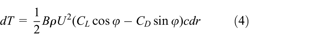
where B is the number of blades, U is the inflow relative velocity, C_L and C_D are the lift and drag coefficients, respectively, c is the element chord length, dr is the element width, and φ is the relative inflow angle.

Figure 2.

Velocity and force diagram for BEM model.

Although this model combines two theories, its accuracy is limited because it assumes that the flow around the blades is 2D. However, in reality, the flow is strongly 3D. In addition, this method also neglects the interference effects between successive blade elements. These assumptions result in errors in propeller thrust and torque calculations and consequently in performance prediction. For this reason, BEM theory is used as the coarse model in this study.

CFD

Numerical simulations of the propeller performance are based on the finite-volume discretization of the full 3D, steady, and compressible RANS equations. The governing equations relate the flow properties such as velocity, pressure, temperature, and density of a moving fluid. They are coupled with turbulence models to compute the turbulent viscosity. These fluid flow equations are discretized on an unstructured grid. ANSYS Fluent commercial Software is used to perform these simulations which are used by the SM algorithm as the high-fidelity “fine” model.

SM-based optimization

SM was originally conceived by Bandler in 1993 as a design optimization method for engineering systems. It is classified as an SBO method. The key concept of SM is to construct a surrogate model by linking a pair of available models: a low-fidelity “coarse” fast model and a high-fidelity “fine” and accordingly, computationally expensive model. The new surrogate is faster than the fine model and at least as accurate as the coarse model. The SM algorithm iteratively updates this surrogate to best match the fine model.

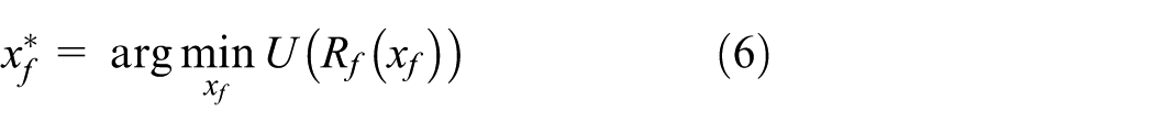
Finding the fine model optima is the main design problem which can be described by

x_{f}^{*} = \arg min_{x_{f}} U (R_{f} (x_{f}))

(6)

where $x_{f} \in R^{n \times 1}$ is the fine model design point, $R_{f} \in R^{m \times 1}$ is the fine model response vector, U is the objective function, and $x_{f}^{*} \in R^{n \times 1}$ is the fine model optimum design. Usually, the fine model is very computationally expensive to be optimized directly. SM aims to replace this direct optimization by an iterative updating and re-optimization of a surrogate model.

Parameter extraction (PE) is the main component of the SM algorithm. It is an iterative optimization process (has its own parameters), in which the surrogate model is locally realigned with the fine model. Several PE techniques were developed such as single-point (traditional) PE, multipoint PE,^34,35 statistical PE,³⁵ penalty,³⁶ and aggressive PE.³⁷ In traditional PE, a coarse model point $x_{c}$ is extracted for each fine model point $x_{f}$ to achieve the best matching between the two models. Traditional PE can be described by the following optimization problem

x_{c} = \arg min_{x_{c}} ‖ R_{f} (x_{f}) - R_{c} (x_{c}) ‖

(7)

where $R_{f}$ and $R_{c}$ are the fine and coarse model responses, respectively.

Gradient parameter extraction (GPE) is another technique which considers not only the responses but also the corresponding gradients as well,³⁸ and this enhances the uniqueness of the process. In GPE, a matching of the responses and Jacobians of both models is achieved by solving the following optimization problem

x_{c} = \arg min_{x_{c}} ‖ {[e_{0}^{T} λ e_{1}^{T} \dots λ e_{n}^{T}]}^{T} ‖, λ \geq 0

(8)

where λ is a weighting factor, $E = [e_{1} e_{2} \dots e_{n}]$ , and

\begin{matrix} e_{0} = R_{f} (x_{f}) - A R_{c} (x_{c}) \\ E = J_{f} (x_{f}) - A J_{c} (x_{c}) B \end{matrix}

(9)

Several SM concepts and techniques are reviewed and presented by Bandler et al.,²⁴ such as aggressive SM, implicit SM, and neural SM. The generalized space mapping (GSM) is another approach introduced by Koziel et al.^39,40 and is used in this study. In such an approach, the surrogate model is defined as

R_{s}^{(i)} (x) = A^{(i)} R_{c} (B^{(i)} x + c^{(i)}) + d^{(i)} + E^{(i)} (x - x^{(i)})

(10)

where

(A^{(i)}, B^{(i)}, c^{(i)}) = \arg min_{(A, B, c)} ε^{(i)} (A, B, c)

(11)

d^{(i)} = R_{f} (x^{(i)}) - A^{(i)} R_{c} (B^{(i)} x^{(i)} + c^{(i)})

(12)

E^{(i)} = J_{f} (x^{(i)}) - A^{(i)} J_{c} (B^{(i)} x^{(i)} + c^{(i)}) B^{(i)}

(13)

where $B^{(i)} \in R^{n \times n} and c^{(i)} \in R^{n \times 1}$ are the input SM parameters, and $A^{(i)} \in R^{m \times m}, d^{(i)} \in R^{m \times 1}$ and $E^{(i)} \in R^{m \times n}$ are the output space mapping (OSM) parameters. The matrices B, c, and A are obtained using PE process applied to the matching condition $ε^{(i)}$ . They are used to initially reduce the misalignment between the coarse and fine models around the current point $x^{(i)}$ . Then, matrices $d and E$ are calculated using equations (12) and (13) to ensure perfect matching of responses and first-order derivatives, respectively. The Jacobians $J_{f} and J_{c}$ of the fine and coarse models at $x_{f} and x_{c}$ , respectively can be obtained by finite difference (perturbations) if the exact derivatives are not available.

The matching condition $ε^{(i)}$ aims to align the fine and surrogate model responses and/or their first-order derivatives. A general form of this matching condition is

\begin{matrix} ε^{(i)} (A, B, c) = \sum_{k = 0}^{i} W_{k} ‖ R_{f} (x^{(k)}) - A . R_{c} (B . x^{(k)} + c) ‖ \\ + \sum_{k = 0}^{i} V_{k} ‖ J_{f} (x^{(k)}) - A . J_{c} (B . x^{(k)} + c) . B ‖ \end{matrix}

(14)

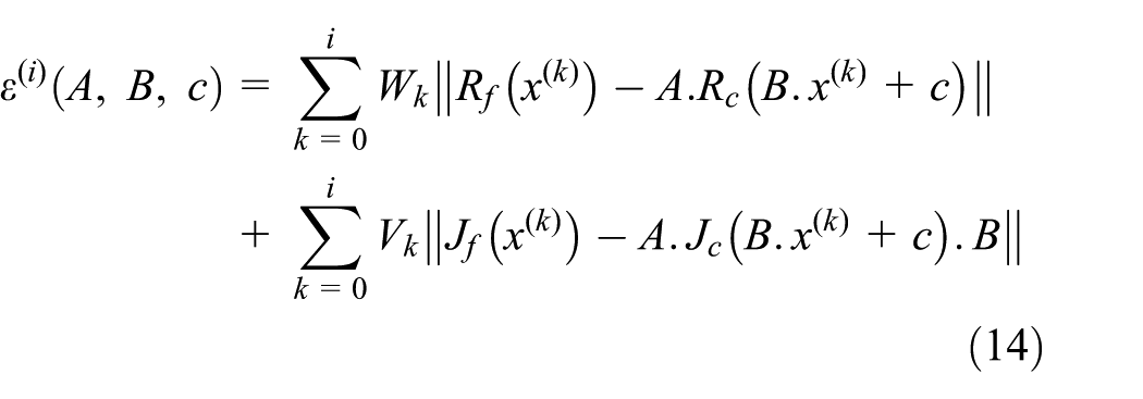
For simplicity, the coefficients $W_{k}$ and $V_{k}$ might assumed to be either 0 or 1 (though other values are possible). For example, setting $W_{k} = 1, k = 0, \dots, i$ and $V_{k} = 0, k = 0, \dots, i - 1, V_{i} = 1$ means that the algorithm tries to match the surrogate and fine model responses at all previous points including the current one, as well as Jacobian at the current point only. In this study the surrogate tries to match the fine model response and Jacobian at the last three points including the current point. A flowchart of the SM algorithm used in this study is shown in Figure 3.

Figure 3.

Space mapping flowchart.

Implementations

Coarse model

In this study, a code based on BEM theory is developed and used as the coarse model. The input parameters to this model are as follows: the distributions of the chord length (c) and pitch angle (β) along the blade radius, the aircraft speed (V_∞), the propeller rotational speed (rpm), as well as a particular cross-sectional airfoil. Given these inputs, the program goes through an iterative process to determine the induced velocities which are then used to determine the relative inflow angle φ, hence the local angle of attack α. The lift and drag coefficients, C_L and C_D, are then obtained using the airfoil characteristics. Equations (4) and (5) are used to determine the differential thrust and torque to be then integrated over the blade radius to obtain the overall propeller thrust and torque which are used, in turn, to calculate the efficiency. This program is used in conjunction with the MATLAB optimization toolbox to find the optimum blade geometry. Finding the optimum can be understood as, the problem of obtaining the optimum chord length and pitch angle distributions along the blade radius for maximum aerodynamic efficiency.

Fine model

In this study, CFD simulations are used as the high-fidelity fine model to accurately predict the propeller performance. ANSYS Fluent commercial software is used for all 3D steady simulations carried out in this study. Fluent uses, by default, second-order discretization accuracy for the viscous terms of the governing equations, while it allows the user to choose the scheme for the convection terms of each governing equation. For convection, a second-order upwind scheme is also used for the momentum equation, as it obtains more accurate results for the tetrahedral mesh used in this study. The pressure-based solver has been traditionally used for incompressible and mildly compressible flows, while the density-based solver was originally designed for high-speed compressible flows. However, both solvers are now applicable to a broad range of flows (from incompressible to highly compressible). In this study, the pressure-based solver is used since the rpm, hence velocities, is low that the flow can be assumed incompressible. Even though the flow might reach relatively high speeds near the blade tip, the solver is still applicable and there is no significant change in the results between the two solvers. In addition, we found that the pressure-based solver generally yields better convergence. Although it requires more memory, the coupled algorithm is chosen, as it significantly improves the convergence speed. The turbulence is modeled by the shear-stress transport (SST) k-ω model, since it offers some advantages relative to k-ε and the Spalart–Allmaras models, as stated in Fluent user’s guide.⁴¹ It is better than k-ε model in predicting adverse pressure-gradient boundary layer flows and separation and more accurate than Spalart–Allmaras model in predicting the details of the wall boundary layer characteristics.

Standard boundary conditions are applied on the boundaries of the computational domain. At the inlet, the velocity is assumed to be uniform, and its value is equal to the freestream velocity. At the outlet, the pressure is equal to the atmospheric pressure. The inlet boundary is placed 3 m (two times the blade radius) in front of the blade, whereas the output boundary is located 6 m (four times the blade radius) behind the blade. The geometry is larger behind the blade because we are not exactly sure how the flow will behave after interacting with the blade. Therefore, we need to have a sufficiently large volume to make sure to include all important flow behaviors. The no-slip boundary condition is applied to the blade surface to account for the flow viscosity. Since the flow around propeller is considered axisymmetric about the rotational axis, the computational domain is reduced by modeling only one blade and using periodic boundary conditions on the axisymmetric planes. The computational domain and boundary conditions used for the numerical simulations are shown in Figure 4.

Figure 4.

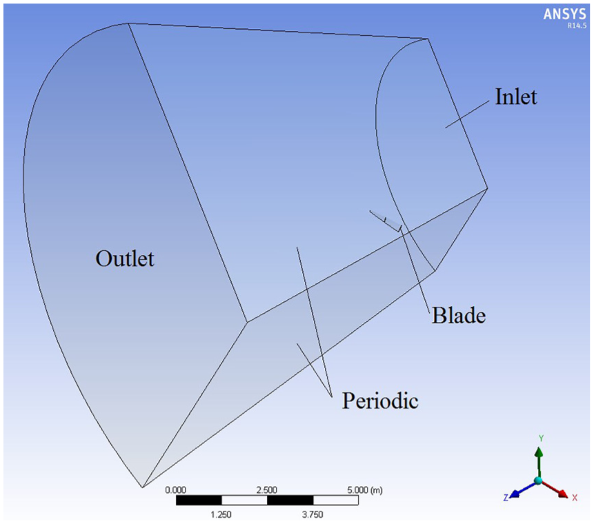
The computational domain and boundary conditions.

In general, using hexahedral mesh in the boundary layer zone to control the Y+ trend is a good way to accurately calculate the flow in this region. However, due to the complexity of the propeller geometry, tetrahedral mesh is used in this work. In addition, we controlled the mesh quality and the size of elements near the blade wall to be so small as shown in Figure 5. This also produced accurate results as indicated by the agreement of the numerical and experimental results in Figure 6. In addition, the overall mesh quality is considered very good according to the values of two mesh quality metrics. The average skewness of the elements in our mesh is about 0.233 and the average orthogonal quality is 0.857 which both fall within the outstanding range.

Figure 5.

Tetrahedral mesh around the blade: (a) mesh around the blade and (b) mesh around the blade cross-sectional airfoil.

Figure 6.

Comparison between the fine model computations and experimental results.

Mesh-sensitivity analysis

For CFD simulations, a fine mesh is important not only for solution accuracy but for allowing the computational flow to see precisely the actual geometry as well. However, very fine meshes are impractical to be used, as they extremely increase the computational time. Thus, a mesh-sensitivity analysis is performed to determine the minimum mesh size required for an accurate solution. In this analysis, the level of mesh refinement, hence mesh size, is controlled by changing the size of the grid elements near the wall of the blade as shown in Figure 5.

The optimum point of the coarse model is chosen to perform this analysis. The effect of changing the mesh size on results is studied by monitoring the variation of two output parameters: the propeller thrust and efficiency as indicated in Table 2. The results show that the thrust and efficiency obtained using a mesh size of one million elements are 99.8%, 99.6%, respectively, of those obtained using eight million elements, but with only 11% computational time. Therefore, a mesh size of one million elements is used for all simulations carried out in this study.

Table 2.

The variation of propeller thrust and efficiency with mesh size.

Number of elements (in millions)	0.25	0.5	1	2	4	8
Thrust (T)	951	960.5	987.4	987.6	989.1	989.5
Efficiency (η)	0.7452	0.7565	0.7851	0.7854	0.7906	0.7884

Validation of the numerical solution

Through its technical reports, NACA provides a huge database of experimental performance characteristics for various types of propellers. Such reports have been used by researchers to validate their propeller performance models and new formulations.⁴² To validate the CFD model, we used the 5868-9 propeller geometry.⁴³ It is a three-blade, 10-foot (about 3 m) diameter propeller of Clark Y cross-sectional airfoil. The propeller blade geometry is built and the simulations are performed over a range of advance ratios. The computed and experimental thrust coefficient and propeller efficiency are compared as shown in Figure 6. At low advance ratios, the numerical solution is in good agreement with the experimental results. However, the computed efficiency is slightly less than that of the experiments at high speeds. This might be due to the losses at the hub region, as there is no spinner modeled in our study. Spinner is that part enclosing the hub portion of the propeller and its effect can be translated into a reduction in drag at that region. Its use is more beneficial for high speeds because the drag of the hub portions of the blades is higher than for low speeds.⁴³

Comparing the coarse and fine model responses

Koziel et al.⁴⁰ stated that, “If the misalignment between the fine and coarse models is not significant, SM-based optimization algorithms typically provide excellent results after only a few evaluations of the fine model.” In addition, Bandler et al.²⁴ mentioned that, “SM techniques require sufficiently faithful coarse models to assure good results.” Thus, it is worth comparing the results (responses) of both coarse and fine models before applying the SM algorithm and starting the optimization process.

When comparing the two models, there are two aspects which mainly affect the propeller performance and need to be considered; the flight conditions at which the propeller operates and the blade geometry. The flight condition refers to the aircraft speed (V_∞) and the propeller rotational speed (rpm), and it can be represented by the advance ratio (J). Whereas, blade geometry, in this study, refers to the blade chord length and pitch angle distributions along the blade radius. Two methods were used for the aim of comparison. First, the geometry of the coarse model optimum blade is kept fixed and the responses are compared over a range of advance ratios. Second, the advance ratio is kept constant at 0.6 and the responses are compared for 30 randomly chosen blade configurations. The comparison is depicted in Figure 7.

Figure 7.

Comparison between the coarse and fine model responses.

From Figure 7, it is obvious that the coarse and fine model responses have similar trends, and they are not significantly misaligned. Therefore, it is expected that the SM optimization algorithm will obtain good results after a few iterations.

SM algorithm

An SM algorithm is used to link the two aforementioned coarse and fine models during the optimization process. The algorithm starts from an initial solution, x_i, then optimizes the coarse model to find its optimum point, x_c*. Then it solves iteratively till a satisfactory optimum fine model solution, x_f*, is obtained. At each iteration, the algorithm updates then re-optimizes the surrogate model to find a new point (optimum). The surrogate model optimum is close enough to that of the fine model if their responses (efficiency) are close enough in a region of interest. The algorithm can be summarized by the following steps:

Step 1. Set $x_{f}^{(0)} = \arg min_{x} U (R_{c} (x)) \equiv x_{c}^{*}$ , and set $i = 0$ .

Step 2. Evaluate $R_{f} (x_{f}^{(i)})$ and $J_{f} (x_{f}^{(i)})$ .

Step 3. Terminate if convergence criterion is satisfied, and set $x_{f}^{*} = x_{f}^{(i)}$ .

Step 4. Apply PE to obtain the matrices $B^{(i)}, c^{(i)}, and A^{(i)}$ .

Step 5. Evaluate the matrices $d^{(i)}, E^{(i)}$ using equations (12) and (13).

Step 6. Obtain $R_{s}^{(i)}$ using equation (10).

Step 7. Find $x_{f}^{(i + 1)} = \arg min_{x} U (R_{s}^{(i)} (x))$ .

Step 8. Set $i = i + 1$ , and go to Step 2.

Optimizing the surrogate model in Step 7 is performed by solving our constrained optimization problem using the MATLAB optimization toolbox.

Sensitivity analysis

A parameter-sensitivity analysis is performed to study how the objective function, the efficiency, is influenced by the input design variables in order to specify reasonable ranges for the design variables. The optimum point of the coarse model is chosen for the analysis, and the effect of each design parameter is studied separately by changing this parameter while keeping the rest constant. The efficiency variation with our main six design variables is shown in Figure 8. Where c₁, c₂, and c₃ are the chord length at hub, mean, and tip sections, respectively, and β₁, β₂, and β₃ are the pitch angle at hub, mean, and tip sections, respectively. It can be noticed that each design variable has a value at which the efficiency has its peak. Reasonable ranges for the design variables are chosen around these values by defining lower- and upper-bound vectors.

Figure 8.

Sensitivity analysis.

Results and discussions

As mentioned before, two cases are considered varying in the number of design parameters: (1) six design parameters where three sections along the blade span are considered and (2) 10 design parameters where 5 sections along the blade span are considered.

Case 1: three design cross-sections

In this problem, three sections along the blade radius are considered: hub, mean, and tip; each section has two design variables. Therefore, we have a total number of six design variables, $x \in R^{6}$ , as follows

x = [c_{1}, c_{2}, c_{3}, β_{1}, β_{2}, β_{3}]

(15)

where c₁, c₂, and c₃ are the chord length at hub, mean, and tip sections, respectively, and β₁, β₂, and β₃ are the pitch angle at hub, mean, and tip sections, respectively. The final distributions of the chord length and pitch angle are obtained from their values at these three locations by assuming a second-order distribution along the blade radius as shown in Figure 9.

Figure 9.

Second-order chord distribution.

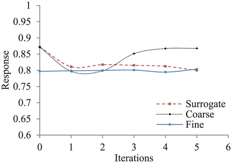
The ranges of the design variables are defined by the lower-bound vector [0.2 m, 0.15 m, 0.05 m, 30°, 15°, 0°] and the upper-bound vector [0.3 m, 0.25 m, 0.15 m, 60°, 45°, 30°] which are determined based on a sensitivity analysis. The initial solution vector x_i is set to be [0.2 m, 0.25 m, 0.15 m, 60°, 30°, 15°]. From this initial solution, the algorithm obtained the coarse model optimum point x_c* [0.3 m, 0.15 m, 0.05 m, 37°, 20°, 12°]. After seven iterations with a total number of 56 fine model simulations, the matching between the surrogate and find models is achieved, as seen in Figure 10, and the optimal solution of the surrogate model can be then assumed to be the fine model optimum point x_f* [0.2 m, 0.15 m, 0.05 m, 37°, 21°, 13°].

Figure 10.

Variation of responses with iterations.

From Figure 10, it can be noticed that the surrogate model is initially set to be the coarse model as their responses coincide at the initial (0) iteration, then the response deviates with iterations till it matches the fine model response at the last iteration. This matching is an indication that the desired fine model optimum is finally obtained. The stopping criterion of the algorithm is, thus, defined as

‖ R_{f} (x^{(i)}) - R_{s} (x^{(i)}) ‖^{2} \leq 1 \times 10^{- 5}

(16)

The convergence of the solution with iterations is illustrated in Table 3. A total improvement of 14.9% in the propeller efficiency is achieved with respect to the initial design. The isometric view of the optimum blade shape and the corresponding design cross-sections are shown in Figure 11.

Table 3.

Convergence of the solution (case 1).

Iteration	Solution vector $x^{(i)}$	$R_{f} (x^{(i)})$	$R_{s} (x^{(i)})$	$\| \| R_{f} (x^{(i)}) - R_{s} (x^{(i)}) \| \|^{2}$
0	$x_{i} = [0.2 m, 0.25 m, 0.15 m, 60^{°}, 30^{°}, 15^{°}]$	0.6970	0.7230	6.76E–04
0	$x_{c}^{*} = [0.3 m, 0.15 m, 0.05 m, 37^{°}, 20^{°}, 12^{°}]$	0.7866	0.8695	6.87E–03
1	$[0.2 m, 0.25 m, 0.05 m, 30^{°}, 23^{°}, 14^{°}]$	0.7476	0.8625	1.32E–02
2	$[0.3 m, 0.15 m, 0.05 m, 30^{°}, 20^{°}, 15^{°}]$	0.7837	0.7994	2.47E–04
3	$[0.2 m, 0.15 m, 0.05 m, 60^{°}, 20^{°}, 18^{°}]$	0.7662	0.8650	9.76E–03
4	$[0.2 m, 0.25 m, 0.05 m, 60^{°}, 22^{°}, 13^{°}]$	0.7676	0.7898	4.93E–04
5	$[0.2 m, 0.15 m, 0.05 m, 30^{°}, 21^{°}, 8^{°}]$	0.7864	0.7774	8.10E–05
6	$[0.3 m, 0.16 m, 0.05 m, 31^{°}, 22^{°}, 9^{°}]$	0.7892	0.7941	2.40E–05
7	$[0.2 m, 0.15 m, 0.05 m, 37^{°}, 21^{°}, 13^{°}]$	0.8014	0.8045	9.61E–06

Figure 11.

Optimum blade shape: (a) isometric view and (b) side view of the three design cross-sections.

Comparing the current optimal design with a NACA blade design

It is worth mentioning that the 5868-9 propeller tested in NACA report no. 658⁴³ has a similar pitch angle distribution as the current optimum design, but with a different chord distribution. Table 4 illustrates the difference.

Table 4.

Current blade versus NACA blade.

	x₁	x₂	x₃	x₄	x₅	x₆	η
Current blade	0.2 m	0.15 m	0.05 m	37°	21°	13°	0.8014
NACA blade	0.11 m	0.22 m	0.09 m	37°	19°	12°	0.7755

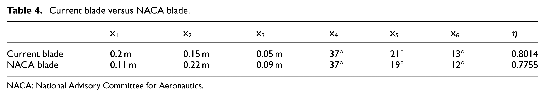
NACA: National Advisory Committee for Aeronautics.

In addition, CFD simulations are performed to analyze the performance of NACA blade and compare it with the performance of the current optimum design. Table 4 shows that our optimum blade has about 2.6% higher efficiency.

Off-design performance

The optimum blade has its peak efficiency near the design operating conditions (J = 0.6) and its performance decays progressively when operating at different flight conditions as shown in Figure 12. To maintain high efficiency during flight, aircrafts usually use variable pitch or constant speed propellers. This type of propellers allows changing the blade setting angle during flight so the propeller is always operating near the maximum obtainable efficiency for the current advance ratio. In other words, the propeller continuously adjusts its blade angle during flight to move on the maximum efficiency curve as shown in Figure 13. Blade angle is defined to be the pitch angle at 0.75R.

Figure 12.

Efficiency curve for the optimum blade at 17° blade angle.

Figure 13.

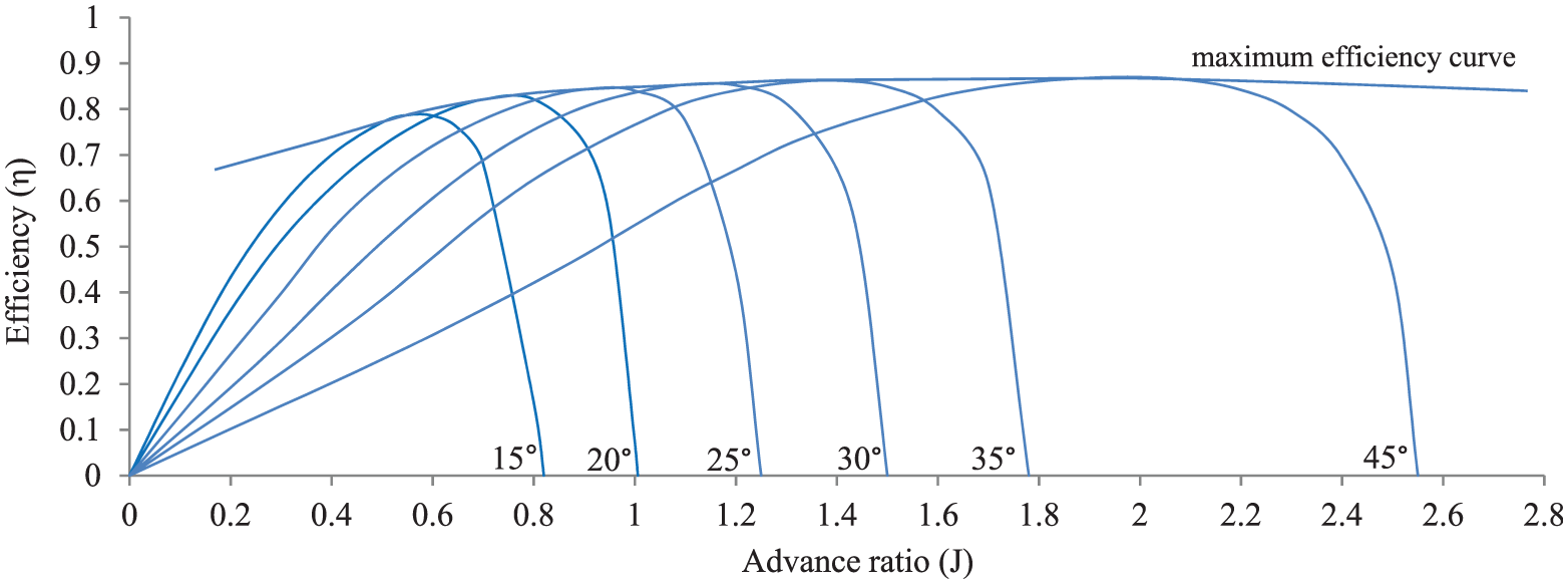
Efficiency curves for different blade angles.

At the design point (J = 0.6), the flow is laminar and attached to the blade surface with no separation on either the lower or upper airfoil surface. This is illustrated in Figure 14 by showing the velocity vectors and the turbulence kinetic energy near the airfoil. At a low advance ratio (J = 0.1), the flow faces the airfoil with a high positive angle of attack which forces the flow to separate at the upper surface of the airfoil as shown in Figure 15. On the contrary, at a high advance ratio (J = 0.85), the flow is oriented at a negative angle of attack which results in a flow separation on the airfoil lower surface as indicated in Figure 16. Flow separation results in an increase in pressure drag which increases the propeller torque and, hence, reduces the efficiency.

Figure 14.

Velocity vectors and turbulence kinetic energy at the design point (J = 0.6).

Figure 15.

Velocity vectors and turbulence kinetic energy at a low advance ratio off-design point (J = 0.1).

Figure 16.

Velocity vectors and turbulence kinetic energy at a high advance ratio off-design point (J = 0.85).

Kriging response surface optimization

ANSYS DesignXplorer integrated application is utilized as an alternative optimization tool to validate our results. The application uses a method based on DOEs and response surface optimization to find the optimum design point. Central composite design (CCD) and optimal space filling design (OSF) are used for sampling the design space. Kriging is used to generate a response surface for the efficiency from the sample points, and multi-objective genetic algorithm (MOGA) is then used to optimize the response surface. The process is repeated several times with different numbers of sample points. Table 5 summarizes the results.

Table 5.

Kriging response surface optimization.

DOE type	No. of sample points	Computational time (hours)	Optimum point $x_{f}^{*}$	Response $R_{f} (x_{f}^{*})$
CCD	45	89	[0.29 m, 0.15 m, 0.05 m, 31°, 21°, 14°]	0.7895
	56	111	[0.22 m, 0.17 m, 0.07 m, 35°, 21°, 9°]	0.7886
	65	129	[0.23 m, 0.15 m, 0.05 m, 37°, 20°, 12°]	0.7990
	70	138	[0.2 m, 0.15 m, 0.06 m, 35°, 25°, 10°]	0.7791
	75	146	[0.21 m, 0.15 m, 0.07 m, 31°, 25°, 10°]	0.7696
OSF	45	87	[0.21 m, 0.15 m, 0.05 m, 30°, 16°, 3°]	0.3442
	65	128	[0.29 m, 0.16 m, 0.05 m, 43°, 22°, 13°]	0.7935
	90	175	[0.21 m, 0.2 m, 0.07 m, 41°, 19°, 10°]	0.7857

DOE: design of experiment; CCD: Central composite design; OSF: optimal space filling design.

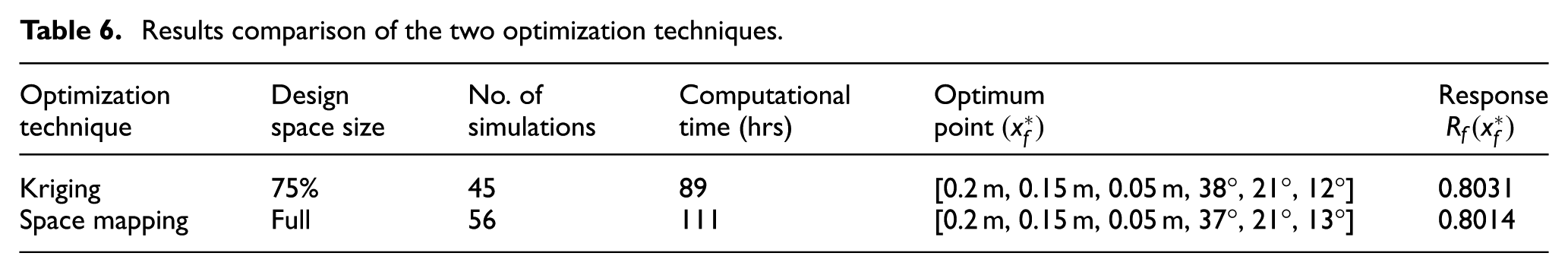
As the latter method failed to find the optimal point obtained by SM, the process is repeated after reducing the design space (to 75% of the original one) by reducing the design range of three parameters (pitch angles) by 50%. This time kriging response surface optimization obtained a very close optima to that obtained previously using SM (see Table 6). This emphasizes the validity of our results and proves that SM technique is more efficient for the full-size design space.

Table 6.

Results comparison of the two optimization techniques.

Optimizationtechnique	Designspace size	No. of simulations	Computationaltime (hrs)	Optimumpoint $(x_{f}^{*})$	Response $R_{f} (x_{f}^{*})$
Kriging	75%	45	89	[0.2 m, 0.15 m, 0.05 m, 38°, 21°, 12°]	0.8031
Space mapping	Full	56	111	[0.2 m, 0.15 m, 0.05 m, 37°, 21°, 13°]	0.8014

Case 2: five design cross-sections

In this case, five sections are considered; the main three sections of case 1 as well as two more sections in between. Thus, we have a total number of 10 design variables, $x \in R^{10}$ described as follows

x = [c_{1}, c_{2}, c_{3}, c_{4}, c_{5}, β_{1}, β_{2}, β_{3}, β_{4}, β_{5}]

(17)

where c_i, β_i, i = 1, 2,…, 5 are the chord length and pitch angle, respectively, at the five preassigned locations. This time, linear distributions of the chord length and pitch angle are assumed between each two successive sections as shown in Figure 17.

Figure 17.

Linear chord distribution between sections.

The lower-bound vector is set to be [0.2 m, 0.15 m, 0.15 m, 0.1 m, 0.05 m, 30°, 20°, 10°, 5°, 0°], whereas the upper-bound vector is taken [0.3 m, 0.3 m, 0.25 m, 0.2 m, 0.15 m, 50°, 40°, 30°, 25°, 20°]. The initial solution vector x_i is set to be [0.2 m, 0.25 m, 0.25 m, 0.2 m, 0.15 m, 60°, 45°, 30°, 20°, 15°]. From this initial solution, the algorithm obtained the coarse model optimum point x_c*. Then it is iterated and converged to the fine model optimum after five iterations with a total number of 66 fine model simulations. As the first case, the surrogate model response initially coincides with that of the coarse model and finally reaches, within acceptable error, the fine model response as shown in Figure 18. The convergence of the solution with iterations is presented in Table 7. A total improvement of 17% in the propeller efficiency is achieved.

Figure 18.

Variation of responses with iterations.

Table 7

Convergence of the solution (case 2).

Iteration	Solution vector $x^{(i)}$	$R_{f} (x^{(i)})$	$R_{s} (x^{(i)})$	$‖ R_{f} (x^{(i)}) - R_{s} (x^{(i)}) ‖^{2}$
0	$x_{i} = [0.2 m, 0.25 m, 0.25 m, 0.2 m, 0.15 m, 60^{°}, 45^{°}, 30^{°}, 20^{°}, 15^{°}]$	0.6865	0.7223	1.28E–03
0	$x_{c}^{*} = [0.2 m, 0.15 m, 0.15 m, 0.1 m, 0.05 m, 42^{°}, 27^{°}, 19^{°}, 15^{°}, 11^{°}]$	0.7968	0.8718	5.63E–03
1	$[0.2 m, 0.15 m, 0.15 m, 0.1 m, 0.05 m, 31^{°}, 31^{°}, 21^{°}, 18^{°}, 13^{°}]$	0.7984	0.811	1.59E–04
2	$[0.2 m, 0.15 m, 0.15 m, 0.1 m, 0.05 m, 50^{°}, 27^{°}, 23^{°}, 15^{°}, 12^{°}]$	0.7995	0.8175	3.24E–04
3	$[0.2 m, 0.15 m, 0.15 m, 0.1 m, 0.05 m, 50^{°}, 29^{°}, 19^{°}, 15^{°}, 15^{°}]$	0.8007	0.8153	2.13E–04
4	$[0.2 m, 0.15 m, 0.15 m, 0.1 m, 0.05 m, 37^{°}, 27^{°}, 21^{°}, 14^{°}, 14^{°}]$	0.7944	0.8124	3.24E–04
5	$[0.2 m, 0.18 m, 0.15 m, 0.1 m, 0.05 m, 37^{°}, 31^{°}, 21^{°}, 15^{°}, 15^{°}]$	0.8035	0.7997	1.44E–05

It is worth highlighting that this optimum point is very close to that obtained from case 1. The values of the six common parameters between the two cases are almost the same, and there are slight differences in the remaining four parameters as shown in Table 8. There is no significant improvement in the propeller efficiency between the two cases. This means that using only three sections to represent the blade shape is sufficient for the design optimization. The bold values in Table 8 are the design variables. Note that the values of the remaining four parameters in case 1 are obtained based on the values of the six design variables by assuming a second-order distribution along the blade radius, as mentioned before.

Table 8.

Results comparison between case 1 and case 2.

Case no.	Optimum point $(x_{f}^{*})$	Response $(R_{f} (x_{f}^{*}))$
1	[0.2 m, 0.18 m, 0.15 m, 0.11 m, 0.05 m, 37°, 28°, 21°, 16°, 13°]	0.8014
2	[0.2 m, 0.18 m, 0.15 m, 0.10 m, 0.05 m, 37°, 31°, 21°, 15°, 15°]	0.8035

Conclusion and future work

We combined the use of two common aerodynamic models in the field of propeller design to find the optimum propeller blade shape. BEM theory is used as a fast but coarse model, whereas a CFD model is used as a computationally expensive fine model to enhance the accuracy. The SM concept is exploited to replace the impractical direct optimization of the fine model by an iterative updating and re-optimization of a new surrogate model. Two cases are studied varying in the number of design parameters.

Furthermore, another technique is used to validate the results and compare the computational efficiency. It is based on sampling the design space using a DOE algorithm and generating a kriging response surface to be then optimized. This method is used for validating the results of only one of our two cases, since it would be very computationally expensive for the other. Although the two techniques obtained almost the same optimum point, the SM algorithm has the advantage of finding it with a smaller number of computationally expensive fine model evaluations.

This research has the potential for much future extension and development in some disciplines. First, regarding the optimization techniques, it may be useful to utilize more advanced techniques for the surrogate model optimization instead of using the MATLAB optimization toolbox. This might obtain more accurate results. Second, it is recommended to optimize the blade cross-sectional airfoil. This could be achieved by considering new design variables controlling the airfoil profile as well as those controlling the overall blade shape. In addition, for further refinement it is recommended to consider varying the airfoil shape along the blade radius instead of keeping it fixed.

Footnotes

Handling Editor: James Baldwin

Declaration of conflicting interests

The author(s) declared no potential conflicts of interest with respect to the research, authorship, and/or publication of this article.

Funding

The author(s) received no financial support for the research, authorship, and/or publication of this article.

ORCID iDs

Usama T Toman

Ahmed SA Mohamed

References

Mendoza

. Propeller design by numerical optimization. In: Business aircraft meeting, Wichita, KS, 29 March–1 April 1977, https://ntrs.nasa.gov/search.jsp?R=19770054220

Chang

Stefko

. Application of an optimization method to high performance propeller designs. In: 20th joint propulsion conference, Cincinnati, OH, 11–13 June 1984. Reston, VA: AIAA.

Rizk

Jou

. Propeller design by optimization. AIAA J 1986; 24: 1554–1556.

Cho

Lee

. Propeller blade shape optimization for efficiency improvement. Comput Fluids 1998; 27: 407–419.

Burger

Hartfield

Burkalter

. Propeller performance optimization using vortex lattice method and genetic algorithm. In: 44th AIAA aerospace sciences meeting and exhibit, Reno, NV, 9–12 January 2006, pp.12818–12831. Reston, VA: AIAA.

Gur

Rosen

. Optimization of propeller based propulsion system. J Aircraft 2009; 46: 95–106.

Zhao

Wang

et al . Aerodynamic propeller design using optimization method and genetic algorithm generation. In: Proceedings of 2010 Asia-Pacific international symposium on aerospace technology, Xi’an, China, 13–15 September 2010, pp.1019–1022. Northwestern Polytechnical University.

Sodja

Stadler

Kosel

. Computational fluid dynamics analysis of an optimized load-distribution propeller. J Aircraft 2012; 49: 955–961.

Droandi

Gibertini

. Aerodynamic shape optimisation of a proprotor and its validation by means of CFD and experiments. Aeronaut J 2015; 119: 1223–1251.

10.

Kwon

H-I

Choi

et al . Design of efficient propellers using variable-fidelity aerodynamic analysis and multilevel optimization. J Propul Power 2015; 31: 1057–1072.

11.

Morgado

Abdollahzadeh

Silvestre

MAR

et al . High altitude propeller design and analysis. Aerosp Sci Technol 2015; 45: 398–407.

12.

Koziel

Yang

X-S

. Surrogate-based methods. In: Koziel

Yang

X-S

(eds) Computational optimization, methods and algorithms. Berlin: Springer-Verlag, 2011, pp.34–59.

13.

Wang

Wei

et al . Application of DOE in optimization of geometric parameters of the propeller. Ship Build China 2015; 56: 109–118.

14.

Song

Keane

. Surrogate-based aerodynamic shape optimization of a civil aircraft engine nacelle. AIAA J 2007; 45: 2565–2574.

15.

Samad

Kim

K-Y

Goel

et al . Multiple surrogate modeling for axial compressor blade shape optimization. J Propul Power 2008; 24: 302–310.

16.

Mukesh

Lingadurai

Selvakumar

. Kriging methodology for surrogate-based airfoil shape optimization. Arab J Sci Eng 2014; 39: 7363–7373.

17.

Leifsson

Koziel

Tesfahunegn

. Multiobjective aerodynamic optimization by variable-fidelity models and response surface surrogates. AIAA J 2016; 54: 531–541.

18.

Vesting

Bensow

. On surrogate methods in propeller optimisation. Ocean Eng 2014; 88: 214–227.

19.

Marinus

Roger

Van Den Braembussche

. Aeroacoustic and aerodynamic optimization of aircraft propeller blades. In: 16th AIAA/CEAS aeroacoustics conference, Stockholm, 7–9 June 2010. Reston, VA: AIAA.

20.

Carroll

Marcum

. Local adaption capabilities of momentum source surrogate propeller models for propeller-aircraft coupled simulations. Eng Lett 2013; 21: 247–255.

21.

Koziel

Leifsson

. Surrogate-based aerodynamic shape optimization by variable-resolution models. AIAA J 2013; 51: 94–106.

22.

Koziel

Tesfahunegn

Leifsson

. Expedited constrained multi-objective aerodynamic shape optimization by means of physics-based surrogates. Appl Math Model 2016; 40: 7204–7215.

23.

Bandler

Biernacki

Chen

et al . Space mapping technique for electromagnetic optimization. IEEE T Microw Theory 1994; 42: 2536–2544.

24.

Bandler

Cheng

Dakroury

et al . Space mapping: the state of the art. IEEE T Microw Theory 2004; 52: 337–361.

25.

Koziel

Leifsson

. Knowledge-based airfoil shape optimization using space mapping. In: 30th AIAA applied aerodynamics conference, New Orleans, LA, 25–28 June 2012, pp.1390–1399. Reston, VA: AIAA.

26.

Tesfahunegn

Koziel

Leifsson

et al . Surrogate-based airfoil design with space mapping and adjoint sensitivity. Procedia Comput Sci 2015; 51: 795–804.

27.

Leifsson

Tesfahunegn

Koziel

Tesfahunegn

et al . Aerodynamic design optimization: physics-based surrogate approaches for airfoil and wing design. In: 52nd AIAA aerospace sciences meeting—AIAA science and technology forum and exposition, National Harbor, MD, 13–17 January 2014. Reston, VA: AIAA.

28.

Robinson

Eldred

Willcox

et al . Surrogate-based optimization using multifidelity models with variable parameterization and corrected space mapping. AIAA J 2008; 46: 2814–2822.

29.

Koziel

Leifsson

. Wing shape optimization using local response surface approximations, space mapping and physics-based surrogates. In: 52nd AIAA aerospace sciences meeting—AIAA science and technology forum and exposition, National Harbor, MD, 13–17 January 2014. Reston, VA: AIAA.

30.

Silvestre

MAR

Morgado

Páscoa

. JBLADE: a propeller design and analysis code. In: 2013 international powered lift conference, Los Angeles, CA, 12–14 August 2013. Reston, VA: AIAA.

31.

Chen

Pan

. Efficient lifting line method for computing performance of propeller. Hangkong Dongli Xuebao/J Aerosp Power 1991; 6: 295–299.

32.

Hess

Valarezo

. Calculation of steady flow about propellers using a surface panel method. J Propul Power 1985; 1: 470–476.

33.

Chang

Sullivan

. Optimization of propeller blade twist by an analytical method. AIAA J 1984; 22: 252–255.

34.

Bandler

Biernacki

Chen

. Fully automated space mapping optimization of 3D structures. In: IEEE MTT-S international microwave symposium digest, San Francisco, CA, 17–21 June 1996, pp.753–756. New York: IEEE.

35.

Bandler

Biernacki

Chen

et al . Space mapping optimization of waveguide filters using finite element and mode-matching electromagnetic simulators. Int J RF Microw C E 1999; 9: 54–70.

36.

Bandler

Biernacki

Chen

et al . Design optimization of interdigital filters using aggressive space mapping and decomposition. IEEE T Microw Theory 1997; 45: 761–769.

37.

Bakr

Bandler

Georgieva

. An aggressive approach to parameter extraction. IEEE T Microw Theory 1999; 47: 2428–2439.

38.

Bandler

Mohamed

Bakr

et al . EM-based optimization exploiting partial space mapping and exact sensitivities. IEEE T Microw Theory 2002; 50: 2741–2750.

39.

Koziel

Bandler

Madsen

. Space mapping optimization algorithms for engineering design. In: IEEE MTT-S international microwave symposium digest, San Francisco, CA, 11–16 June 2006, pp.1601–1604. New York: IEEE.

40.

Koziel

Bandler

Madsen

. A space—mapping framework for engineering optimization—theory and implementation. IEEE T Microw Theory 2006; 54: 3721–3730.

41.

ANSYS Fluent 14.0 user’s guide. 2011.

42.

Morgado

Silvestre

MÂR

Páscoa

. Validation of new formulations for propeller analysis. J Propul Power 2015; 31: 467–477.

43.

Biermann

Hartman Edwin

. Tests of two full-scale propeller with different pitch distributions, at blade angles up to 60. Technical report no. 658, 1938, https://ntrs.nasa.gov/search.jsp?R=19930091733

Blade shape optimization of an aircraft propeller using space mapping surrogates

Abstract

Keywords

Introduction

Design problem formulation

Design variables and preassigned parameters

Propeller aerodynamic efficiency

Design constraints

Aerodynamic models

BEM theory

CFD

SM-based optimization

Implementations

Coarse model

Fine model

Mesh-sensitivity analysis

Validation of the numerical solution

Comparing the coarse and fine model responses

SM algorithm

Sensitivity analysis

Results and discussions

Case 1: three design cross-sections

Comparing the current optimal design with a NACA blade design

Off-design performance

Kriging response surface optimization

Case 2: five design cross-sections

Conclusion and future work

Footnotes

Declaration of conflicting interests

Funding

ORCID iDs

References