Sage Journals: Discover world-class research

Abstract

A promoter is a brief stretch of DNA (100–1,000 bp) where RNA polymerase starts to transcribe a gene. A DNA (Deoxyribonucleic Acid) base pair is a fundamental unit of DNA structure and represents the pairing of two complementary nucleotide bases within the DNA double helix. The four DNA nucleotide bases are adenine (A), thymine (T), cytosine (C), and guanine (G). DNA base pairs are the building blocks of the DNA molecule, and their complementary pairing is central to the storage and transmission of genetic information in all living organisms. Normally, a promoter is found at the 5 ${}^{\prime}$ end of the transcription initiation site or immediately upstream. Numerous human disorders, particularly diabetes, cancer, and Huntington’s disease, have been shown to have DNA promoter as their root cause. The scientific community has long been interested in learning crucial information about protein-coding genes. Finding the promoters is therefore the first step in finding genes in DNA sequences. The scientific world has always been attracted by the effort to glean crucial knowledge about protein-coding genes. Consequently, identifying promoters has emerged as an intriguing challenge that has caught the interest of numerous researchers in the field of bioinformatics. We proposed Gaussian Decision Boundary Estimation in machine learning models to detect transcription start sites (promoters) in the DNA sequences of a common bacteria, Escherichia coli. The best features are identified through a score-based function to select relevant nucleotides that are directly responsible for promoter recognition, in order maximise the models’ performance. The Gaussian Decision Boundary Estimation based support-vector-machine model is trained with these features and finds the best hyperplane that separates the data into different classes. Throughout this study, promoter regions could be identified with high accuracy 99.9% which is better compared to other state of art algorithms. The comparison of machine learning classification models is another major emphasis of this paper in order to identify the model that most accurately predicts DNA sequence promoters. It provides analysis for further biological research as well as precision medicine.

Keywords

Promoter DNA Bioinformatics machine learning gaussian decision boundary estimation

1. Introduction

The promoter, a section of DNA, is where RNA polymerase binds to start a gene’s transcription process. According to Lin et al. (2018), promoter sequences are commonly found right before or at the 5 ${}^{\prime}$ end of the transcription initiation site. RNA polymerase and the required transcription factors are able to recognise both promoters and transcription initiation sites. Promoter sequences identify the sense strand of DNA that will be transcribed and show the direction of the transcription. Figure 1 depicts the two phases of the transcription process: activating and deactivating genes. Promoters use the data RNA polymerase provides them in these two stages to predict how lactase will be produced. Promoters can range in length from 100 to 1,000 base pairs.

Deoxyribonucleic acid, sometimes known as DNA, is the special genetic code that is responsible for the coordination and functioning of all living beings. DNA consists a double-helix polymer, a spiral consisting of two DNA strands wound around each other [1]. The DNA of almost every cell in a person’s body is identical. The four chemical bases adenine (A), guanine (G), cytosine (C), and thymine (T) make up the DNA code. Each base also has a sugar and phosphate molecule connected to it; this grouping of bases, sugars, and phosphates is known as a nucleotide. The genome of the organism is made up of the set of chromosomes that make up the DNA within each cell. The majority of the DNA in eukaryotes that is not expressed in an amino acid chain of a protein is referred to as “junk DNA”. It is known that only 1.5% of human genome is to be protein-coding [2]. Only one copy of the DNA from the parent organism is present in each cell, and it is located in the nucleus. Therefore, the cell creates a copy of that specific code segment called ribonucleic acid (RNA) inside its nucleus in order to use that particular component of the DNA code.

The promoter region of the DNA plays a key regulatory role in gene expression. A promoter is a section of DNA that designates a gene’s transcriptional start site. An enzyme known as RNA polymerase II binds to a promoter to carry out transcription shown in Fig. 1, in which DNA is converted into RNA, which is then spliced into an mRNA, which is then translated into a protein.

Promoters differ at their consensus sequence according on the RNA polymerase’s factor used, which provides DNA recognition specificity [11, 12]. The plethora of experimentally known promoter sequences for several growth factors in various organisms has made it possible to apply prediction approaches based on the construction of Position-Weight Matrices (PWM), which uncover conserved canonical motifs. The high frequency of false positive predictions with partial coverage, however, limits the effectiveness of these approaches [13, 15].

The present study used a dataset with 106 DNA sequences, each with 57 consecutive nucleotides, from the UCI Machine Learning Repository. In this study, the problem of identifying transcription sites, which entails identifying promoter sequences in short DNA sequences of Escherichia coli bacterium, is resolved. The precise prediction of promoter sites is essential for comprehending gene expression, deciphering patterns, and constructing genetic regulatory networks because promoters are now so crucial for transcription.

Figure 1.

Transcription process [8].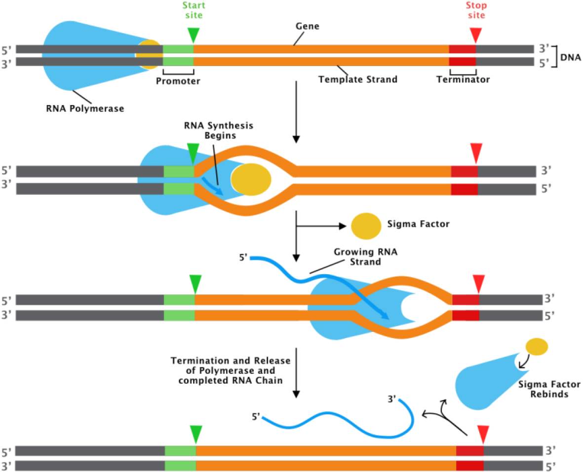

In addition to this, promoter prediction is a crucial step in the genome annotation process because it allows for the identification of novel genes, particularly those linked to non-coding RNA, which are frequently overlooked by gene prediction algorithms. Although numerous intricate feature extraction strategies and numerous classifiers have been put out so far for promoter recognition, the issue is still unresolved [17]. A significant barrier to bioinformatics’ genome-wide investigation of gene regulation is the inability to predict promoters [18].

The database of E. coli experimentally determined promoters has been significantly increased by our extensive promoter identification work, which will encourage experimental biologists to investigate the gene expression mechanisms underlying some of these genes, particularly for those without a known biological function.

Here, the Gaussian Decision Boundary Estimation in machine learning models is proposed to classify the promoters based on the DNA sequence.In order to maximise the performance of the models, the best features are determined using a score-based algorithm to choose pertinent nucleotides that are directly responsible for promoter recognition. With the help of these features, the support-vector-machine model, which is based on Gaussian Decision Boundary Estimation, is trained to identify the optimal hyperplane for classifying the data.

2. Related work

Numerous attempts have been made to recognise promoters using computational methods. Basic Local Alignment Search Tool (BLAST) is a search technique that Altschul et al. [3] proposed as a method for determining the similarity between two genetic sequences. Towel et al. [4] proposed the KBANN (Knowledge-Based Artificial Neural Networks)hybrid learning system. This system blends explanation-based learning with empirical learning for promoter prediction. Using multilayer perceptron neural networks, Weinert et al. [5] describe a quick and effective biomolecular classification methodology that is used to categorise proteins and infer their functions by comparing their structural similarity. Gordon et al. [22] developed an approach for prediction of promoters and Transcription Start Sites in E. coli, based on an ensemble of Support Vector Machines and this classifier is then combined with Position Weight Matrices. It is concluded that an ensemble-SVM with mismatch string kernels may be able to identify and take use of a variety of regulatory motifs for improved TSS/promoter detection.

To predict promoter sequences in the DNA of E. coli bacteria, Tavares et al. [6] examined the efficacy of various machine learning algorithms. In this comparative investigation, results from probabilistic methods like the Hidden Markov Model (HMM) and Bayesian methods are more precise. ANN shave has proven acceptable profound results, but the high false positive rate [20, 21] has affected the specificity. Kemal Polat et al. [10] proposed a novel method based on feature selection (FS) and Artificial Immune Recognition System (AIRS) with Fuzzy resource allocation mechanism (Fuzzy-AIRS) for identifying promoters in strings that represent nucleotides.

Karlı G et al. [9] developed a new method known as IREM (Inductive Rule Extraction Method) for solving the problem. Attribute-value pairs with higher information value is determined by IREM. It uses its own “cost function” to determine how much information each pair in the set is worth. It discussed the notion that a lower cost is a sign of a higher information value. Attribute-values with higher values are given a higher priority while creating the rule base of the forecasting system.

Anveshrithaa et al. [7] observed that promoters in DNA sequences are best classified using neural networks trained with back-propagation. The back-propagation optimisation and grid search hyperparameter tuning are credited with the excellent accuracy. It is discovered that additional models, such as the ensemble learning technique Bootstrap Aggregation and the Support Vector Machine with linear kernel, are as good in categorising DNA sequences. The comparison of the various methods applied to the task of identifying promoters in DNA sequence is shown in Table 1.

Khan z, Rajdeep et al. [8] claimed an improved accuracy by selective choice of hyperparameters for Multilayer Perceptron (MLP) Neural Network in Promoter Identification. Numerous alternative computational techniques have also been put forth. However, the vast majority of these methods do not result in promoter recognition accuracy rates that are satisfactory.

The Inductive Rule Extraction approach is introduced by Karl et al. [9], while the Fuzzy-AIRS classifier and feature selection are used by Polat et al. [10] to identify the DNA sequence’s promoters. For the classification of the promoters from the DNA sequence, Towel et al. [4] and Weinert et al. [5] implement Knowledge-Based Artificial Neural Networks and Multilayer Perceptron Neural Networks, respectively.

Table 1
Comparison of proposed model with other state of art algorithms

Author	Methodology	Accuracy	F1-Score	Precision	Recall
Tavares et al. [6]	MLP	0.9340	0.93	0.94	0.92
Anveshrithaa et al. [7]	ANN with backpropagation	0.9687	0.97	0.97	0.97
Khan z, Rajdeep et al. [8]	MLP	0.96	0.96	0.95	0.97
Proposed model	Gaussian decision boundary estimation	99.9	0.999	1.0	0.999

3. Methodology

An overall flowchart of the strategy used is shown in Fig. 2, which operates using a specially created pipeline. In the subsections that follow, each experimental step of this suggested pipeline will be discussed in turn.

The main contribution of the work is listed here,

•
The dataset required for identification of promoters in DNA sequences is collected and analysed from the UCI Repository. It contained a set of 106 DNA sequences and their corresponding classes (Promoter or Non-Promoter).
•
The DNA sequences are split into 57 individual nucleotides each and are converted to numerical data through one hot encoding by replacing each categorical column in the DataFrame with a set of binary columns which is followed by transformation of the dataset into polynomial feature matrix of degree 2.
•
The ANOVA F-value for each feature in the feature matrix is computed and the top 1000 features are extracted for training and testing.
•
The width of the gaussian function is determined by computing the gamma ( $\gamma$ ) value for the input data and the original feature space is transformed into a higher-dimensional feature space.
•
The optimal hyperplane that maximizes the margin between the classes in the transformed feature space are found using the pairwise similarities.

Figure 2.
Proposed architecture.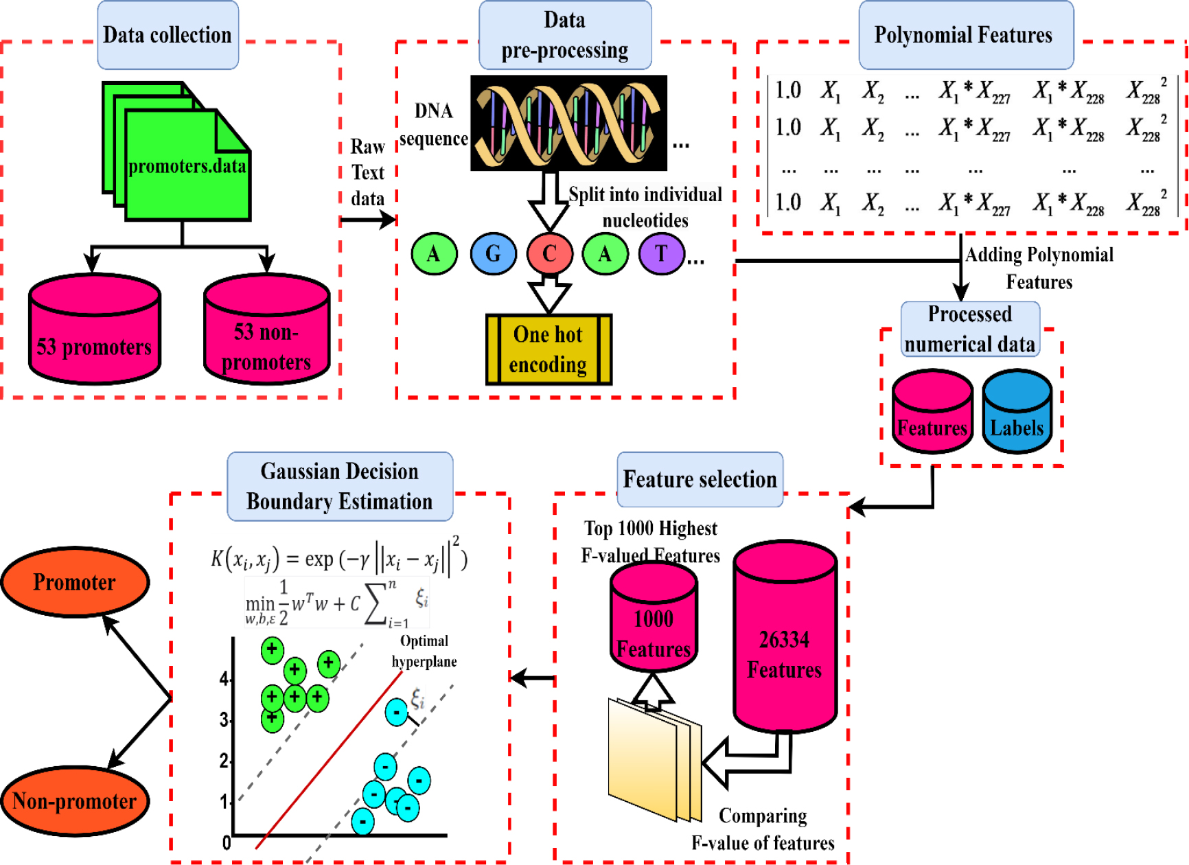

3.1 Data collection

One of the most crucial phases in solving a bioinformatics issue is gathering a high-quality dataset. To unbiasedly compare the performance of our model to other ones already in use, we used the benchmark dataset from the UCI repository in this study.

The dataset for the proposed study is found in the UCI Machine Learning Repository (https://archive.ics.uci.edu/ml/machine-learning-databases/molecular-biology/promoter-gene-sequences/promoters.data). The datasetencompasses 106 DNA sequences. Each DNA sequence comprises of 57 consecutive nucleotides. The dataset contains 53 Promoter sequences and 53 Non promoter sequences. DNA nucleotides can be grouped into a hierarchy, as shown in Fig. 3.

Figure 3.

Hierarchy of the DNA nucleotides.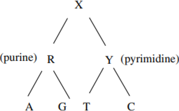

DNA nucleotides can be categorized into two distinct groups: purines, which encompass adenine and guanine, and pyrimidines, which encompass cytosine and thymine in the context of DNA, and uracil when considering RNA. This categorization is predicated upon the structural characteristics of their respective nitrogenous bases.

Purines: Purines constitute a class of nitrogenous bases present within the DNA molecule, characterized by their dual-ring structure. Within DNA, there exist two primary purine bases:

Adenine (A): Adenine represents one of the quartet of nitrogenous bases forming the DNA structure. It engages in the formation of hydrogen bonds with thymine (T) in complementary base pairs within the DNA double helix. In the context of RNA, adenine instead pairs with uracil (U).

Guanine (G): Guanine, another purine base present in DNA, pairs with cytosine (C) through the mediation of hydrogen bonds. Notably, guanine also maintains its pairing with cytosine in RNA structures.

ii)

Pyrimidines: Pyrimidines, the other class of nitrogenous bases within DNA, possess a singular-ring structure. Within DNA, three pyrimidine bases are identified:

Cytosine (C): Cytosine, a pyrimidine base, pairs with guanine in DNA through hydrogen bonding interactions. Remarkably, cytosine also exhibits this pairing behaviour with guanine in the realm of RNA.

Thymine (T): Thymine, as another pyrimidine base in DNA, forms specific hydrogen bond interactions with adenine. However, it is essential to note that in RNA, thymine is replaced by uracil (U), which similarly pairs with adenine.

Uracil (U): Uracil, exclusive to RNA, represents a pyrimidine base. In RNA molecules, uracil engages in hydrogen bond-based pairing with adenine, mirroring the role of thymine in DNA.

The DNA sequences in the dataset are divided into two classifications, “ $+/-$ ”, with “ $+$ ” denoting a promoter. The sequence of the remaining 57 fields is from position $-$ 50 (p-50) to position $+$ 7 (p. 7). Adenine, Thymine, Guanine, and Cytosine – abbreviated as $a$ , $g$ , $t$ , and $c$ – are each filled in one of these fields [19]. 57 consecutive DNA nucleotides make up the input characteristics.

The dataset contains a balanced number of samples for each class. A balanced dataset, where each class has an equal number of samples, helps prevent class imbalance issues. Class imbalance can bias the model towards the majority class, making it less sensitive to the minority class. Also, a balanced dataset allows for a more accurate assessment of the model’s classification performance.

3.2 Preprocessing

The UCI Repository’s data is not in a format that may be used. Prior to training various machine learning models, datasets are pre-processed. Individual nucleotides are separated into the DNA sequences. The numerical data is to be converted from the textual data corresponding to the different nucleotides. One-hot encoding is accomplished for the conversion. One-hot encoding is a technique used to convert categorical data into a binary vector representation [24]. One-hot encoding preserves all the information in the categorical variable. One-hot encoding was used rather than other methods as many encoding methods (e.g., label encoding) assign integer values to categories, which could introduce a magnitude bias. Models might misinterpret the magnitude of these values as meaningful information. One-hot encoding eliminates this issue by using binary values. One-hot encoding also prevents biasing the model towards the category with higher integer values, ensuring that all categories have equal weight. A binary column isgenerated for each categorical column (A, C, G, T and $+$ , $-$ ) in the DataFrame. If a nucleotide or its class matched the value of the binary column, the column is filled with 1, else it is filled with 0. This process resulted in 228 input features after encoding, as each DNA sequence comprised 57 nucleotides belonging to one of the four categories (A, C, G, T). The input features are then separated from their respective labels, facilitating the subsequent machine learning model training.

Polynomial features are generated from the set of encoded features. The encoded input feature matrix $X$ is transformed into a new matrix $X_{\textit{poly}}$ by inclusion of new columns representing the polynomial combinations of the original features. Non-linear relationships between the original featurescan be capturedby including polynomial features, which potentially improves the performance of machine learning models that rely on these features. Considering nonlinear features adds complexity to the model [23]. All conceivable arrangements of the input features up to the second degree are taken into consideration when creating polynomial features. As the degree of polynomial features generated increases, the model becomes more complex and can start fitting the noise in the training data, leading to poor generalization to new, unseen data. Increasing the polynomial degree also results in higher-dimensional feature spaces. In such spaces, the number of dimensions grows rapidly, and data points become sparser. This can lead to difficulties in separating classes effectively and make the Gaussian Decision Boundary Estimator’s optimization problem more challenging. As the polynomial degree increases, the decision boundary becomes more flexible and intricate. This might lead to high variance in the predictions, causing the model to be sensitive to small fluctuations in the input data. Thus, The degree of polynomial features generated is limited to 2. The multinomial coefficient, also referred to as the binomial coefficient, is used to generate polynomial combinations. The number of combinations for the feature matrix, with $n\_\textit{features}$ for a degree of 2 is given by:

$\displaystyle C=\frac{\left({n_{\textit{features}}+2}\right)!}{\left({2!}% \right)\ast\left({n_{\textit{features}}}\right)!}$

A new feature matrix is created from the original feature matrixand the dataset is transformed into polynomial features. In accordance with the calculation above, each of the 106 DNA sequences will be equipped with 26335 features in the updated feature matrix $X\_\textit{poly}$ . The matrix had a shape of (106, 26395) after he transformation. Each row represented a sample and each column represented a specific feature (original feature or pairwise product) obtained from the polynomial transformation. The polynomial transformation can be represented by the equation:

$\displaystyle\textit{Poly}_{\textit{features}}=[x_{1},x_{1}^{2},x_{1}x_{2},x_{% 1}x_{3},\ldots,x_{M},x_{M}^{2},x_{2}^{2},x_{2}x_{3},\ldots]$

Where, $M$ denotes the number of features, i.e., 228. This equation represents the polynomial features for a single sample. It includes the original features themselves $\left({x1,x2,\ldots,xM}\right)$ and their pairwise products up to degree 2. The notation $x_{i}^{2}$ represents the square of the $i^{\textit{th}}$ feature, and $x_{i}x_{j}$ represents the product of the $i^{\textit{th}}$ and $j^{\textit{th}}$ features. The ellipsis (…) indicate that the pattern is consistent for all pairwise products between the features. The transformed dataset is split into training and testing data (30% test data). Algorithm 1 shows the feature extraction method used in the proposed method.

Algorithm 1: Feature extraction
Input: Feature matrix X with shape $\left({n\_\textit{samples},n\_\textit{features}}\right),$ where $n\_\textit{samples}$ denotes the number of samples and $n\_\textit{features}$ denotes the number of original features.
Output: Transformed matrix $X\_\textit{poly}$ , containing the original features along with their polynomial combinations
1. Initialize an empty matrix $X\_\textit{poly}$ with shape $\left({n\_\textit{samples},1}\right)$ , which stores the polynomial features.
2. For each sample in $X$ :
a. Create an empty row vector $\textit{poly}\_\textit{row}$ to store the polynomial combinations for that sample.
b. For each feature in the sample: i. Compute the polynomial combinations of the feature with itself (degree 1) and add them to $\textit{poly}\_\textit{row}$ . ii. For each subsequent degree from 2 up to the specified degree: $-$ Compute the polynomial combinations of the feature with all other features of equal or lower degree. $-$ Add these combinations to $\textit{poly}\_\textit{row}$ . c. Append $\textit{poly}\_\textit{row}$ to $X\_\textit{poly}$ .
3. return $X\_\textit{poly}$

3.3 Feature selection using $f\_\textit{classif}$ score function

Feature extraction is a pivotal step in bioinformatics problem-solving, wherein primary features play a crucial role in distinguishing DNA sequences. The abundance of attributes and occurrences in raw datasets often poses significant challenges for data mining systems. A proven remedy to address this issue is feature selection, which aims to identify a compact subset of relevant features while retaining the original purpose through justifiable criteria. By eliminating irrelevant and redundant features, this process results in a simplified dataset, yielding more concise and comprehensible outcomes. The top 1000 features from the feature matrix are selected based on the ‘f_classif’ scoring function and the training data is fitted. The SelectKBest function in the scikit-learn package is used to accomplish this [16].

The f_classif function computes the ANOVA (analysis of variance) F-value between each feature and the target variable. ANOVAor Analysis of Variance, is a statistical technique used to compare means of two or more groups to determine if there are significant differences between them. It helps in understanding whether a categorical factor has a statistically significant impact on a continuous outcome variable. The ANOVA F-value is a statistical measure used to compare the means of two or more groups. It assesses whether the differences in means among these groups are likely due to real differences in the population or random variation. A high F-value, along with a small p-value, suggests significant differences among group means, indicating that the factor being tested has a statistically significant effect on the dependent variable. The higher the F-value, the more likely the feature is to be relevant for classification. A new feature matrix is created containing the top 1000 features determined by the F-value. The proposed method utilizes ANOVA as a set of parametric statistical models and associated estimation techniques to assess whether the means of multiple data samples originate from the same distribution. Each feature is subjected to a univariate statistical test, as it is compared to the target feature, facilitating the identification of statistically significant associations [25].

The F-valueis computed as follows:

$\displaystyle\textit{variance}\_\textit{between}\_\textit{groups }=\frac{% \mathop{\sum}\nolimits_{i=1}^{j}j_{i}\left(\bar{K}_{i}-\bar{K}\right)^{2}}{(S-% 1)}$ $\displaystyle\textit{variance}\_\textit{within}\_\textit{groups}=\frac{\mathop% {\sum}\nolimits_{i=1}^{S}\mathop{\sum}\nolimits_{p=1}^{j_{i}}\left({K_{ip}-% \bar{K_{i}}}\right)^{2}}{\left({N-S}\right)}$ $\displaystyle F\_\textit{value}=\frac{\textit{variance}\_\textit{between}\_% \textit{groups}}{\textit{variance}\_\textit{within}\_\textit{groups}}$

Where,

$N$ – Overall sample size.

$S$ – Number of groups.

$j_{i}$ – Number of observations in the $i^{\text{th}}$ group.

$\bar{K_{i}}-i^{\text{th}}$ group sample mean.

$K$ – Overall mean of the data.

$K_{ip}-p^{\text{th}}$ observation in the $i^{\text{th}}$ out of S groups.

$\textit{Between}\_\textit{group variability}$ – variance of the means of each class.

$\textit{Within}\_\textit{group variability}$ – variance of the samples within each class.

A higher between-group variance signifies a more pronounced distinction between the classes, implying increased relevance of the feature for classification purposes. To identify the most pertinent attributes for classification, the selection of the top 1000 features based on their F-valuesis employed, favouring those with the greatest F-values.

3.4 Gaussian decision boundary estimation

Support Vector Machines are a class of supervised machine learning models employed for tasks involving classification and regression. These models aim to construct a hyperplane (as illustrated in Fig. 3) within a high-dimensional feature space, with the primary objective of maximizing the separation between the two classes denoted by “ $+$ ” and “ $-$ ”. By employing SVMs, the issue of overfitting can be effectively managed [26]. Following the transformation of data into the new dimension, the SVM algorithm searches for a linear hyperplane that effectively separates the data points in this augmented feature space [27].

The Radial Basis Function (RBF) kernel, also known as the Gaussian kernel, stands out as a prominent choice for evaluating the similarity between two samples. The RBF kernel is defined as:

$\displaystyle K\left({x_{i},x_{j}}\right)=\mbox{exp}\left({-\gamma\left|{\left% |{x_{i}-x_{j}}\right|}\right|^{2}}\right)$

Where, $\gamma$ is a hyperparameter that controls the width of the kernel and $\left|{\left|{x_{i}-x_{j}}\right|}\right|^{2}$ is the squared Euclidean distance between the two input vectors $x_{i}$ and $x_{j}$ . In our model, the value of gamma is set to ‘scale’ which is computed as:

$\displaystyle\gamma=\frac{1}{\textit{Number of features}\ast\textit{Variance % of input data}}$

The number of features taken is 1000, thus

$\displaystyle\gamma=\frac{1}{1000\ast\textit{Variance of input data}}$

The input data are transformed by the RBF kernel into a higher dimensional space where they are more linearly separated. The optimization problem can be formulated as:

$\displaystyle\mathop{\min}\limits_{w,b,\varepsilon}\frac{1}{2}w^{T}w+C\mathop{% \sum}\limits_{i=1}^{n}\xi_{i}$

subject to:

$\displaystyle y_{i}\left({w^{T}\varphi\left({x_{i}}\right)+b}\right)\geqslant 1% -\xi_{i}$

$\displaystyle\xi_{i}\geqslant 0$

Where,

$w$ – weight vector.

$b$ – bias term.

$\xi_{i}$ – slack variables that allow for some misclassification.

$C$ – hyperparameter that controls the trade-off between maximizing the margin and minimizing the classification error.

$\varphi(x_{i})$ – feature vector obtained by applying the RBF kernel to the input vector $x_{i}$ .

Figure 4.

SVM Hyperplane.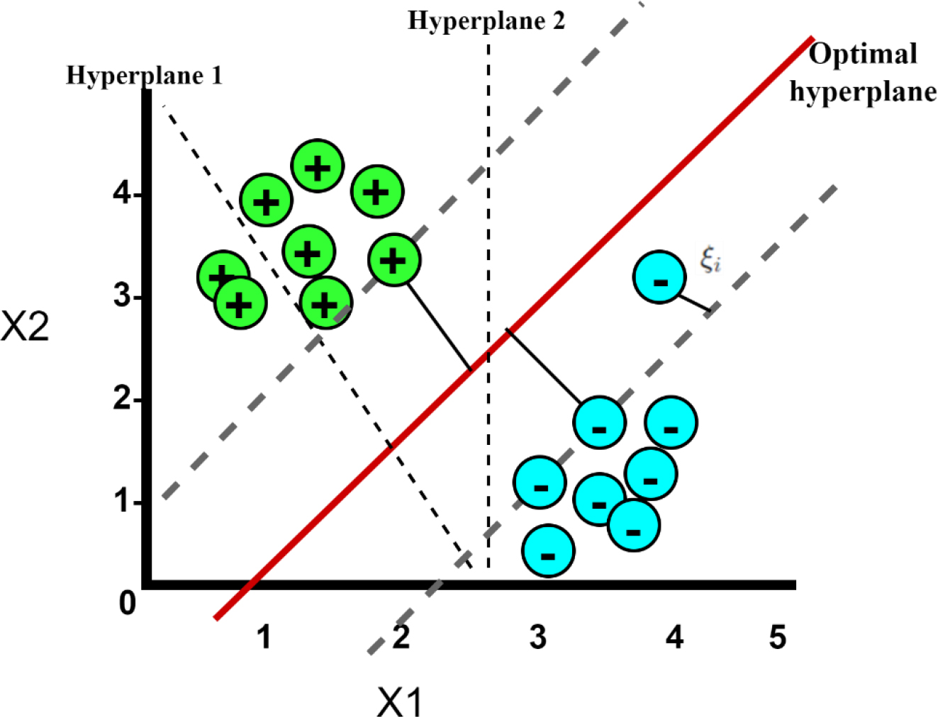

The slack variable represents the amount by which data points are allowed to violate the margin and the classification boundary. They quantify the degree of misclassification for each data point and represents how far a data point is from being correctly classified. The slack variable transforms the hard constraints of perfectly classifying all data points, which might not be feasible, into soft constraints, making the model more flexible and adaptable to complex datasets. It plays a significant role in finding a balance between maximizing the margin and minimizing classification errors, thereby making the model effective for a wide range of classification tasks.

The decision function has the following equation after the Lagrange duality approach yields the dual version of this optimisation problem:

$\displaystyle f\left(x\right)=\mathop{\sum}\limits_{i=1}^{n}\alpha_{i}y_{i}K% \left({x_{i},x}\right)+b$

Where,

$\alpha_{i}$ – Lagrange multipliers.

${K}\left({{x}_{i},{x}}\right)$ – RBF kernel evaluated at the support vectors and the test point $x$ .

The Gaussian Decision Boundary estimator is trained on the transformed and selected training data. For every pair of samples $(x_{i},x_{j})$ , the similarity is computed by evaluating the exponential of the Euclidean distance between the samples. This distance is scaled by the gamma parameter, resulting in the transformation of the original feature space into a higher-dimensional space. Consequently, samples that are closely situated in the original space exhibit increased similarity in the transformed space. The pairwise similarities serve as the foundation for identification of the optimal hyperplane that maximizes the margin between the classes within the transformed feature space. Subsequently, the model parameters, encompassing support vectors, coefficients, and bias, are optimized to ascertain the most effective hyperplane for class separation within the training data. Ultimately, the similarity between each support vector and the new sample is computed and combined with the learned model parameters to facilitate prediction.

Algorithm 2: Input: Raw data-DNA sequences. Output: Promoter/Non-promoter

Split the DNA sequences into individual nucleotides. 2.

Replace each categorical column in the split data with a set of binary columns, where each column corresponds to a unique value in the original column

Transform the dataset into polynomial feature matrix of degree 2

Split the data into training and testing datasets with a test size $=$ 0.3

Compute the ANOVA F-value for each feature in the feature matrix with respect to the target variable array.

Rank the features in descending order based on their F-values

Select the top 1000 features based on their rankings

Transform the feature matrix, retain only the selected top K features and discard the remaining features.

Compute the gamma ( $\gamma)$ value, which determines the width of the Gaussian function

10.

For each pair of samples (x ${}_{i}$ , x ${}_{j})$ , compute the similarity as the exponential of the Euclidean distance between the samples, scaled by the gamma parameter

11.

Transform the original feature space into a higher-dimensional feature space, where samples that are closer in the original space have a higher similarity in the transformed space

12.

Use the pairwise similarities to find the optimal hyperplane that maximizes the margin between the classes in the transformed feature space

13.

Optimize the model parameters (including support vectors, coefficients, and bias) to find the hyperplane that best separates the classes, in the training data.

14.

Compute the similarity between each support vector and the new sample, then combine these similarities with the learned model parameters and predict whether the given sequence is a promoter or non-promoter.

Figure 5.

Frequency of classes (1-promoter, 0- non-promoter).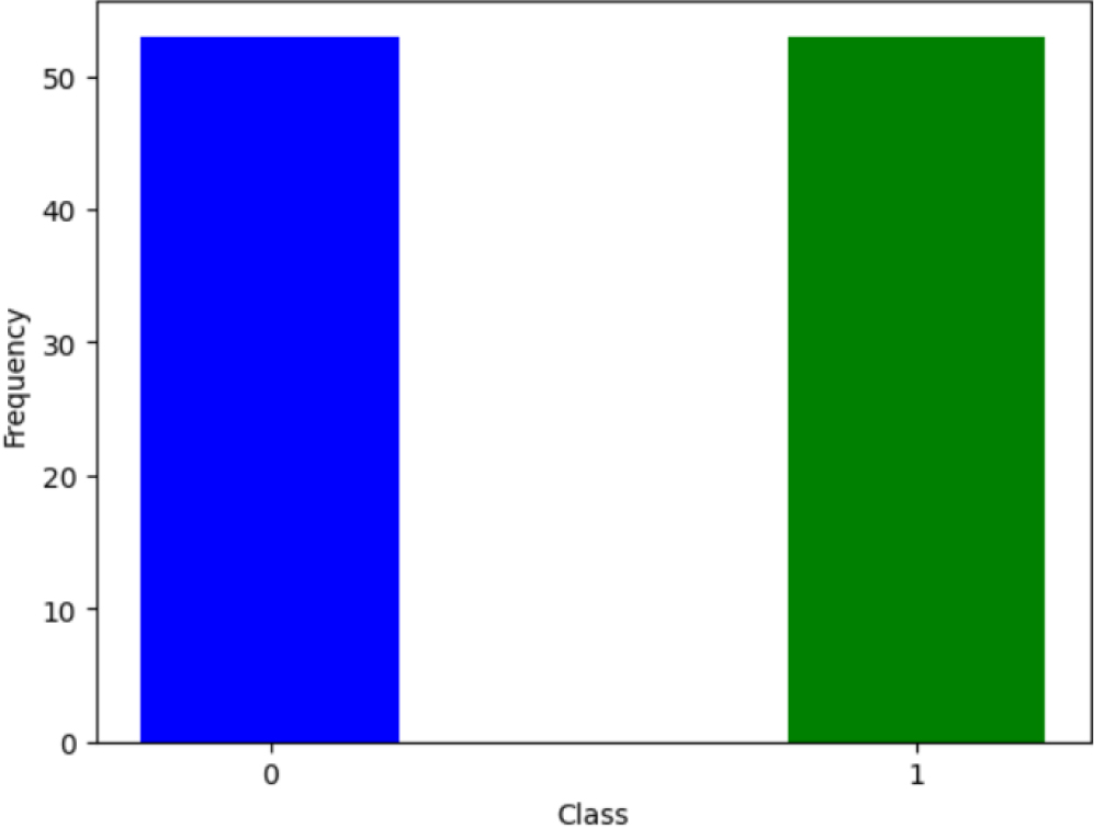

4. Experimental analysis

This research endeavour is executed using Python version 3.10.10. For the classification of DNA sequences, the Scikit-learn library, a comprehensive Python machine learning package offering diverse classification, regression, and clustering techniques, is employed. In addition to that, the NumPy and Pandas libraries are utilized for dataset preprocessing. The versions of the libraries utilized are Numpy: 1.23.5, SKlearn:1.2.2 and Pandas:1.5.3.

The PolynomialFeatures in scikit-learn was the tool used for generating new features by creating polynomial combinations of existing numerical features. It was useful for capturing the non-linear relationships in data. SelectKBest is a feature selection technique provided by scikit-learn (sklearn.feature_selection). It selected the top k most important features from the dataset based on a scoring function. f_classif is one of the scoring functions available for this purpose, and it’s specifically designed for classification tasks. The classification report from scikit-learn was significant because it provides a concise summary of key classification metrics for a machine learning model. It included crucial information such as precision, recall, F1-score, and support for each class.

4.1 Dataset collection and processing

At the outset, the primary dataset encompassed 106 DNA sequences, accompanied by their respective textual class labels denoted as either positive ( $+$ ) or negative ( $-$ ). The dataset comprised 53 promoter sequences and an equal number of non-promoter sequences. Subsequently, a data preprocessing procedure involved disassembling the DNA sequences into individual nucleotides, followed by the application of one-hot encoding on the textual data. As a result, the textual data is effectively transformed into numerical data, wherein each categorical column within the DataFrame underwent replacement by a series of binary columns, thus facilitating further analysis and processing.

Figure 6.

Feature correlation matrix.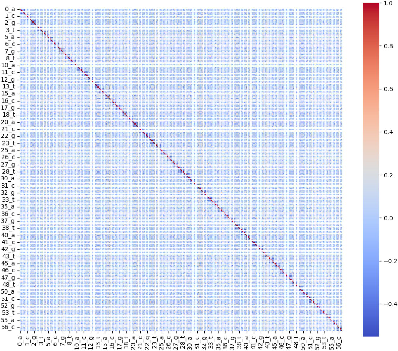

4.2 Feature selection

The computation of scores for each of the 26,334 features is performed through the utilization of the $f\_\textit{classif}$ score function. Subsequently, a stringent selection criterion is employed to identify the top 1000 features, characterized by the highest scores, which are then designated as the input data for further analysis.

Figure 7.

Score of each feature using f_classif function.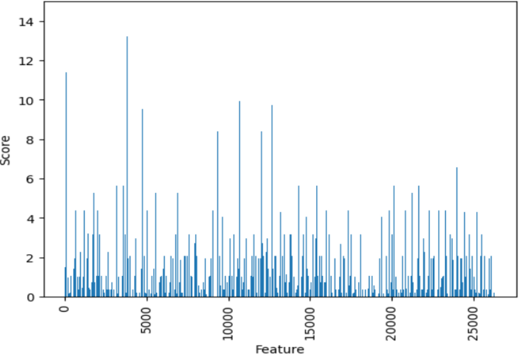

Figure 8.

Selected features (Top 1000).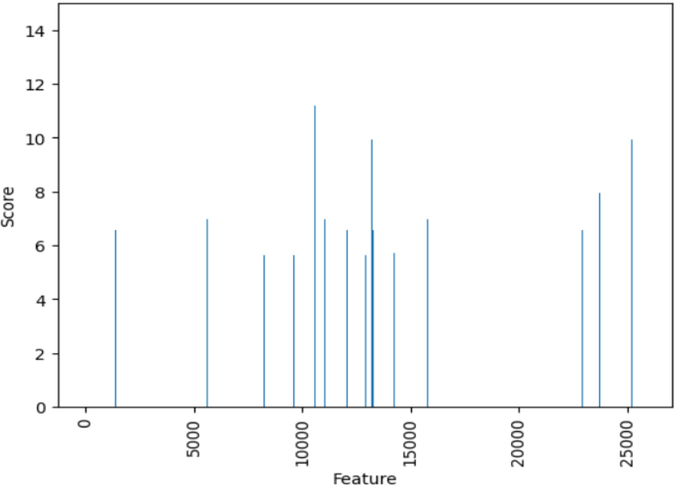

4.3 Gaussian decision boundary estimation

The proposed study employs the Gaussian Decision Boundary Estimator, with the Regularization parameter (C) set to 1.0. Following the training of the Gaussian Decision Boundary Estimator using the selected features, it is subjected to testing. The test dataset comprises 32 sequences, with an equal distribution of 16 promoters and 16 non-promoters. A comparative evaluation is conducted against various alternative machine learning models, including K-Nearest Neighbours (KNN), Gaussian Process Classifier, Decision Tree, Random Forest, Multilayer Perceptron (MLP), AdaBoost, and Naïve Bayes. Notably, the proposed model demonstrated superior performance, achieving an accuracy of 99.9%, as visually depicted in Fig. 10.

Figure 9.

Classification report.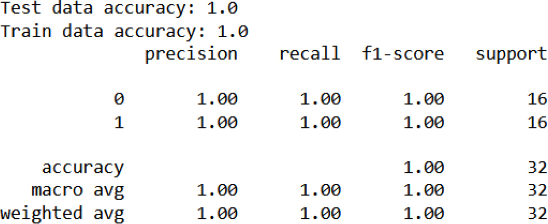

4.4 Assessment of predictive ability

Figure 10.

Confusion Matrix and ROC curve for the proposed model, KNN, MLP, Gaussian, Naïve Bayes, SVM (Linear kernel) and AdaBoost.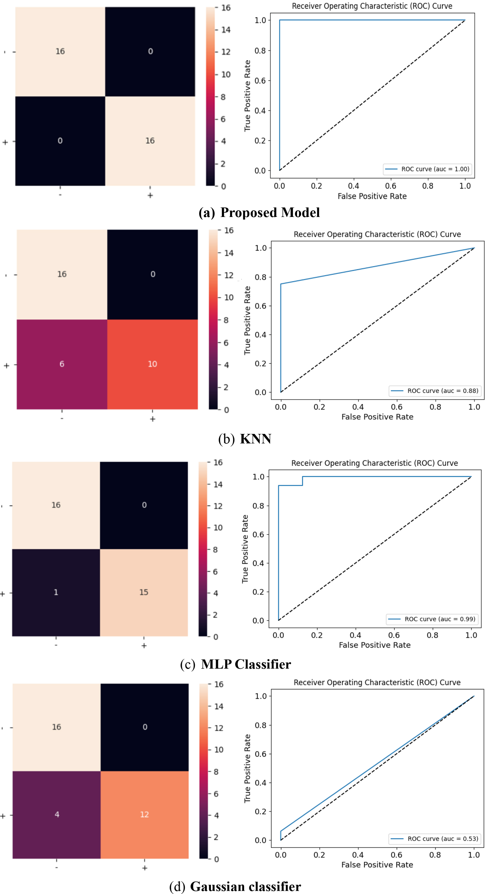

Figure 10.

continued.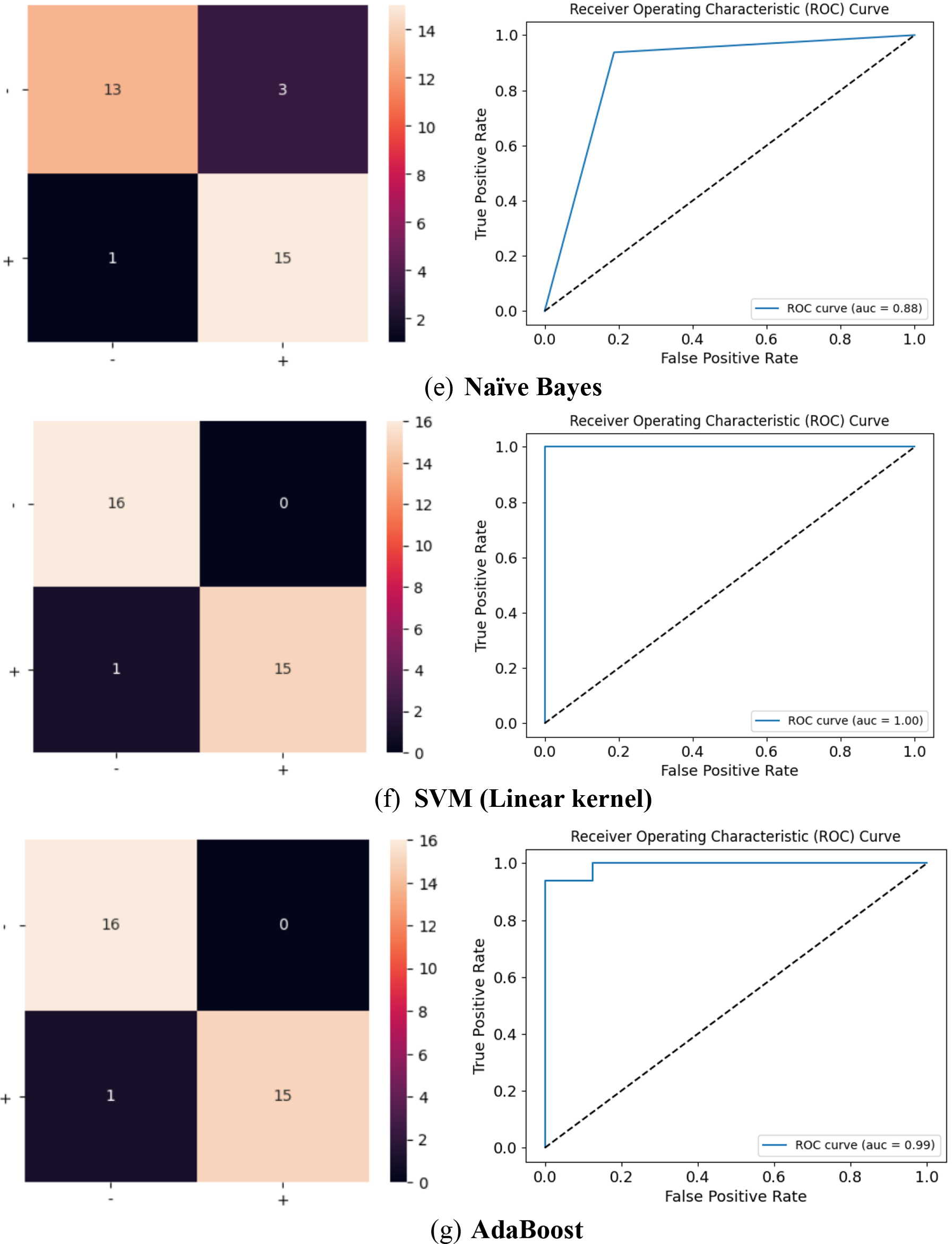

Figure 11.

Comparison of the proposed algorithm with other models.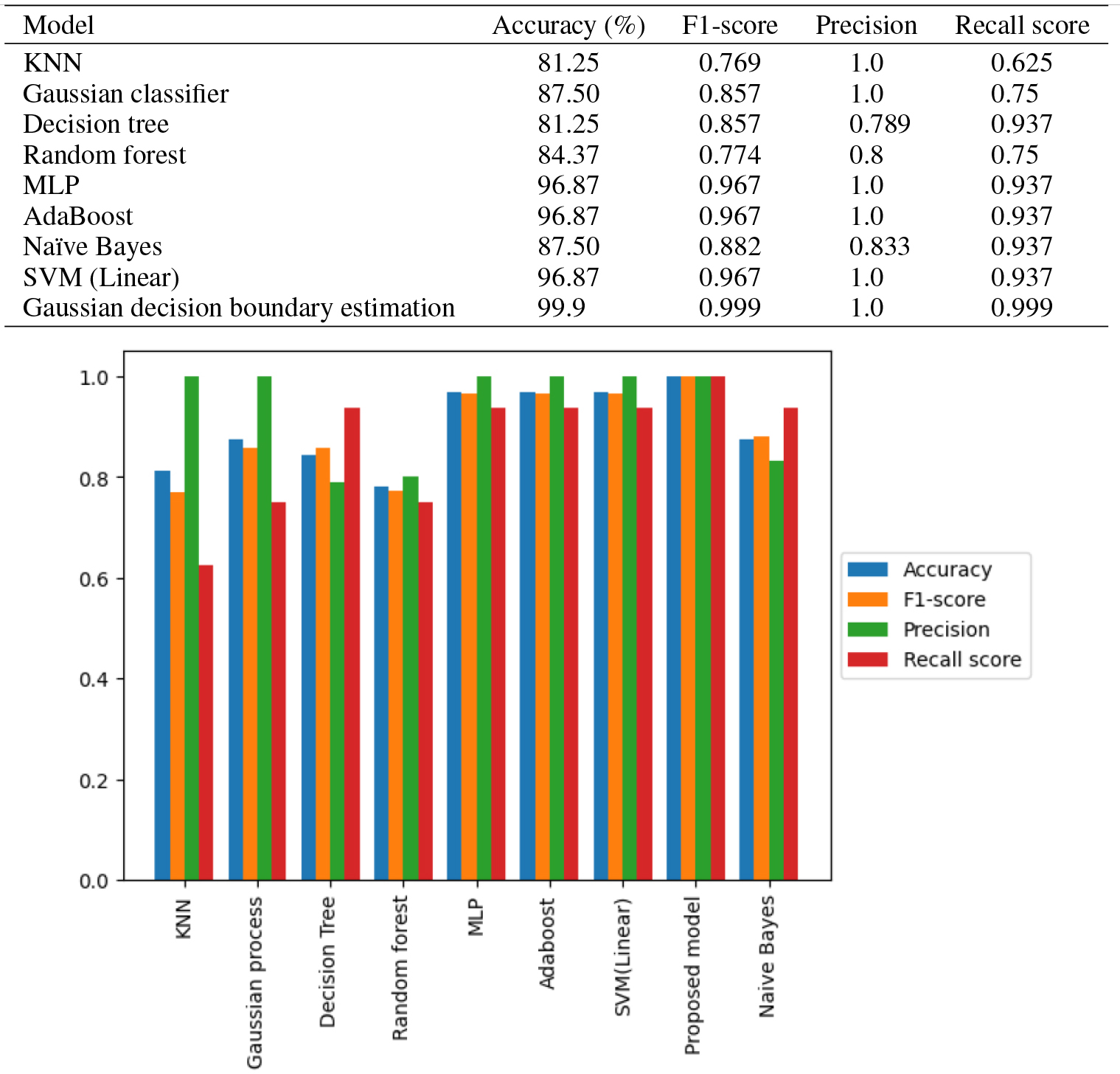

Accuracy, a widely adopted metric in classification performance assessment, delineates the ratio of correctly classified instances to the overall number of instances under consideration. The $\textit{accuracy}\_\textit{score}$ function, an integral component of the sklearn.metrics module, serves the purpose of evaluating the precision of a machine learning model’s predictions.

Mathematically, the accuracy (Acc) can be defined as:

$\displaystyle\textit{Acc}=\frac{\textit{TP}+\textit{TN}}{\textit{TP}+\textit{% TN}+\textit{FP}+\textit{FN}}$

Where,

TP – number of true positives (correctly predicted positive instances).

TN – number of true negatives (correctly predicted negative instances).

FP – number of false positives (incorrectly predicted positive instances, also known as Type I errors).

FN – number of false negatives (incorrectly predicted negative instances, also known as Type II errors).

The F1 score serves as another widely adopted performance metric for evaluating the efficacy of machine learning models, particularly in the context of binary classification tasks. It acts as a harmonizing factor, striking a balance between precision and recall, thereby furnishing a singular measurement that encompasses both aspects.

Mathematically, the F1 score can be defined as:

$\displaystyle F1=2\times\frac{\textit{precision}\times\textit{recall}}{\textit% {precision}+\textit{recall}}$

$\displaystyle\textit{precision}=\frac{\textit{TP}}{\textit{TP }+\textit{FP}}$

$\displaystyle\textit{recall}=\frac{\textit{TP}}{\textit{TP}+\textit{FN}}$

The F1 score exhibits a numerical range from 0 to 1, wherein 1 represents the optimal score, denoting flawless precision and recall. A heightened F1 score indicates a more equitable equilibrium between precision and recall, thereby suggesting superior overall model performance. Moreover, the F1 score imposes a penalty on models that disproportionately prioritize precision or recall, facilitating a more equitable assessment of the model’s capacity to render accurate positive predictions while minimizing the omission of actual positive instances.

The Receiver Operating Characteristic (ROC) curve and its associated metric, the Area Under the Curve (AUC), assume pivotal significance in the appraisal of machine learning modules, particularly those tasked with binary classification. The ROC curve, portrayed graphically, elucidates the relationship between true positive rate (TPR) and false positive rate (FPR) at distinct classification thresholds, facilitating a nuanced understanding of the sensitivity-specificity trade-off. Subsequently, the AUC, a scalar value derived from the ROC curve, quantifies the model’s overall discriminatory prowess.

An AUC value approaching unity signifies exemplary performance, while an AUC of 0.5 conveys chance-level prediction. The amalgamation of the ROC curve and AUC confers a comprehensive evaluation of the classification model’s proficiency in discerning between positive and negative instances, rendering them indispensable tools for model selection, comparative analysis, and informed decision-making across diverse machine learning applications. The Confusion matrix and Receiver operating characteristic curve of various models are shown in Fig. 10.

The Area Under the Receiver Operating Characteristic (ROC) Curve (AUC) for the proposed model signifies its outstanding discriminative capability, displaying exceptional performance in effectively distinguishing between the promoter and non-promoter classes. The ROC curve analysis yields insights into the model’s high discriminatory ability, minimal misclassification, excellent predictive power, strong class separation, and reliable ranking of predictions. Figure 11 shows the comparative analysis of the proposed algorithm with other state of art algorithms.

The confusion matrix is a fundamental tool for assessing the performance of a classification model. It provides insights into the model’s strengths and weaknesses, helping practitioners make informed decisions about model selection and optimization. It’s particularly useful in situations where the consequences of false positives and false negatives are different. The confusion matrix provides a comprehensive and quantifiable assessment of how well the model is performing, and offers insights into the model’s strengths and weaknesses, helping to identify where it excels and where it may need improvement.

The ROC curve of MLP and AdaBoost classifiers infers that it is performing very well. It’s characterized by a steep rise in the TPR (True Positive Rate) while maintaining a low FPR (False Positive Rate) for most classification thresholds. The step in the top left corner indicates near-perfect performance for a range of thresholds. The Area Under Curve is close to the maximum value, suggesting that these classifiers have a high probability of correctly ranking positive instances higher than negative ones, which is a good sign.

The ROC curve of the proposed model, shows a very positive sign of the model’s extremely performance. Additionally, an AUC (Area Under the Curve) value of 0.999 indicates exceptionally high discrimination ability. The shape of curve indicates that the model can effectively distinguish between positive and negative instances with minimal misclassification. This is a strong indication of a well-trained and well-performing classification model.

5. Conclusion

The current realm of research is prominently focused on the utilization of diverse data mining technologies encompassing data mining architecture, the development of ML algorithms, and the exploration of novel data mining analysis functions, tailored for biological information processing. Within this context, an extensive comparison of multiple methods for promoter detection in nucleotide sequences has been undertaken. The unequivocal findings underscore the considerable advantages of the proposed approach, exhibiting a remarkable accuracy of 99.9% on the identical dataset, surpassing the efficacy of existing methodologies. In the fields of bioinformatics and genetics, the classification of promoters from DNA sequences has a variety of applications, including understanding gene regulation, disease research, precision medicine, and bioinformatics research.

References

Liu

Yang

Huang

Chou

. iPromoter-2L: a two-layer predictor for identifying promoters and their types by multi-window-based PseKNC. Bioinformatics. 2018 Jan 1; 34(1): 33-40. doi: 10.1093/bioinformatics/btx579.

Watson

Crick

. Molecular structure of nucleic acids: a structure for deoxyribose nucleic acid. Nature. 1953 Apr 25; 171(4356): 737-8. doi: 10.1038/171737a0.

Wolfsberg

McEntyre

Schuler

. Guide to the draft human genome. Nature. 2001 Feb 15; 409(6822): 824-6.

Burgess

Travers

Dunn

Bautz

. Factor stimulating transcription by RNA polymerase. Nature. 1969 Jan 4; 221(5175): 43-6. doi: 10.1038/221043a0.

Travers

Burgess

. Cyclic re-use of the RNA polymerase sigma factor. Nature. 1969 May 10; 222(5193): 537-40. doi: 10.1038/222537a0.

Fickett

Hatzigeorgiou

. Eukaryotic promoter recognition. Genome Research. 1997 Sep 1; 7(9): 861-78. doi: 10.1101/gr.7.9.861.

Pedersen

Baldi

Chauvin

Brunak

. The biology of eukaryotic promoter prediction – a review. Computers & Chemistry. 1999 Jun 15; 23(3-4): 191-207. doi: 10.1016/S0097-8485(99)00015-7.

Khan

Arya

Kanumuri

. Promoter identification in DNA sequences using machine learning. In 2020 IEEE 17th India Council International Conference (INDICON) 2020 Dec 10 (pp. 1-4). doi: 10.1109/INDICON49873.2020.9342360.

Rani

Bhavani

Bapi

. Analysis of E. coli promoter recognition problem in dinucleotide feature space. Bioinformatics. 2007 Mar; 23(5): 582-8. doi: 10.1093/bioinformatics/btl670..

10.

Werner

. The state of the art of mammalian promoter recognition. Briefings in Bioinformatics. 2003 Mar 1; 4(1): 22-30. doi: 10.1093/bib/4.1.22.

11.

Altschul

Gish

Miller

Myers

Lipman

. Basic local alignment search tool. Journal of molecular biology. 1990 Oct 5; 215(3): 403-10. doi: 10.1016/S0022-2836(05)80360-2.

12.

Towell

Shavlik

Noordewier

. Refinement of approximate domain theories by knowledge-based neural networks. In Proceedings of the eighth National conference on Artificial intelligence-Volume 2; 1990 Jul 29 (pp. 861-866).

13.

Weinert

Lopes

. Neural networks for protein classification. Applied Bioinformatics. 2004 Mar; 3: 41-8. doi: 10.2165/00822942-200403010-00006.

14.

Gordon

Towsey

Hogan

Mathews

Timms

. Improved prediction of bacterial transcription start sites. Bioinformatics. 2006 Jan 15; 22(2): 142-8.

15.

Tavares

Lopes

Erig Lima

. A comparative study of machine learning methods for detecting promoters in bacterial DNA sequences. In Advanced Intelligent Computing Theories and Applications. With Aspects of Artificial Intelligence: 4th International Conference on Intelligent Computing, ICIC 2008 Shanghai, China, September 15–18, 2008 Proceedings 4 2008 (pp. 959-966). Springer Berlin Heidelberg. doi: 10.1007/978-3-540-85984-0_115.

16.

Abeel

Saeys

Bonnet

Rouzé

Van de Peer

. Generic eukaryotic core promoter prediction using structural features of DNA. Genome research. 2008 Feb 1; 18(2): 310-23.

17.

Zhang

. A novel promoter prediction method inspiring by biological immune principles. In 2009 WRI Global Congress on Intelligent Systems 2009 May 19 (Vol. 1, pp. 569-573). IEEE.

18.

Polat

Güneş

. A new method to forecast of Escherichia coli promoter gene sequences: Integrating feature selection and Fuzzy-AIRS classifier system. Expert Systems with Applications. 2009 Jan 1; 36(1): 57-64. doi: 10.1016/J.ESWA.2007..

19.

Karlı

. Promoter prediction using IREM (inductive rule extraction method). vol. 3(1), 2014. Available from: http//www.ijerst.com/currentissue.php.

20.

Anveshrithaa

Aathavan

Jaisankar

. Promoter prediction in DNA sequences of escherichia coli using machine learning algorithms. International Journal of Scientific and Technology Research. 2019; 8(11): 3000-4.

21.

Frank

. UCI machine learning repository. http://archive.ics.uci.edu/ml. 2010. Available from: http//archive.ics.uci.edu/ml/.

22.

Kallimani

. Machine Learning Based Predictive Action on Categorical Non-Sequential Data. Recent Advances in Computer Science and Communications (Formerly: Recent Patents on Computer Science). 2020 Oct 1; 13(5): 1020-30. doi: 10.2174/2213275912666190417150421.

23.

Kramer

. Scikit-learn. Machine learning for evolution strategies. 2016; 45-53. doi: 10.1007/978-3-319-33383-0_5.

24.

Pedregosa

Varoquaux

Gramfort

Michel

Thirion

Grisel

Blondel

Prettenhofer

Weiss

Dubourg

Vanderplas

. Scikit-learn: Machine learning in Python. The Journal of Machine Learning Research. 2011 Nov 1; 12: 2825-30.

25.

Mishra

Singh

Pandey

Mishra

Pandey

. Application of student’s t-test, analysis of variance, and covariance. Annals of Cardiac Anaesthesia. 2019 Oct; 22(4): 407. doi: 10.4103/aca.ACA_94_19.

26.

Burges

. A tutorial on support vector machines for pattern recognition. Data Mining and Knowledge Discovery. 1998 Jun; 2(2): 12167. doi: 10.1023/A1009715923555.

27.

Han

Pei

Tong

. Data mining: concepts and techniques. Morgan Kaufmann. 2022 Jul 2.

Classifying promoters by interpreting the hidden information of DNA sequences for disease prediction in clinical laboratories using Gaussian decision boundary estimation

Abstract

Keywords

1. Introduction

Table 1 Comparison of proposed model with other state of art algorithms

3.3 Feature selection using f ⁢ _ ⁢ 𝑐𝑙𝑎𝑠𝑠𝑖𝑓 score function

3.4 Gaussian decision boundary estimation

4.1 Dataset collection and processing

References

Table 1
Comparison of proposed model with other state of art algorithms

3.3 Feature selection using $f\_\textit{classif}$ score function