Sage Journals: Discover world-class research

Abstract

The performance of Adaboost is highly sensitive to noisy and outlier samples. This is therefore the weights of these samples are exponentially increased in successive rounds. In this paper, three novel schemes are proposed to hunt the corrupted samples and eliminate them through the training process. The methods are: I) a hybrid method based on K-means clustering and K-nearest neighbor, II) a two-layer Adaboost, and III) soft margin support vector machines. All of these solutions are compared to the standard Adaboost on thirteen Gunnar Raetsch’s datasets under three levels of class-label noise. To test the proposed method on a real application, electroencephalography (EEG) signals of 20 schizophrenic patients and 20 age-matched control subjects, are recorded via 20 channels in the idle state. Several features including autoregressive coefficients, band power and fractal dimension are extracted from EEG signals of all participants. Sequential feature subset selection technique is adopted to select the discriminative EEG features. Experimental results imply that exploiting the proposed hunting techniques enhance the Adaboost performance as well as alleviating its robustness against unconfident and noisy samples over Raetsch benchmark and EEG features of the two groups.

Keywords

Class-label noise noise pruning AdaBoost margin theory support vector machines

1. Introduction

The performance of conventional classifiers heavily relies on being trained with correctly-labelled datasets. However, in practice, labels of training samples can be corrupted by expert mistakes [20, 26, 45], encoding errors [22, 37], and poor quality of recorded data [8]. To overcome this deficiency, two general solutions have been proposed in the literature. The first approach has focused on making specific supervised learning algorithms robust to mislabelled samples [34] while the other approach has concentrated on finding and removing noisy samples as a pre-processing step prior to learning [7, 31]. The second approach benefits from independence to the type of classifier. In other words, these methods are general and can be used for improving the performance of a wide range of classifiers. Therefore, this study is focused to develop some new techniques within the framework of the second approach.

Contrary to the common belief that having more training data necessarily increases the generalization of all classifiers, studies conducted by [7] showed that the classifiers’ efficacy might be better off when noisy examples are discarded from the training set. To some extent, the quality of training data is more important than its quantity. Therefore, pruning noisy and unconfident samples from training data, is the first necessary step to achieve a better generalization.

Adaptive boosting (Adaboost) is proposed by [16] and has become the most famous ensemble learning algorithm due to its strong statistical background [19]. Adaboost is able to finely handle missing values with minimum information loss, in addition to providing enough flexibility to construct every complex border by linear combination of simple classifiers [12, 25]. These properties along with its fast execution placed it among the top ten machine learning algorithms. However, the main flaw of AdaBoost appears when it boosts the importance of noisy and unconfident samples across its successive weak learners [27]. This boosting is a result of the sample-weighting rule, which increases the weight of hard-to-classify samples continually in a way that learners are biased to the noisy and outlier samples, which are misclassified across successive learners [21].

Several attempts have been made to remove the noisy and outlier samples, as a pre-processing step for Adaboost. [10] used both Gini impurity and one-class SVM methods in order to estimate the best partitioning, in which the percentage of noise filter ratio is maximized. After eliminating the noisy samples, an Adaboost was applied to classify each partition. Nevertheless, this method cannot adaptively set the filtering parameters. In another attempt [48] tried to eliminate the noisy (confusing) samples by a Bayesian-like classifier in an iterative manner. This is done by minimizing the defined average loss of the Bayesian-like classifier. This approach does not need any prior knowledge and covariance matrix estimation. Despite its efficient mathematical derivation, this method eliminates a high portion of samples, which are laid in the margin of classes.

In this study, three novel schemes were proposed to detect induced class-label noises in various datasets using: 1) a hybrid approach based on K-means clustering and K-nearest neighbor, 2) a two-layer AdaBoost, and 3) using soft margin Support Vector Machine (SVM). The effectiveness of the three proposed filtering methods were tested on Adaboost.M1, which is a well-known noise sensitive classifier.

The rest of this paper is structured as follows: Section 2 presents the methodology, including a detailed explanation of AdaBoost and the three proposed methods for the noise filtering. Section 3 presents evaluation criteria and describes the employed data sets. In Section 4, the results of the solutions and their pros and cons are discussed. The paper is finally concluded and some notes, as the future work, are presented in Section 5.

2. Method

In this section, first, the Adaboost algorithm is described and the reason for its sensitivity to noisy samples/labels is finely explained. Afterward, the proposed filtering methods are introduced.

2.1 Adaboost

Ensemble learning refers to training a collection of individual learners, which are connected in a serial, parallel or other structures to map inputs to outputs. The idea behind the ensemble learning is very innovative: the combination of weak learners can act better than a strong single learner [9]. In contrast to the conventional classifiers that use the classification error as their feedback to update their parameters, Adaboost assigns a weight to each sample and defines a pseudo-loss function that plays the role of error [44]. The value of this loss function for each learner is determined by the summation of the weights of misclassified samples. The name of Adaboost stands for “Adaptive Boosting” because it boosts the weight of misclassified samples and decreases the weights of correctly classified samples. In fact, a simple base learner (weak learner) is selected and is sequentially trained by different weighting distribution of samples while in the recall phase, all of the trained weak learners are activated in parallel and their outputs are fused by a linear weighting combination [16]. The distribution of samples’ weight of the $t^{\text{th}}$ leaner, denoted by $D_{t}(.)$ , is updated according to the following formula:

$\displaystyle D_{t+1}(i)=\frac{D_{t}(i)\ast\exp({-\alpha_{t}y_{i}h_{t}({x_{i}}% )})}{Z_{t}}$ (1)

where $h_{t}(x)$ indicates the output of hypothesis (learner) at iteration $t$ , the multiplier $a_{t}$ shows the weight of each learner’s output, $y_{i}$ is the true label of the sample $x_{i}$ and $Z_{t}$ is the normalization factor to ensure that the weights sum to 1. According to the formula, If $h_{t}({x_{i}})$ correctly classified example $x_{i}$ (i.e., if $y_{i}h_{t}({x_{i}})$ is positive), then the factor is less than 1, and the weight $D_{t}(i)$ is decreased. This means that the example $x_{i}$ will have less influence on the next weak classifier trained in the next iteration, because it was already classified correctly by the current weak classifier. On the other hand, if $h_{t}({x_{i}})$ misclassified example $x_{i}$ (i.e., if $y_{i}h_{t}({x_{i}})$ is negative), then the factor is greater than 1, and the weight $D_{t}(i)$ is increased. This means that example $x_{i}$ will have more influence on the next weak classifier trained in the next iteration, because it was misclassified by the current weak classifier.

The factor in the weight update formula is controlled by the parameter $\alpha_{t}$ , which is computed based on the error rate of the weak classifier $h_{t}(x)$ on the training examples. The larger the error rate, the smaller the value of $\alpha_{t}$ , and the smaller the influence of $h_{t}(x)$ on the final classifier. Conversely, the smaller the error rate, the larger the value of $\alpha{\_}t$ , and the larger the influence of $h_{t}(x)$ on the final classifier. The overall effect of this weight update procedure is to focus the attention of the subsequent weak classifiers. on the examples that are harder to classify correctly, while ignoring the examples that are easier to classify. This leads to a final classifier that is more accurate than any of the individual weak classifiers.

Figure 1.

Final distribution of samples’ weight assigned by AdaBoost on Breath Cancer data samples after 100 iterations.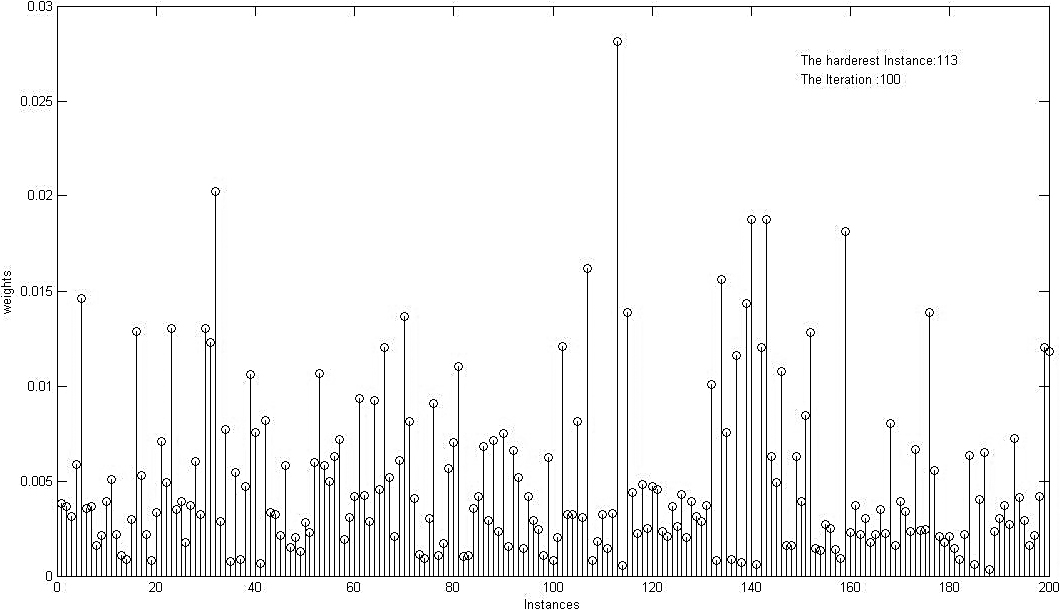

According to Eq. (1), the weight of a noisy or unconfident sample, which is hard-to-classify in essence, would increase repeatedly over the successive iterations. Consequently, the decision boundaries of last base learners would be dragged toward the noisy samples and therefore disturbs the final decision boundary of the overall classifier. An example of the final weight distribution of Adaboost is illustrated Fig. 1. As shown, some samples gain much larger weight compared to others.

2.2 Proposed filtering methods

In this section, three different solutions are proposed for hunting noisy and unreliable samples. What follows, is the descriptions of these methods in a comprehensive manner.

2.2.1 Combination of K-means & KNN

AApplying a clustering algorithm for outlier detection is a common approach, where outlier samples are defined as those with a low number of neighbors in their vicinity. To enhance the identification of outlier points, the density distribution of all samples (regardless of their labels) is estimated, and samples located far from dense regions are removed. For instance, the K-nearest neighbor (KNN) method is iteratively used to detect noisy samples that assign incorrect labels to the neighbors [31].

On the other hand, the traditional clustering approach for outlier detection suffers from scarifying (e.g., deleting) samples around the hypothetical decision boundary. For instance, the application of KNN to marginal samples enables the detection and deletion of those samples that provide incorrect labels for the neighbors. However, this deletion has the potential to disrupt the hypothetical boundary between classes, leading to an underestimation of classifier parameters [42]. Hence, it is necessary to exclusively apply KNN to specific regions. To achieve this objective, a new concept called “sole sample” is introduced, defined as follows: a sample within a cluster (consisting of at least three samples) is referred to as a sole sample if its label differs from its neighbors within the same cluster.

Figure 2.

Illustration of “sole samples” (potential noises) and outliers in a hypothetical two-class classification problem.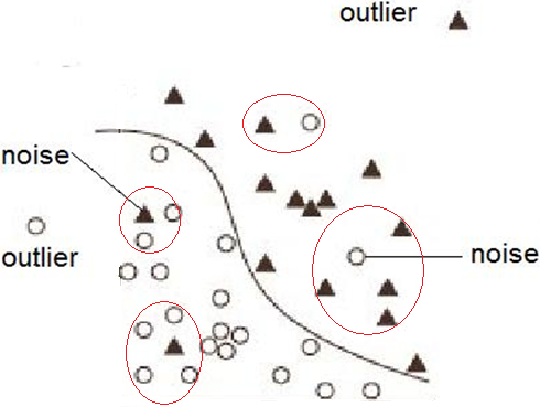

Figure 2 clarifies the concept of sole sample in a two-dimensional space for a hypothetical two-class problem. The underlying assumption is that a sample is less likely to be “sole” when it is close to the decision boundary.

In this study, a hybrid scheme combining both supervised and unsupervised approaches is proposed to better detect the noisy samples. First, a subtractive clustering is applied to the whole data (without considering their label) for estimating the distribution of data. Subtractive clustering is a type of clustering algorithm that uses a density function to determine the number and locations of clusters in a dataset. The main idea behind subtractive clustering is to first find the potential centers of the clusters, and then assign data points to the nearest cluster center based on their distance. The pseudocode for the algorithm can be found following:

Input: Data set X, Distance function d, Influence radius R, Threshold T

1. Initialize the list of clusters C as empty

2. Calculate the initial density of each point in X using the distance function d and the influence radius R

3. Sort the points in X by their density in descending order

4. Take the first point x1 with the highest density and add it to a new cluster c1

5. For each remaining point xi in X, do the following:

a. Calculate the distance between xi and each point in the cluster ci using the distance function d

b. Calculate the density of xi based on the distances and the influence radius R

c. If the density of xi is greater than the threshold T, add xi to the cluster ci

d. Otherwise, create a new cluster ci

+

1 with xi as its initial point

6. Repeat steps 4–5 until all points in X have been assigned to a cluster

7. Output the list of clusters C

Subtractive clustering has some advantages over other clustering algorithms. It can automatically determine the number of clusters in a dataset, which can be useful when the number of clusters is not known in advance. Additionally, it is computationally efficient, as it does not require an iterative optimization process like some other clustering algorithms.

Second, by exploring through the search space, centers of dense regions are considered as initial centers of clusters in the $K$ -means algorithm [47]. After running $K$ -means using the initialized centers, appropriate clusters are created. Now, sole samples within each cluster are detected according to the mentioned scheme. To correct the unconfident and noisy samples, KNN ( $K=$ 5) is applied to samples of each cluster in order to manipulate the sole samples by eliminating or relabeling them, depending on the adopted policy in the proposed algorithm.

Estimating both the appropriate number of clusters along with their initial centers plays the key role in the performance of $K$ -means. In this research, subtractive clustering [11] is applied to data for estimating the number and location of clusters’ centers.

Subtractive clustering is a fast and one-pass algorithm which has been repeatedly used to estimate the distribution of input data [11]. When appropriate distribution is estimated, as mentioned before, the number of dense regions along with their centers are estimated as the primary centers. This method assumes that the data falls within a unit hypersphere. It has only one user-defined parameter, as the average radius of neighborhood (RADII). This parameter theoretically ranges from 0 to 1 while in practice a value between 0.2 and 0.5 is deployed. Considering small values for RADII results in a high number of small clusters and vice versa. After finding a cluster center in the subtractive clustering, all samples within the RADII around this center are subtracted from the dataset in order to determine the next cluster center. This process is repeated until all of the data is removed.

Defining clusters’ centers with this method has the great advantage of stability compared to conventional random initialization of cluster centers.

As previously defined, sole samples can only be found in clusters with at least three samples. Therefore, over-emphasizing the locality of data (i.e. smaller RADII) produces a large number of small clusters (micro-cluster) with one or two samples. Thus, it leads to a considerable portion of noisy samples. On the other hand, as the size of a potential cluster grows, it is more likely to contain multiple samples from different classes; however, meeting the singularity condition for being a sole sample in a cluster is less likely to be satisfied.

For instance, in a hypothetical 100-sample training dataset, finding a “sole sample” in a cluster containing %10 the all data requires having 9 samples from the same class in a cluster. This scenario would be much less likely than finding a sole sample in a cluster with only %5 of data (i.e. only 4 samples from the same class in a cluster). For this reason, RADII is set to 0.5 in order to hold the maximum size of clusters to %5 of the overall training set.

When a sole sample is detected, two policies can be adopted: deletion and correction. Deletion of the samples means removing some information from the training data which can lead to weakening the learning process. On the other hand, the correction approach has the risk of creating noisy samples in training data, particularly in multi-class problems. However, in the case of having a two-class classification problem, this risk can be managed by setting a low value for the ratio of detected sole samples to the whole training data. In addition, the percentage of noisy samples to sole samples should be acceptable. In Section 4, the achieved experimental results illustrate that the performance of deletion policy can be further improved by “correcting” the labels of “mislabelled” samples and then executing the clustering phase again. Figure 3 illustrates the flowchart of the presented clustering method.

Figure 3.

General schema of clustering solution.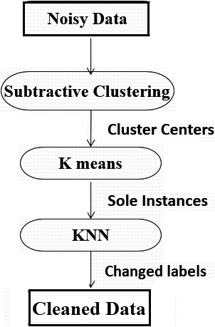

2.2.2 Noise filtering using adaptive boosting

It is intuitive that the most detrimental-to-learning noises are among those samples that have gained highest weights during the Adaboost learning process. Therefore, pruning samples with high weight can be considered as a method for removing noisy samples. Since the Adaboost learning process is a sequential procedure, relying just on the final distribution of weights is misleading [13]. It cannot be ruled out that a noisy sample with a relatively low weight, in the final distribution, exerts its negative effect on first few base learners and then being correctly classified by the last base learners.

To address this issue, the weights of samples are investigated through each epoch of AdaBoost, and then a frequency-based approach is employed to define “hard samples”. In other words, a group of “suspected-to-noise” samples is detected regarding their weights’ distribution. To detect these samples, a threshold is defined, and those weights above this value are considered as the suspected ones. The threshold value is defined as follows:

$\displaystyle\textit{Tereshold}_{t}=\textit{Mean}({\textit{weight}_{t}})+% \textit{Std}({\textit{weight}_{t}})$ (2)

where $t$ is the iteration number, ranging from 1 to $T$ . After the last iteration of the algorithm ( $T$ ), all the samples presented in the T suspected groups are sorted based on their frequency of appearing among suspected instances. Regarding a pre-defined “Pruning rate”, the top frequent samples would be removed from the dataset as noisy samples. The general schema of the proposed AdaBoost Filtering algorithm is illustrated in Fig. 4. It should be noted that assigning a large value to “Pruning rate” would probably increase the chance of eliminating critically important samples, which are not certainly noisy. In the setup, the “Pruning rate” is set to %5, indicating that only the top %5 of the most frequent suspected samples would be removed.

Figure 4.

General schema of AdaBoost filtering.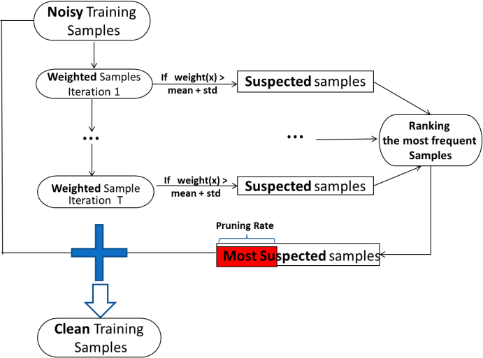

Our preliminary results showed that in the AdaBoost filtering method, unlike cluster-based filtering, a notable percentage of training data is defined as suspected noisy samples. Therefore, flipping the labels of the suspected noises has the risk of inducing new noises into the training set. Nevertheless, there is no way to guarantee that the effect of potential noises induced by the correction policy is less harmful than that of the original random noises. For this reason, the deletion policy was selected as the last stage of this method.

2.2.3 Noise filtering using SVM

Support vector machine (SVM) method tries to maximize the margin width simultaneously by gaining maximum accuracy over training samples. In general, Margin of a sample is defined as the distance of that sample from the decision boundary. To increase the SVM generalization, its margin should be wide as much as possible while it might damage the train result.

Since the SVM boundary is just adjusted by the support vectors, noisy support vectors deteriorate its boundary. Therefore, train samples should be as clean as possible and then enlarging the margin width to increase its robustness against the remained noisy samples (i.e. Soft Margin) [36]. If the boundary between the classes is nonlinear, a kernel is used to enable SVM to form a flexible boundary [30].

SVM considers a cost, in terms of slack variables $\xi_{i}$ , for each example $x_{i}$ , depending on how far it is located from the boundary. If the sample falls within the margin on the correct side of the boundary 0 $<\xi_{i}<$ 1, else if it placed within the margin but on the wrong boundary’s side, $\xi_{i}>$ 1. Hence, the train error is measured by the following inequalities:

$\displaystyle y_{i}({X_{i}^{T}W+b})\geqslant 1-\xi_{i}$

(3) $\displaystyle({i=1,\ldots,m})$

Where $b$ is the bias and $W$ is the hyper-plane between two classes. The SVM optimization problem is defined as:

$\displaystyle\textit{Minimize }W^{T}W+C\mathop{\sum}\limits_{i=1}^{m}\xi_{i}^{k}$ Subject to (4) $\displaystyle y_{i}({X_{i}^{T}W+b})\geqslant 1-\xi_{i}$ $\displaystyle\xi_{i}\geqslant 0({i=1,\ldots,m})$

Here $C$ is a regularization parameter, which controls the trade-off between maximizing the margin and minimizing the training error. $K$ determines the order of norm that will be explained later. A small $C$ tends to emphasize the margin and ignore the outliers in the training data, while a large $C$ may tend to overfit the training data [23]. In all of the later-shown results in this paper, the value of C was set to 1.

According to the above explanations, two types of soft margin SVMs can be defined: L1-norm ( $k=$ 1) which is based on a linear sum of slack variables and L2-norm ( $k=$ 2) which is based on a square sum of slack variables [24]. Solving the optimization problem of L1-Soft Margin would finally lead to following equations:

$\displaystyle 0<a_{i}<C\to y_{i}({X_{i}^{T}W+b})=1$ $\displaystyle a_{i}=0\to y_{i}({X_{i}^{T}W+b})\geqslant 1$ (5) $\displaystyle a_{i}=C\to y_{i}({X_{i}^{T}W+b})\leqslant 1$

where $a_{i}$ is the Lagrangian coefficient of $i^{\text{th}}$ sample and $C$ is its upper bound. According to Eq. (2.2.3), there is no difference among Lagrangian coefficients of misclassified samples. When L2-norm is used, the condition $\xi_{i}\geqslant 0$ is dropped. The primal Lagrangian for the L2-norm problem is:

$\displaystyle L_{p}({W,b,\xi,a})=\frac{1}{2}W^{T}W+\frac{C}{2}\mathop{\sum}% \limits_{i=1}^{m}\xi_{i}^{2}$ $\displaystyle-\mathop{\sum}\limits_{i=1}^{m}a_{i}[{y_{i}({W^{T}X+b})-1+\xi_{i}}]$ (6) Subject to $\displaystyle y_{i}({X_{i}^{T}W+b})\geqslant 1-\xi_{i}({i=1,\ldots,m})$

The derivations of Eq. (2.2.3) with respect to $b$ and $\xi$ would be as follows:

$\displaystyle\frac{\partial L}{\partial w}=W-\mathop{\sum}\limits_{i=1}^{m}y_{% i}a_{i}X_{i}=0;$ (7) $\displaystyle\frac{\partial L}{\partial b}=\mathop{\sum}\limits_{i=1}^{m}y_{i}% a_{i}=0;$ (8) $\displaystyle\frac{\partial L}{\partial\xi}=C\xi-a=0;$ (9)

Equation (9) indicates that in a L2-soft margin SVM, the Lagrangian coefficients ( $a$ ) of each sample is proportional to that sample’s slack value. Therefore, for any data point, being further away from the margin of its own class equates to having a larger Lagrangian coefficient. This is valuable because the Lagrangian coefficient can be extracted from any trained SVM model. While our assumption in this paper is that class-label nosies are uniformly distributed across the training data boundaries, it is obvious that the most detrimental mislabeled samples are the ones who are located far from the boundaries of the two classes as they drag the decision boundary between the two classes toward themselves (see Fig. 7 as an example). Therefore, the decision boundary can be protected against the negative effect of outliers by removing the support vectors with large Lagrangian coefficients.

To implement this approach, a SVM model is first trained on the polluted training data to obtain the estimated Lagrangian coefficients of all support vectors. Then, an appropriate threshold is set, and samples with Lagrangian coefficients higher than the threshold are identified as noisy samples. Based on the results of exploratory experiments, the most effective parameter value was found to be the mean of the estimated coefficients plus one standard deviation. Apparently, having a larger threshold can increase the method precision but will reduce its recall (i.e. less number of the noisy samples would be detected).

It should be noted that unlike L1-soft margin SVM, there is no upper bound for Lagrangian coefficients, which facilitates one of our vital requirements, ranking procedure of mislabelled samples. In addition, it is worth mentioning that the C parameter and the Lagrangian coefficients are related through the optimization problem that is solved by the SVM algorithm. The optimization problem is a constrained quadratic programming problem that involves minimizing the error (or loss) function subject to the constraints that the Lagrangian coefficients are non-negative and sum to 1. The C parameter appears in the constraints as an upper bound on the Lagrangian coefficients, meaning that the Lagrangian coefficients cannot exceed the value of C. Therefore, a larger value of C corresponds to a higher penalty for misclassifying training examples, which results in a narrower margin and more support vectors. A smaller value of C corresponds to a lower penalty for misclassification, which results in a wider margin and fewer support vectors.
3. Evaluation

Codes of all of the presented algorithms were developed using Statistics and Machine Learning Toolbox, MATLAB 2012a. The performance of our proposed methods was tested on a well-known collection of the thirteen benchmark datasets derived from the UCI, DELVE and STATLOG repositories [18]. The dimensions of these data sets vary from 2 to 60, the numbers of training samples are from 140 to 1300 and the numbers of test samples range from 75 to 7000. Covering a wide range of dimensionality and complexity, these datasets have been recommended for model assessment in ensemble and kernel learning methods [36]. Each dataset contains 100 sets of train-tests, except for Splice and Image datasets, which have only 20 splits (see Table 1).

Table 1
Description of the benchmark datasets

Dataset	Number of samples	Number of features	Train set size	Test set size
Banana	5300	2	400	4900
Breast	263	9	200	77
Diabetis	768	8	468	300
FlareSolar	144	9	666	400
German	1000	20	700	300
Heart	270	13	170	100
Image	2086	18	1300	1010
Ringnorm	7400	20	400	7000
Splice	2991	60	1000	2175
Thyroid	215	5	140	75
Titanic	24	3	150	2051
Two norm	7400	20	400	7000
Waveform	5000	21	400	4600
Real EEG	1170	280	870	300

Additionally, EEG signals of twenty schizophrenic patients (mean age 33.3 and standard deviation (std) 9.52) and twenty normal subjects (mean age 33.4 and std 9.29) are considered [38]. The 20-channel EEG signals are partitioned to a number of one-second windows where its dynamics is assumed to be approximately stationary within each window [2, 3]. Successive windows have 50% overlap. Informative features were extracted from all channels in the same window time. In each window, 14 features were extracted that consist of eight autoregressive coefficients, five band power, and Higuchi fractal dimension [39]. Therefore, the data set will have 280 features (20 channel *14 features) for each window. The extracting features are explained in details as follows:

3.1 AR coefficient

The autoregressive (AR) model, which predicts a sample based on the weighted average of its $p$ prior samples, is one of the most effective tools for signal modeling. The relationship shown below models a stationary signal, $x[n]$ :

$\displaystyle x[n]=\sum_{i=1}^{p}\hat{a}_{i}x[n-i]$ (10)

where $p$ determines the model order and $\hat{a}_{i}$ specifies the AR model coefficients. In this study, the total of the forward and backward prediction errors is used to estimate the AR coefficients using the Burg method. Additionally, the residual variance and the prediction error are taken into account when choosing the appropriate order for the AR model using the finite sample criterion [33, 41].

3.2 Band power

It has been demonstrated that the EEG has many frequency components that can display various brain states and carry discriminatory data [14]. EEG is typically divided into five frequency ranges: delta (less than 4 Hz), theta (4–8 Hz), alpha (8–13 Hz), beta (13–30 Hz), and gamma (greater than 30 Hz). The power in these five bands at each electrode site is shown by the band power feature. First, a band-pass filter (Butterworth filter of order 5) filters the signal within predetermined frequency ranges. Second, the average of each sample over a one-second period is squared.

3.3 Higuchi fractal dimension

The degree of irregularity in a signal can be thought of as the fractal dimension [46]. When the original signal is seen as a geometric figure, it immediately calculates the fractal dimension in the time domain. Following steps outlines the method used to calculate the Higuchi fractal dimension:

1.
Generate $k$ time series $x_{m}^{k}$ from $x(1),x(2),\ldots,x(N)$ as

$\displaystyle x_{m}^{k}=\left\{x(m),x(m+k),x(m+2k),\ldots,x\left(m+\left% \lfloor\frac{N-m}{k}\right\rfloor\right)\right\}$

where $m=1,2,\ldots,k$ , denotes the initial time, $k$ and $N$ denote delay between the points and length of time sequence respectively.
2.
Compute the average length $L_{m}(k)$ for each $x_{m}^{k}$ as:

$\displaystyle L_{m}(k)=\frac{(N-1)\sum_{i=1}^{\left\lfloor\frac{N-m}{k}\right% \rfloor}|x(m+ik)-x(m+(i-1)k|}{\left\lfloor\frac{N-m}{k}\right\rfloor}$
3.
Compute total average length $L(k)$ is computed for all $x_{m}^{k}$ with same $k$ and different $m$ as:

$\displaystyle L(k)=\sum_{m=1}^{k}L_{m}(k)$
4.
Plot the curve of $\ln(L(k))$ versus $\ln(1/k)$ , the estimate Higuchi fractal dimension as the slope of this curve using least-squares linear fit.

To induce classification noise at a rate of r (e.g., %5, %10, and %20), a random selection of r% of samples from each training split was made, and the class labels were flipped. Following the common setup used for AdaBoost, 100 decision stumps (i.e., one-level decision trees) were employed as the base learners. On each split of data, after polluting the training set with %r of class-label noise, AdaBoost was trained by each train set separately and then was applied to the corresponding test set. For evaluation of the EEG data set, leave-one(subject)-out method was used [4, 5, 6, 40]. In other words, each time, the EEG feature vectors of one subject were considered as the test set and the feature vectors of the remaining subjects were considered as the train set. This process was repeated up to the number of subjects [1, 32].

In the next step, the proposed noise-filtering solutions (clustering, AdaBoost and SVM) were applied to the polluted training set to hunt the unconfident samples. These samples were removed from the train set and AdaBoost was trained by the clean data and then applied to the test sets. The final performance on each data set is the average performance over all test sets. Due to the space limitation, standard deviation of accuracies over the subsets was not reported.

To evaluate the performance of the proposed filtering algorithms, three criteria were used, independent of the accuracy of Adaboost.
3.4 Deletion rate

The first criterion is “Deletion Rate” which is the percent of training data pruned by a filtering method. Clearly, deleting a considerable percentage of training data is neither an efficient nor an elegant way of noise filtering. The upper bound for the deletion rate is considered equal to the rate of induced noise to the training set.

3.5 Noise density

The second employed criterion is “Noise Density” which reveals the percentage of true noisy samples among the population of hunted samples by a filtering algorithm. Having a low “Noise Density” suggests a considerable proportion of hunted samples, which are wrongly deleted. The deleted data is one of the sources of inferior classification performance due to the information loss.

3.6 Hunting rate

The last used criterion is “Hunting Rate” which indicates the percent of deleted noises. The division of this measure by the “Deletion Rate” provides an indication of the improvement achieved by the algorithm compared to random guessing. The reason stems from the nature of our induced noise that spreads uniformly all over data sets. Therefore, by removing %X of the training data, it is logical to expect the same percent removal of class-label noises. Therefore, having higher percent of the deleted noise means that our filtering methods perform better than random guessing.

4. Experimental results

In this section, the performance of the proposed filtering methods on improving Adaboost is demonstrated, and the pros and cons of these methods are discussed.

Figure 5.

Detecting sole samples by clustering (Radii 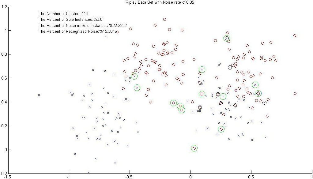$=$ 0.05) on Ripley dataset polluted by %5 class-label noise. Blue X indicates samples from Class 1 and red circles indicate samples from Class 2. The detected sole samples were marked by green circles and the induced labelled noisy samples were marked by black circles.

4.1 Noise filtering using K-means clustering

Figure 5 depicts how the sole samples are detected by the cluster-based filtering method on the Ripley dataset, where %20 class-label noises are induced. As seen in Tables 2 and 3, the achieved results on Adaboost reveal that applying this filtering method leads to a higher accuracy compared to the state that no filtering stage is applied.

Table 2
Noise detection measures using the proposed clustering-based method. For each dataset, the mean value of the calculated measures over 100 randomly-selected test subsets (except for Splice, Image and raw-EEG datasets that have 40 subsets) is reported

		Noise rate $=$ %5		Noise rate $=$ %10		Noise rate $=$ %20
Dataset	Num. clusters	% of sole samples	Noise density	% of sole samples	Noise density	% of sole samples	Noisedensity
Banana	40	0.2%	64.0%	0.2%	74.0%	0.1%	81.0%
Breast	79.4	18.4%	20.0%	18.6%	29.0%	18.2%	37.0%
Diabetis	47	3.3%	22.0%	2.7%	25.0%	2.5%	39.0%
FlareSolar	5.1	0.0%	100%	0.0%	100%	0.0%	0.0%
German	70	4.7%	20.0%	4.4%	33.0%	3.8%	42.0%
Heart	17	4.5%	31.0%	3.6%	52.0%	3.5%	57.0%
Image	21.8	0.2%	100%	0.1%	80.0%	0.1%	83.0%
Ringnorm	40	0.1%	62.0%	0.1%	80.0%	0.2%	85.0%
Splice	973	0.0%	100%	0.0%	63.0%	0.1%	83.0%
Thyroid	14	5.6%	66.0%	5.2%	87.0%	4.1%	74.0%
Titanic	4.2	0.0%	33.0%	0.0%	0.0%	0.0%	0.0%
Two norm	40	0.2%	75.0%	0.2%	89.0%	0.1%	85.0%
Waveform	40	0.2%	69.0%	0.2%	18.0%	0.2%	91.0%
Real EEG	136	3.2%	97.2%	4.4%	96.9%	5.3%	94.1%

Table 3

Error rate of Adaboost (AB) by employing the proposed clustering-based filtering is shown here. For each dataset, the mean values of test error over 100 randomly-selected subsets (except for Splice, Image and raw-EEG datasets that have 40 subsets) are reported for both standard Adaboost and the proposed algorithm (ClustAB). The test error of the proposed algorithm is bolded when it is lower than that of standard Adaboost. HR stands for Hunting Rate and it is calculated by averaging the percentage of hunted noises over all test subsets

Dataset	AB error	ClustAB error	HR	AB error	ClustAB error	HR	AB error	ClustAB error	HR
	Noise rate $=$ %5			Noise rate $=$ %10			Noise rate $=$ %20
Banana	30.1%	29.8%	2.8%	29.6%	29.5%	1.7%	34.0%	33.9%	0.6%
Breast	29.6%	29.3%	73.8%	29.3%	30.1%	53.9%	33.0%	32.1%	33.6%
Diabetis	25.6%	25.6%	14.5%	26.1%	26.5%	6.8%	29.4%	28.9%	4.9%
FlareSolar	34.1%	34.4%	0.5%	36.1%	34.7%	0.3%	35.7%	35.7%	0.0%
German	24.3%	24.7%	18.8%	25.0%	24.8%	14.6%	28.2%	28.2%	8.0%
Heart	24.0%	23.3%	27.9%	24.5%	25.1%	18.7%	28.2%	27.8%	10.0%
Image	5.0%	4.8%	4.6%	5.7%	5.7%	0.8%	8.6%	8.5%	0.2%
Ringnorm	13.0%	13.2%	1.2%	15.4%	15.4%	1.1%	22.1%	21.9%	0.8%
Splice	10.1%	10.1%	0.3%	12.0%	12.1%	0.2%	16.2%	16.0%	0.3%
Thyroid	10.1%	9.2%	73.9%	13.3%	11.6%	45.2%	17.1%	16.8%	15.3%
Titanic	23.7%	23.7%	0.1%	24.4%	24.4%	0.0%	24.3%	24.3%	0.0%
Two norm	9.3%	6.9%	2.9%	11.9%	10.2%	1.8%	17.6%	16.9%	0.6%
Waveform	15.0%	14.3%	2.7%	7.3%	7.1%	1.8%	21.5%	21.0%	0.8%
Real EEG	29.8%	22.1%	3.1%	34.3%	35.7%	4.3%	39.6%	47.1%	5.1%

In Table 2, it can be observed that for most datasets, the noise density increases as the noise rate increases. This trend is particularly noticeable in the Breast, Diabetes, German, Heart, Thyroid, Two norm, and Real EEG datasets. For example, in the Breast dataset, as the noise rate increases from 5% to 20%, the noise density increases from 20.00% to 37.00%.

However, there are some datasets where the noise density remains constant or decreases as the noise rate increases. For instance, in the FlareSolar and Titanic datasets, the noise density remains constant, regardless of the noise rate. The FlareSolar dataset and the Titanic dataset are both very small in terms of the actual number of instances and most of the training and the test samples were created by replications. Therefore, the number of the clusters, and consequently the number of sole samples, are very small for both datasets. This can explain why the clustering method could not be successful on these dataset for recognizing class label noises.

On Table 3, it is apparent that ClustAB outperformed AdaBoost algorithm on most of the benchmark dataset in particular under higher noise levels. Under %5 noise, ClustAB outperformed AB on 10 out of 14 reported benchmark datasets. Under %10 noise, only on 6 benchmark datasets ClustAB could get better results. Under %20 noise, ClustAB could outperform AB again on 10 out of 14 benchmark datasets.

4.2 Noise filtering using AdaBoost

Figure 6.

Histogram of weights in Breath-Cancer database under the noise rate of %20. Dash lines indicate class-label noises over the dataset. Red line and Green line indicate the position of Mean of the weights and Mean 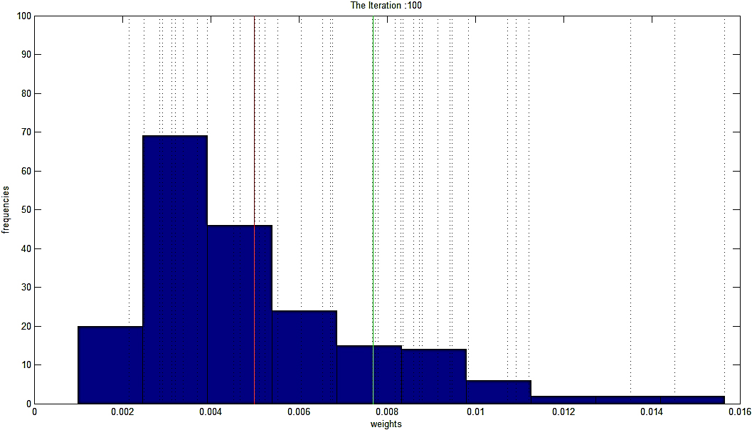$+$ Std, receptively

Figure 6 provides an illustration of weight distribution generated by AdaBoost on the Breath-Cancer dataset, where %20 noisy class-label samples are induced. As it can be seen, the majority of the induced noises (pointed out with Dash-lines) are not necessarily located after the threshold (Mean $+$ Std), nevertheless, the goal here is to hunt the most detrimental noises which are more likely to be among higher weights. The result of the AdaBoost method can be seen in Table 4.

Table 4

Results of AdaBoost (AB) solution. For each dataset, the mean values of test error over 100 randomly-selected subsets (except for Splice, Image and raw-EEG datasets that have 40 subsets) are reported for both standard Adaboost and the proposed algorithm (AB-AB). The test error of the proposed algorithm is bolded when it is lower than that of standard Adaboost. HR stands for Hunting Rate and it is calculated by averaging the percentage of hunted noises over all test subsets

	Noise rate $=$ %5			Noise rate $=$ %10			Noise rate $=$ %20
Dataset	AB error	AB-AB error	HR	AB error	AB-AB error	HR	AB error	AB-AB error	HR
Banana	30.06%	28.32%	14.00%	30.64%	29.70%	18.00%	31.73%	29.88%	13.75%
Breast	30.13%	30.52%	20.00%	29.48%	29.48%	13.00%	34.42%	31.95%	17.50%
Diabetis	25.63%	26.37%	31.30%	27.07%	26.27%	24.68%	27.83%	27.63%	15.96%
FlareSolar	33.95%	34.35%	19.70%	34.18%	34.78%	19.85%	35.18%	34.53%	12.03%
German	23.83%	24.13%	25.14%	25.07%	24.43%	23.71%	27.40%	26.07%	16.43%
Heart	23.70%	21.40%	48.89%	25.40%	23.50%	34.71%	30.30%	28.20%	17.65%
Image	4.88%	5.12%	71.54%	5.75%	5.65%	44.46%	9.04%	8.52%	24.23%
Ringnorm	12.85%	12.98%	49.00%	16.58%	15.98%	34.25%	22.82%	21.80%	20.00%
Splice	10.62%	8.32%	64.00%	11.96%	10.28%	42.30%	16.57%	14.69%	23.00%
Thyroid	10.93%	8.00%	75.71%	13.73%	11.60%	43.57%	17.60%	17.60%	21.43%
Titanic	24.12%	23.92%	25.00%	24.44%	24.61%	16.67%	25.88%	25.71%	16.67%
Two norm	8.62%	6.22%	66.50%	12.60%	9.04%	46.00%	16.70%	14.91%	23.75%
Waveform	15.05%	13.72%	52.50%	17.24%	15.66%	39.75%	22.11%	19.98%	22.50%
Real EEG	29.8%	23.65%	22.88%	34.3%	24.64%	22.75%	39.6%	23.56%	22.90%

Figure 7.

Scatter plots of support vectors’ weights (i.e. Lagrangian coefficients) on the two features of the Ripley dataset under %20 class-label noise. The data points surrounded by red circles indicate class-label noises.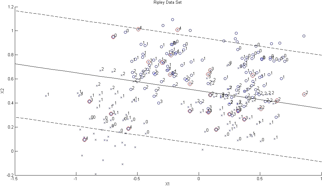

Figure 8.

Histogram of support vectors’ weights under the noise rate of %20. Dash lines indicate class-label noises over the dataset. Red line and Green line indicates the position of Mean of the weights and Mean 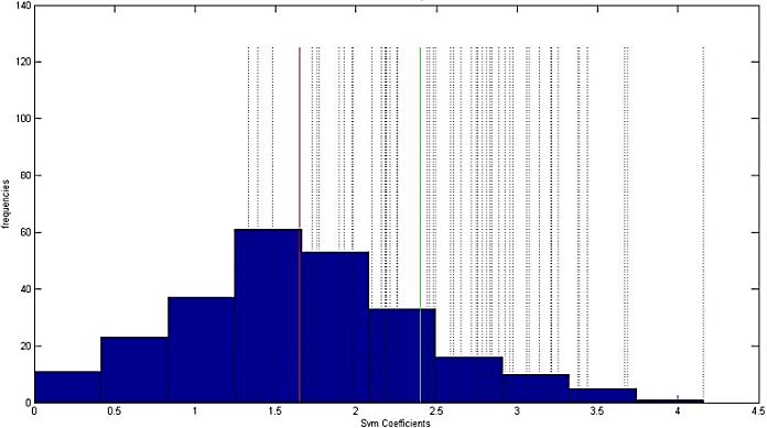$+$ Standard Deviation, receptively.

Table 4 shows that the AdaBoost filtering method outperformed the normal AdaBoost algorithm on most of the benchmark dataset. Under %5 noise, AB-AB outperformed AB on 8 out of 14 reported benchmark datasets. Under %10 noise, this number increases to 11 out 14 and under %20 noise, AB-AB could outperform AB on all of the benchmark datasets except one, the Thyroid dataset where it results is on par with AB.

Considering the hunting rate, under %05 noise, the hunting rate ranges from 14.00% (for Banana dataset) to 75.71% (for Thyroid dataset) with a median of 40.10% for all 14 benchmark datasets. Under %10 noise level, the hunting rate ranges from 13.00% (for Breast dataset) to 46.00% (for Two norm dataset) with a median of 29.47%% for all 14 benchmark datasets. For %20 noise level, the hunting rate ranges from 12.03% (FlareSolar dataset) to 24.23% (Image dataset) with a median of 18.83%.

4.3 Noise filtering using SVM

Figure 7 shows the results of applying the proposed SVM based filtering method to the Ripley dataset under two noise levels of %0 and %20. In this figure, Lagrangian values of all samples are rounded to their nearest integers. It can be observed that the wrongly classified samples have significantly larger Lagrangian values compared to the correctly classified ones (located near to the boundary). It can be seen that all noises, marked by red circles, gained the largest values except the ones which replaced original mislabelled samples.

Figure 8 shows the histogram of weights assigned to the support vectors. Our threshold, Mean $+$ Std is indicated by the green line. According to the histogram, the density of noises increases by incrementing the support vectors’ weights. Interestingly, %99.4 of noise is located after the mean with some completely clean partitions at the beginning. Another point is that the collapse of frequency occurred early after our threshold, which guarantees keeping the amount of deleted samples low enough to have no pernicious effect on learning. The result of the SVM method can be seen in Tables 5 and 6.

Table 5
Noise detection using the proposed SVM filtering is proposed here. For each dataset, the mean values of the calculated measures over 100 randomly-selected subsets (except for Splice, Image and raw-EEG datasets that have 20 subsets) are reported

	Noise rate $=$ %5			Noise rate $=$ %10			Noise rate $=$ %20
Dataset	Deletion rate	Noise density	Hunting rate	Deletion rate	Noise density	Hunting rate	Deletion rate	Noise density	Hunting rate
Banana	16.9%	7.7%	23.5%	16.2%	16.4%	25.5%	18.9%	25.3%	22.9%
Breast	18.5%	17.3%	64.0%	18.9%	31.3%	58.5%	18.9%	49.7%	46.5%
Diabetis	17.6%	19.0%	68.3%	17.7%	35.9%	63.4%	17.4%	58.1%	50.4%
FlareSolar	16.8%	13.4%	45.2%	17.5%	25.1%	39.7%	11.3%	50.4%	25.9%
German	16.9%	18.2%	61.4%	17.2%	34.5%	59.4%	16.6%	57.2%	47.6%
Heart	15.5%	26.9%	77.8%	16.6%	41.2%	68.2%	17.5%	69.9%	61.2%
Image	15.2%	25.8%	78.5%	15.9%	43.2%	68.6%	17.1%	66.4%	56.7%
Ringnorm	14.8%	17.9%	53.0%	14.8%	34.8%	51.5%	14.8%	51.7%	38.4%
Splice	16.3%	24.4%	79.2%	16.2%	44.0%	71.2%	16.5%	68.0%	56.3%
Thyroid	14.6%	31.9%	92.9%	16.0%	51.7%	81.4%	20.0%	74.8%	74.3%
Titanic	22.9%	16.4%	70.0%	22.9%	30.5%	68.7%	25.3%	49.1%	62.0%
Two norm	11.9%	41.2%	97.5%	12.4%	76.1%	94.3%	17.6%	94.1%	82.5%
Waveform	15.1%	27.0%	80.5%	14.6%	47.5%	69.3%	14.6%	72.7%	52.9%
Real-EEG	24.4%	5.2%	37.7%	26.7%	10.8%	43.4%	33.8%	20.2%	51.0%

Table 6

Results of the SVM solution (SVM-AB). For each dataset, the mean values of test error over 100 randomly-selected subsets (except for Splice, Image and raw-EEG datasets that have 40 subsets) were reported for both standard AdaBoost and the proposed algorithm. The test error of the proposed algorithm is bolded when it is lower than that of the standard AB algorithm. HR stands for Hunting Rate and it is calculated by averaging the percentage of hunted noises over all test subsets

	Noise rate $=$ %5			Noise rate $=$ %10			Noise rate $=$ %20
Dataset	AB error	SVM-AB error	HR	AB error	AB-AB error	HR	AB error	SVM-AB error	HR
Banana	29.7%	30.2%	23.5%	31.0%	29.5%	25.5%	31.5%	26.6%	22.9%
Breast	30.1%	28.6%	64.0%	33.1%	32.5%	58.5%	34.2%	28.6%	46.5%
Diabetis	25.9%	25.3%	68.3%	27.2%	26.3%	63.4%	28.7%	27.7%	50.4%
FlareSolar	33.9%	34.3%	45.2%	34.6%	34.3%	39.7%	35.2%	33.0%	25.9%
German	24.7%	24.0%	61.4%	25.1%	25.0%	59.4%	27.7%	23.0%	47.6%
Heart	23.3%	20.0%	77.8%	24.8%	20.0%	68.2%	29.0%	32.0%	61.2%
Image	4.8%	4.1%	78.5%	5.9%	5.9%	68.6%	8.3%	11.0%	56.7%
Ringnorm	12.8%	14.7%	53.0%	15.4%	17.8%	51.5%	22.1%	20.4%	38.4%
Splice	10.6%	10.2%	79.2%	11.3%	10.9%	71.2%	15.7%	14.8%	56.3%
Thyroid	10.9%	14.7%	92.9%	12.9%	20.0%	81.4%	19.7%	16.0%	74.3%
Titanic	23.6%	22.7%	70.0%	23.3%	21.4%	68.7%	24.7%	21.4%	62.0%
Two norm	8.6%	8.2%	97.5%	12.1%	11.3%	94.3%	17.3%	18.2%	82.5%
Waveform	15.9%	16.1%	80.5%	17.2%	17.5%	69.3%	22.8%	21.4%	52.9%
Real EEG	29.8%	31.3%	37.7%	34.3%	30.0%	43.4%	39.6%	38.3%	51.0%

Table 7

Summary of the average improvement made by the employed filtering methods over all randomly-selected subsets across the benchmark datasets

Measure	Filtering method	Noise rate
		%5	%10	%20
% of detected noise (mean $\pm$ standard deviation)	Clustering	17.02 $\pm$ 25.5	11.3 $\pm$ 17.3	5.8 $\pm$ 9.3
	AdaBoost	43.33 $\pm$ 21.0	30.84 $\pm$ 11.5	18.84 $\pm$ 3.8
	SVM	68.6 $\pm$ 19.1	63.1 $\pm$ 21.0	52.1 $\pm$ 21.0
Number of the data sets with improved AB accuracy	Clustering	9	6	10
(out of 13)	AdaBoost	7	10	12
	SVM	8	9	10

Table 5 shows that under %05 noise, the hunting rate ranges from 23.5% (for Banana dataset) to 97.5% (for Two norm dataset) with a median of 69.15% for all 14 benchmark datasets. Under %10 noise level, the hunting rate ranges from 25.50% (for Banana dataset) to 94.30% (for Two-norm dataset) with a median of 65.8% for all 14 benchmark datasets. For %20 noise level, the hunting rate ranges from 22.90% (for Banana dataset) to 82.50% (for Two-norm dataset) with a median of 52.90%. Therefore, the SVM method provides the most stable results across all of the proposed filtering methods with always performing worse on the Banana dataset and performing best on (despite being better than the Two-norm dataset. It should be noted that even the hunting rate achieved on the Banada dataset here is better than AdaBoost and Clustering method by a large margin.

Table 6 shows the effect of noise pruning with the SVM method on the performance of the AdaBoost algorithm. As it can be seen, the SVM-AB method outperformed the simple AB method on 8, 10 and 11 datasets out of the 14 benchmarks under %5, %10 and %20 noise level, respectively.

4.4 Comparing the methods

Results of the proposed filtering methods, as a pre-processing stage for Adaboost, are demonstrated in Table 7. The first observation is that the hunting rates of all three algorithms decline as the noise level increases. However, by observing the enhancement of AdaBoost accuracy, the effectiveness of the proposed schemes to hunt the most detrimental noises, under different levels of noise, is empirically proved. The results show that SVM-filtering outperforms the other two methods in terms of higher hunting rate under various noise intensities. Nonetheless, in terms of improving the AdaBoost performance, as might be expected, the AdaBoost-filtering method holds the highest rank. Although the clustering method does not outperform the other counterparts, it is the winner in terms of affecting just less than 5% of data averagely, with one exception of the Breast-Cancer dataset (Table 2). Considering such a minimal effect, the ability of the clustering method on improving the AdaBoost performance over six to ten datasets is of value.

The hunting rate of the SVM filtering was also not largely affected as the noise level increases compared to the other filtering methods. The good match found between Adaboost and SVM is supported by previous studies [35]. Ratsch et al. reported that the decision line constructed by AdaBoost is similar to the one constructed by SVMs and all support vectors also lie within the step part of the margin distribution for AdaBoost.

5. Conclusion and future work

In this article, three preprocessing methods were introduced for identifying unconfident and noisy samples. To show their effectiveness, they are applied to improve the performance of the AdaBoost classifier, which is famous as a noise sensitive classifier. According to our results, the best presented solution is SVM filtering that employs Lagrangian variables for finding noisy samples. This method shows its strength more and more as the level of noisy data increases from zero to %20 induced noisy samples. The SVM filtering succeeded to hunt more than half of the induced class-label noises as well as to improve the test accuracy over the ten benchmark datasets.

One of our future outlines is extending the SVM filtering method to non-linear kernels. Exploiting the potentials of Lagrangian values in nonlinear kernels can be helpful for developing a more sophisticated noise pruning algorithm. Another idea is to investigate the effect of combining the results of the presented methods for improving the hunting rate. For instance, concentrating on samples found suspected by both AdaBoost and SVM filtering might lead to a better performance in determining class-label noises.

Footnotes

Acknowledgments

No funds, grants, or other support was received.

Conflict of interest

The authors have no competing interests to declare that are relevant to the content of this article.

Data availability statement

All data generated or analysed during this study are included in this published article and its supplementary information files except the EEG dataset which is not publicly available due privacy concerns but are available from the corresponding author on reasonable request.

References

Afshar

Boostani

Sanei

, A combinatorial deep learning structure for precise depth of anesthesia estimation from EEG signals, IEEE Journal of Biomedical and Health Informatics 25(9) (2021), 3408–3415.

Alimardani

Boostani

Taghavi

, Classification of BMD and schizophrenic patients using geometrical analysis of their EEG signal covariance matrices, in: 38th International Conference on Telecommunications and Signal Processing (TSP), Prague, 2015.

Alimardani

Boostani

Blankertz

, Presenting a spatial-geometric EEG feature to classify BMD and schizophrenic patients, International Journal of Advances in Telecommunications Electrotechnics Signals and Systems 5(2) (2016), 79–85.

Alimardani

Boostani

Blankertz

, Weighted spatial based geometric scheme as an efficient algorithm for analyzing single-trial EEGS to improve cue-based BCI classification, Neural Networks 92 (2017), 69–76.

Alimardani

Boostani

, DB-FFR: A modified feature selection algorithm to improve discrimination rate between bipolar mood disorder (BMD) and schizophrenic patients, Iranian Journal of Science and Technology, Transactions of Electrical Engineering 42 (2018), 251–260.

Alimardani

Cho

J.H.

Boostani

Hwang

H.J.

, Classification of bipolar disorder and schizophrenia using steady-state visual evoked potential based features, IEEE Access 6 (2018), 40379–40388.

Angelova

Abu-Mostafa

Perona

, Pruning Training Sets for Learning of Object Categories, in: Proc. IEEE Conf. on Computer Vision and Pattern Recognition, 2005.

Benoît

Ata

, A Comprehensive Introduction to Label Noise. proceedings European Symposium on Artificial Neural Networks, Computational Intelligence and Machine Learning, Bruges (Belgium), 2014, 23–25.

Bostanian

Boostani

Sabeti

Mohammadi

, ORBoost: An Orthogonal AdaBoost, Intelligent Data Analysis 26(3) (2022), 805–818.

10.

Catac

F.O.

, Robust Ensemble Classifier Combination Based on Noise Removal with One-Class SVM, in: 22th International Conference on Neural Information Processing (ICONIP-2015), Istanbul (Turkey), 2015, pp. 10–17.

11.

Chiu

S.L.

, Fuzzy model identification based on cluster estimation, Journal of Intelligent and Fuzzy Systems 2 (1994), 267–278.

12.

Dastgheib

Pouya

O.R.

Lithgow

Moussavi

, Comparison of a new ad-hoc classification method with the ensemble classifiers for the diagnosis of Meniere’s disease using EVestG signals, in: 29’th IEEE Canadian Conference on Electrical and Computer Engineering, Vancouver, Canada, 2016.

13.

Deypir

Alizadeh

Zoughi

Boostani

, Boosting a multi-linear classifier with application to visual lip reading, Expert Systems with Applications 38(1) (2011), 941–948.

14.

Fattahi

Nasihatkon

Boostani

, A general framework to estimate spatial and spatio-spectral filters for EEG signal classification, Neurocomputing 119 (2013), 165–174.

15.

Freund

, A more robust boosting algorithm, arXiv:0905.2138v1, 2009.

16.

Freund

Schapire

, A decision-theoretic generalization of on-line learning and an application to boosting, Journal of Computer and System Sciences, 1997, 119–139.

17.

Friedman

Hastie

Tibshirani

, Additive logistic regression: A statistical view of boosting with discussions, Ann Stat 28(2) (2000), 337–407.

18.

G. Raetsch’s Benchmark Datasets, (n.d.), Retrieved from http://theoval.cmp.uea.ac.uk/∼gcc/matlab/default.html#benchmarks.

19.

Haussler

Warmuth

, The probably approximately correct (PAC) and other learning models, Foundations of Knowledge Acquisition, 1993, 291–312.

20.

Hickey

, Noise modelling and evaluating learning from examples, Artif. Intell 82(1–2) (1996), 157–179.

21.

Jiang

, Some theoretical aspects of boosting in the presence of noisy data, in: Proc. 18th Int. Conf. Machine Learning, Williamstown, MA, 2001, pp. 234–241.

22.

Ken

, Data quality and systems theory, Commun. ACM 41(2) (1998), 66–71.

23.

Keshani

Azimifar

Tajeripour

Boostani

, Lung nodule segmentation and recognition using SVM classifier and active contour modeling: A complete intelligent system, Computers in Biology and Medicine 43(4) (2013), 287–300.

24.

Koshiba

Abe

, Comparison of L1 and L2 SVMs, in: Proceedings of the International Joint Conference on Neural Networks, 2003.

25.

Maller

Lithgow

Gurvich

Haghgooie

Pouya

O.R.

Fitzgerald

Kulkarni

, Separating mental disorders using vestibular field potentials, Archives of Neuroscience 2(2) (2014), e19257.

26.

Malossini

Blanzieri

, Detecting potential labeling errors in microarrays by data perturbation, Bioinformatics 22(17) (2006), 2114–2121.

27.

Melville

Shah

Mihalkova

Mooney

R.J.

, Experiments on Ensembles with Missing and Noisy Data, in: ICML ’04 Proceedings of the Twenty-First International Conference on Machine Learning, 2004, pp. 293–302.

28.

Merler

Caprile

Furlanello

, Bias-variance control via hard points shaving, International Journal of Pattern Recognition and Artificial Intelligence, 2004.

29.

Merler

Caprile

Furlanello

, Bias-variance control via hard points shaving, International Journal of Pattern Recognition and Artificial Intelligence, 2004.

30.

Moayedi

Azimifar

Boostani

Katebi

S.D.

, Contourlet-based mammography mass classification using the SVM family, Computers in Biology and Medicine 40(4) (2010), 373–383.

31.

Muhlenbach

Lallich

Zighed

D.A.

, Identifying and handling mislabeled instances, 22(1) (2004).

32.

Nezam

Boostani

Abootalebi

Rastegar

, A novel classification strategy to distinguish five levels of pain using the EEG signal features, IEEE Transactions on Affective Computing 12(1) (2021), 131–140.

33.

Parvinnia

Sabeti

Jahromi

M.Z.

Boostani

, Classification of EEG Signals using adaptive weighted distance nearest neighbor algorithm, Journal of King Saud University-Computer and Information Sciences 26(1) (2014), 1–6.

34.

Pouya

O.R.

, A new Margin-based AdaBoost Algorithm: Even more robust than RobustBoost to class-label noise, in: 2016 IEEE Canadian Conference on Electrical and Computer Engineering (CCECE), Vancouver, Canada: IEEE, 2016, pp. 1–5.

35.

Ratsch

Onoda

Muller

, An asymptotic analysis of AdaBoost in the binary classification case, in: Proceeding of the International Conference on Artificial Neural Networks, 1998.

36.

Ratsch

Onoda

Muller

, Soft margins for AdaBoost, Machine learning, 2001, 287–320.

37.

Redman

, The impact of poor data quality on the typical enterprise, Commun. ACM 2(2) (1998), 79–82.

38.

Sabeti

Katebi

S.D.

Boostani

, Entropy and complexity measures for EEG signal classification of schizophrenic and control participants, Artificial Intelligence in Medicine 47(3) (2009), 263–274.

39.

Sabeti

Boostani

Katebi

S.D.

Price

G.W.

, Selection of relevant features for EEG signal classification of schizophrenic patients, Biomedical Signal Processing and Control 2(2) (2007), 122–134.

40.

Sabeti

Katebi

S.D.

Boostani

Price

G.W.

, A new approach for EEG signal classification of schizophrenic and control participants, Expert Systems with Applications 38(3) (2011), 2063–2071.

41.

Sabeti

Boostani

Zoughi

, Using genetic programming to select the informative EEG-based features to distinguish schizophrenic patients, Neural Network World 22(1) (2012), 3–20.

42.

SáEz

Luengo

Herrera

, Predicting noise filtering efficacy with data complexity measures for nearest neighbor classification, Pattern Recognition 46(1) (2013), 355–364.

43.

Schapire

Freund

Bartlett

Lee

, Boosting the margin: A new explanation for the effectiveness of voting methods, Ann Stat 26(5) (1998), 1651–1686.

44.

Sharifinia

Boostani

, Instance-based cost-sensitive boosting, International Journal of Pattern Recognition and Artificial Intelligence 34(3) (2020), 2050002.

45.

Smyth

Fayyad

Burl

Perona

Baldi

, Inferring ground truth from subjective labelling of venus images, Advances in Neural Information Processing Systems 7, Denver, CO., 1994, 1085–1092.

46.

Taghavi

Boostani

Sabeti

Taghavi

S.M.A.

, Usefulness of approximate entropy in the diagnosis of schizophrenia, Iranian Journal of Psychiatry and Behavioral Sciences 5(2) (2011), 62–70.

47.

Taheri

Boostani

, Novel Auxiliary Techniques in Clustering, World Congress on Engineering, London (UK), 2007, 243–248.

48.

Vezhnevets

Barinova

, Avoiding boosting overfitting by removing confusing samples, in: European Conference on Machine Learning, Springer, Berlin, Heidelberg, 2007, September, pp. 430–441.

Enhancing Adaboost performance in the presence of class-label noise: A comparative study on EEG-based classification of schizophrenic patients and benchmark datasets

Abstract

Keywords

1. Introduction

2. Method

2.1 Adaboost

2.2.1 Combination of K-means & KNN

Table 1 Description of the benchmark datasets

3.3 Higuchi fractal dimension

3.5 Noise density

3.6 Hunting rate

4. Experimental results

Table 2 Noise detection measures using the proposed clustering-based method. For each dataset, the mean value of the calculated measures over 100 randomly-selected test subsets (except for Splice, Image and raw-EEG datasets that have 40 subsets) is reported

Table 5 Noise detection using the proposed SVM filtering is proposed here. For each dataset, the mean values of the calculated measures over 100 randomly-selected subsets (except for Splice, Image and raw-EEG datasets that have 20 subsets) are reported

5. Conclusion and future work

Footnotes

Acknowledgments

Conflict of interest

Data availability statement

References

Table 1
Description of the benchmark datasets

Table 2
Noise detection measures using the proposed clustering-based method. For each dataset, the mean value of the calculated measures over 100 randomly-selected test subsets (except for Splice, Image and raw-EEG datasets that have 40 subsets) is reported

Table 5
Noise detection using the proposed SVM filtering is proposed here. For each dataset, the mean values of the calculated measures over 100 randomly-selected subsets (except for Splice, Image and raw-EEG datasets that have 20 subsets) are reported