
Abstract
Evaluating and comparing models with respect to their predictive performance is a cornerstone of Bayesian statistics. Two related and important techniques are leave-one-out cross-validation and stacking. Both quantify and set in relation the ability to predict unseen observational units from the same data-generating process for a set of models. Recent advancements in software development—in particular, the Stan modeling framework—have made it possible to apply these techniques easily to a wide range of models. However, in more complex models, such as the widely applied classes of hierarchical models and mixture models, the choice of observational unit is not trivial and can result in the need for numerical integration, in particular in non-normal models. We present a case study of Bayesian mixture item response models for cross-classified multirater data, where the most parsimonious choice of observational unit required two-dimensional integration. We show that implementing a numerical quadrature scheme directly within the Stan model code, which is available as Supplemental Data, allows for efficient and accurate estimation of predictive performance.
Keywords
Bayesian predictive model evaluation is increasingly popular in the social and behavioral sciences, especially for evaluating and comparing complex statistical (e.g., psychometric) models. The leave-one-out cross-validation (LOO-CV; Bernardo & Smith, 2004; Geisser & Eddy, 1979; Vehtari & Ojanen, 2012; Vehtari et al., 2017) index can be viewed as a generalization of the Akaike information criterion (AIC; Akaike, 1998; Stone, 1977), providing an estimation of out-of-sample predictive accuracy. In contrast to the AIC, it quantifies the uncertainty contained in the assessment of predictive accuracy and takes into account all the information contained in the Bayesian analysis. Moreover, it provides additional diagnostics, such as stability coefficients and an effective number of parameters, informing researchers of the reliability of results as well as potentially misbehaved observational units and the degree of overfitting, respectively. For this reason, the usage of LOO-CV is preferred to traditional information criteria such as AIC or, similarly, the Bayesian information criterion (BIC; Schwarz, 1978), in a fully Bayesian analysis (Gelman et al., 2014; McElreath, 2020; Weakliem, 1999).
LOO-CV amounts to calculating the sum of the log predictive densities for each observational unit, conditional on all other units (Vehtari & Ojanen, 2012). In Bayesian analysis, it is typically implemented using efficient approximations, such as Pareto-Smoothed Importance Sampling (PSIS-LOO; Vehtari et al., 2017), which avoids the need to re-fit the model multiple times, making it computationally efficient. Stacking weights (or model averaging weights) can be used alongside PSIS-LOO (Yao et al., 2018). They can improve predictive performance by optimally combining multiple models, thereby capturing a broader range of uncertainty and mitigating the impact of any single model’s misspecification (Piironen & Vehtari, 2017).
How observational units are defined is a choice left to the practitioner. Although more general forms of LOO-CV have been introduced (see, e.g., Bürkner et al., 2020, 2021), the usual conceptualization of LOO-CV and its implementation via PSIS requires observational units to be exchangeable such that the likelihood can be factorized (Vehtari et al., 2017; Yao et al., 2018). This structure is required, for example, by the frequently used R (R Core Team, 2021) package loo (Vehtari, Gabry, et al., 2022) that is closely associated with the Stan modeling framework (Stan Development Team, 2022).
In simple models, such as linear regression, the only available choice is the singular data points. For hierarchical models, however, each level represents a possible choice of unit (Vehtari & Ojanen, 2012; Vehtari et al., 2017). If, for example, students are nested in classes that are themselves nested in schools, cross-validation can refer to predicting new students from existing classes, new classes with new students from existing schools, or new schools altogether.
An important special case of hierarchical models in psychology is psychometric latent variable models (Hoyle, 2012; Irwing et al., 2018). Typically, they are used to analyze data with respondents giving answers to a set of items, which induces a natural nesting of item answers in persons. These models are used to measure a latent construct, and therefore each person is associated with a person-specific parameter.
When persons are taken as the observational unit, this is problematic for PSIS-LOO (and thus, efficient stacking implementations based on it), because leaving out a person means leaving out the information that is used to estimate this person’s parameter (Gelman et al., 2014). In this case, each observational unit is highly informative for the posterior distribution (Vehtari et al., 2017). Thus, unit-specific parameters must be eliminated to use PSIS-LOO (Millar, 2018)—either analytically, by approximation, or, when such efficient solutions are not available, by numerical integration. In psychometrics, this is the case for ordinal factor models and other models with non-normal likelihoods, such as those based on item response theory (IRT; van der Linden & Hambleton, 1997). These models were developed to analyze responses on items with ordered categories that are common in surveys as well as psychological testing.
One reason to define the person as the observational unit in a psychometric latent variable model, instead of the individual item responses are theoretical considerations. Specifically, leaving out individual responses implies evaluating the model’s ability to predict new responses by the same persons on the same items, whereas leaving out persons (i.e., response vectors on the given set of items) estimates the predictive accuracy for new responses by new persons on the same items. The latter is the theoretically more pertinent quantity because researchers are usually interested in evaluating how well a model generalizes to a target population of respondents (Merkle et al., 2019).
Another reason to perform cross-validation on the person level is that in some models, the likelihood cannot be factorized within persons. This is the case for mixture models assuming latent subpopulations of respondents that a model is tasked to infer from the data (De Ayala & Santiago, 2017; von Davier & Rost, 2006). In these models, the probability of a person giving some response on an item depends on class membership, which implies non-exchangeability. Then, only full response vectors representing persons, with class membership parameters marginalized out of the individual likelihood contributions, can be exchangeable.
The problem of marginalizing out unit-specific parameters is exacerbated when multiple levels are nested within the observational unit. This is the case, for example, in multi-rater models (Eid et al., 2025). Here, each target (e.g., teachers) is associated with multiple raters (e.g., students), and the target as well as all raters are equipped with parameters. When each rater is additionally associated with multiple targets, then cross-classified models (Eid et al., 2025; Koch et al., 2016) can be fit, which separate rater-, target-, and interaction effects, which all represent different latent variables. Then, taking either targets or raters as the observational unit implies integrating out their specific parameters as well as interaction effects, resulting in the need for two-dimensional integration.
In this paper, we present a case study of how cross-validation and stacking can be performed for Bayesian cross-classified IRT models containing a mixture distribution assumption for the rater population. The analyzed data are teaching evaluations from our university, and the models were chosen to find and control for student response styles, while also accounting for the ordinal nature of responses as well as the cross-classified data structure to maximize the validity of the evaluation. The models are fit in the Stan modeling language, and we show how two-dimensionally integrating out unit-specific parameters makes it possible to do model evaluation and comparison by means of the loo package.
Predictive Model Evaluation
In this section, we briefly summarize the mathematical basis of PSIS-LOO and stacking to introduce the quantities of interest we calculated in our study. An extensive overview of Bayesian predictive methods is given by Vehtari and Ojanen (2012), and an abridged and more practically oriented version containing recommendations was published by Piironen and Vehtari (2017). More information on and introductions to PSIS-LOO can be found in Gelman et al. (2014) as well as Vehtari et al. (2017), and, for stacking, Yao et al. (2018).
PSIS-LOO
Consider a collection of
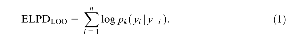
When individual units are predicted conditional on the complete data
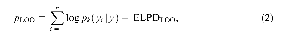
can be calculated. When compared with the actual number of parameters a model has,
Exact LOO-CV requires re-fitting the model

Moreover, for each observation
Stacking
In stacking, LOO-CV is performed with all
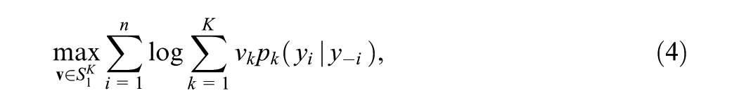
where
Elimination of Unit-Specific Parameters
As discussed in the introduction section, when each observational unit is associated with its own unit-specific parameter(s), they must be eliminated to do PSIS-LOO by means of the loo R package. In certain special cases, this can be done by conditioning on sufficient statistics (Basu, 1977). Generally, however, the likelihood must be marginalized with respect to these parameters (Merkle et al., 2019; Vehtari et al., 2016), that is, they must be integrated out. In this case, the model can be represented in two ways: either based on the conditional likelihood, still containing the nuisance parameters, or on the marginal one (cf. Merkle et al., 2019). Using the marginal likelihood while fitting the model reduces the size of its parameter space and thus stabilizes the MCMC sampling process (Merkle & Rosseel, 2018). However, when marginalization is computationally expensive, it can be faster to integrate out parameters post-hoc, that is, for each draw from the posterior distribution, the likelihood is marginalized with the draw’s remaining parameter values plugged in.
For Gaussian models, closed-form expressions for the integrals might exist (Merkle & Rosseel, 2018) or efficient approximations can be used (Vehtari et al., 2016). For many other important classes of models, neither closed forms nor approximations exist. Then, numerical integration must be performed. Merkle et al. (2019) used adaptive Gaussian quadrature post-hoc to eliminate person parameters in psychometric models in order to do PSIS-LOO. Stan comes with its own integrator function that uses double exponential quadrature as implemented in the Boost C++ library (Agrawal et al., 2017; Takahasi & Mori, 1973). In preliminary tests, we found it to perform more efficiently than adaptive Gaussian quadrature when implemented directly in the generated quantities block of our Stan models, which allowed us to optimize this process by reusing calculations. The code for all models can be found in Supplemental Data (available in the online version of this article).
Analyzing Teaching Evaluation Data
In educational research and evaluation, cross-classified structures arise naturally since students usually attend multiple courses and therefore submit multiple ratings (cf. Pagani & Seghieri, 2002). Figure 1 visualizes the data structure for a minimal teaching evaluation design with four teachers and three students. As can be gathered from this figure, every response vector (i.e., a row in the table) is nested within one rater as well as one target. A set of response vectors pertaining to the same target, however, is not nested within any single rater (indicated by the black rectangle around all response vectors exemplarily for target 2 in Figure 1). On the other hand, a set of response vectors pertaining to the same rater is not nested within any single target (indicated by the dashed rectangles around all response vectors exemplarily for rater 2 in Figure 1). Thus, there are two possible hierarchies—one for raters and the other for targets (NB: targets and raters can also be considered dummy-coded variables on an auxiliary top-level; for details see Skrondal & Rabe-Hesketh, 2004).
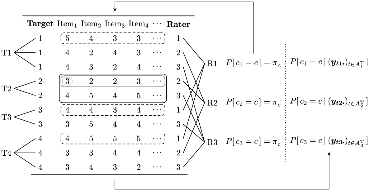
Cross-classified data structure for a minimal teaching evaluation design.
On the right, the updating of class membership probabilities is schematically illustrated for a mixture of raters as was implemented in the present work. Each rater is assigned prior class membership probabilities
While this structure renders classical multilevel models inappropriate, in return, it makes it possible to assess target and rater biases separately. This enables researchers to quantify the interdependency of targets and raters and relate this measure to the variation in target and rater latent traits. Specifically, a high degree of interdependency indicates that responses cannot be well explained by the latent trait of the target (e.g., teaching ability) and is, therefore, detrimental to the validity of the evaluation—which is a controversial subject in the pertinent literature (Kromrey, 1994; Marsh, 1984, 1987; Rindermann, 2001; Wolbring, 2013a, 2013b).
Despite the ubiquity of this complex data structure in teaching evaluation, often rather simplistic statistical tools (e.g., sum scores and multiple regression) are used to analyze these data in practice, not controlling for confounding effects such as measurement error (Ziegler & Weis, 2015). This shows a lack of suitable models and analysis techniques that have been tested and tried and are available to a broad audience. One candidate is cross-classified multilevel models (or crossed random effects models; Goldstein, 1994, 2010). They allow the explicit modeling of the dependencies induced by the data structure and separate target, rater, as well as target–rater interaction effects. Simulation studies show that fitting multilevel models and thus ignoring the cross-classification leads to biased estimates (in particular, inflation of standard errors; Schultze et al., 2015). Multilevel confirmatory factor analysis models have been recommended (Sengewald & Vetterlein, 2015). They allow to explicitly model measurement error and to specify measurement models on multiple levels (see, e.g., Koch et al., 2014, 2015, 2016).
Few publications have unified these two approaches. Koch et al. (2016) provided an extension to cross-classification for multitrait-multimethod designs with continuous observed variables based on the multilevel correlated trait-correlated method minus 1 [CTC(M − 1)] model by Eid et al. (2008). For these types of data, the model allows the explicit modeling of measurement error and cross-classified effects (latent traits), the combination of various types of methods (e.g., self-assessment and multiple rater assessments per target), estimation of convergent and discriminant validity, regression of cross-classified effects on covariates, as well as the calculation of variance coefficients and (un)reliability.
Nevertheless, teaching evaluation is based on Likert scales, and thus models for continuous outcomes are not appropriate (Liddell & Kruschke, 2018). Rather, because the assessment of a latent trait, such as teaching quality, is the main concern, IRT models should be used. Two major families of IRT models are cumulative models on the one hand and adjacent-category models on the other (Bürkner & Vuorre, 2019). They are often related to different assumptions about the underlying response process (see also Andrich, 1995). While the first family is linked to factor analysis and the discretization of an auxiliary latent continuous variable (Takane & de Leeuw, 1987), the second can be related to an assumed decision process (see, e.g., Plieninger & Meiser, 2014). Oftentimes, it is not obvious a priori which class of models is more appropriate to a given application, and a choice is made based on which mathematical properties of either model are more in line with the research goals or, if available, on fit indices (Bürkner & Vuorre, 2019). Therefore, in the present work, we extend the model by Koch et al. (2016) to each of these families’ most prominent representatives: the graded response model (GRM; Samejima, 1969, 1997), respectively, the generalized partial credit model (GPCM; Muraki, 1992, 1997).
Additional complexity in teaching evaluation data comes from students differing qualitatively in their utilization of questionnaires (Bacci & Gnaldi, 2015), which results in differential item functioning. In particular, students may show certain response styles, such as the preference for the upper and lower ends of a scale, known as extreme responding, or the tendency to agree and thus choose positively worded categories in the upper half of the scale, called acquiescence (for an overview, see Van Vaerenbergh & Thomas, 2013). Mixture IRT (Mix-IRT) models (De Ayala & Santiago, 2017; Rost, 1990; von Davier & Rost, 2006) represent a combination of latent class analysis (LCA) and IRT and are one of many approaches appropriate to model this kind of heterogeneity (cf. Henninger & Meiser, 2020). They represent an exploratory approach by assuming that each observational unit (e.g., students; for more details, see the Model Description section) belongs to any of a fixed number of groups (or classes, in the vocabulary of LCA) that do not need to be known beforehand but can be inferred from the data. Advantageously, this implies relaxing the assumptions of unidimensionality (cf. Rijmen & De Boeck, 2005) and local independence. At the same time, Mix-IRT models allow to check for measurement invariance because the latent classes can potentially differ in any of the parameters of the model, such as difficulty parameters or latent variances.
There are various examples of these models being applied to standard multilevel data (Cho & Cohen, 2010; Fox, 2005; Lee et al., 2018; Vermunt, 2008a, 2008b). However, few publications considered Mix-IRT models in the context teaching evaluation (Bacci & Gnaldi, 2015) and especially in conjunction with cross-classified data structures (Jin & Wang, 2017; Kelcey et al., 2014).
To account for all aforementioned intricacies of teaching evaluation data, we integrated these modeling techniques into a unified approach that we call mixture cross-classified item response theory (Mix-CC-IRT) models. In the following, we give their likelihoods after introducing their components.
Model Description
Consider the evaluation of target (i.e., teacher)
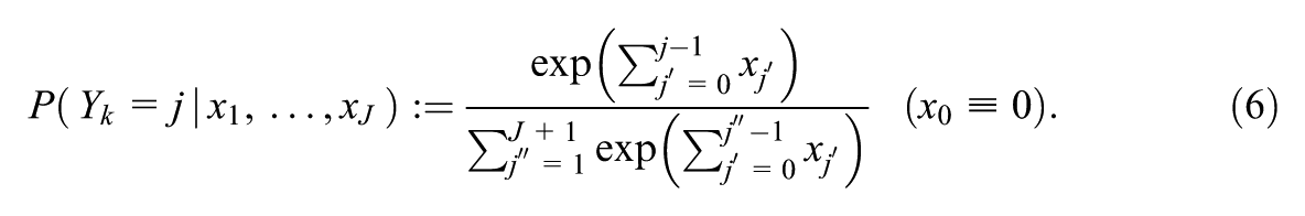
And for the GPCM by
Because the GRM is a cumulative model and probabilities cannot be negative, it needs to hold that
We assume that there are
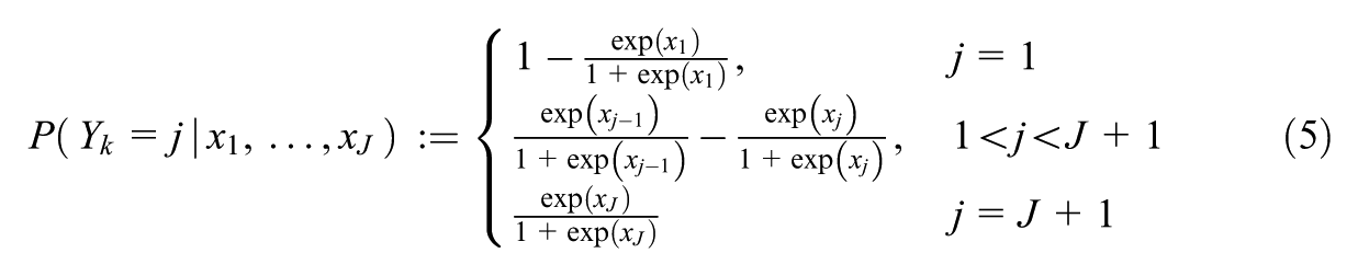
In the present case, for each item

The parameters
Bayesian posterior sampling methods (such as Hamiltonian Monte Carlo as implemented in Stan; Stan Development Team, 2022) can be made more efficient by breaking down parameters into their independent and centered components. Thus, we further split the item parameters into common tendency and deviation parameters. For the thresholds, we set
As scaling parameters, the factor loadings need to be positive. In Stan, this constraint is implemented via a


and
Note that the only elementary parameters to vary across classes are
Collecting all parameters in
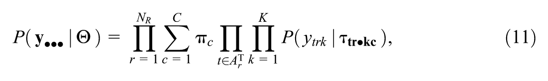
where the sets
For the application of PSIS-LOO and stacking, marginalized likelihood contributions for each rater need to be calculated by approximating the following quantity:
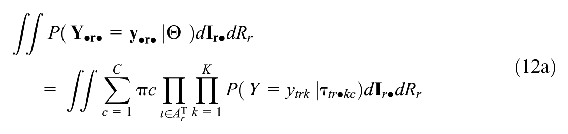
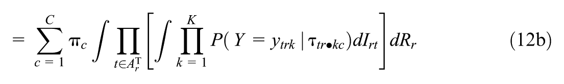
The parameters
Since calculating integrals in each proposed jump of the Markov Chain is very costly, the estimation of the model is based on the conditional, rather than marginalized, likelihood. For this reason, the integral in Equation 12b is evaluated only in the “generated quantities” block of our Stan models. To reduce the number of individual function evaluations, we implemented the double exponential quadrature directly inside the generated quantities block of our Stan models, which allowed us to circumvent needlessly recalculating nonvarying parts of the likelihood (e.g., the sums of item parameters and teacher ability parameters within the composite parameters
Application
We fitted both
Ethical Statement
The data analysis was planned and approved as part of a research project funded by the German Research Foundation (project number 405463675). The data were used with permission from the Friedrich Schiller University Jena under a usage agreement and the analysis fully complied with the ethical guidelines of the German Psychological Society.
Data Availability
The data cannot be shared with third parties for privacy reasons.
Data Preparation
The data preparation process is described in detail in Supplemental Appendix A (available in the online version of this article). It resulted in
Fitting Procedure
For each model, four chains were used with 2,000 warmup and 8,000 sampling iterations per chain. Because Hamiltonian Monte Carlo [HMC] is highly effective no thinning is necessary (except for the Mix-CC-
Prior Specification and Identification of Mixture Parameters
The full prior specification can be found in Table A1 (available in the online version of this article). To achieve a high efficiency of the sampler and a satisfactory convergence of the Markov chains, appropriate reparameterizations (e.g., restricting the use of hyperparameters and soft constraints for parameter decompositions) and distributions with low variances were employed. A full justification for the prior model is given in Supplemental Appendix A (available in the online version of this article).
A known issue in mixture modeling is that latent classes are exchangeable, that is, the posterior distribution is invariant with respect to the permutation of class indices (Frühwirth-Schnatter, 2001). Apart from the post-hoc relabeling of classes (e.g., by means of the label.switching package; Papastamoulis, 2016), this issue can be dealt with by imposing an ordering constraint on any quantity varying across classes in the model. We used the latter technique to identify the latent classes, the details of which are given in Supplemental Appendix A (available in the online version of this article).
Results
Convergence
For all models, no divergent transitions were observed, no iteration reached the maximal treedepth, and the estimated Bayesian fraction of missing information was close to 0.6 for all chains (for more information about these measures, refer to Vehtari et al., 2021, Betancourt, 2018, as well as the Stan users guide, Stan Development Team, 2022). Moreover, all models but the
For the Mix-CC-
Selected Parameters
The focus of this article is on cross-validation and not on the analysis itself, which is why we only report posterior quantities of parameters that can inform the cross-validation results. In particular, it is important to understand how, within one type of model (i.e., either within the GRM or the GPCM), the two- and three-class solutions differ with respect to their predictions. In the following, a circumflex designates a posterior quantity. In the main body of the text, we report posterior means and 90% posterior intervals. Quantities whose Monte Carlo standard errors exceed 0.01 are underlined.
In the Mix-CC-
Overall, items were very easy and overall easiness did not differ between classes when taking into account the 90% posterior intervals. Indeed,
On the other hand, the sample variance of the centered thresholds (note the sum-to-zero constraint)
In the
In the
In the
Predictive Model Evaluation
Leave-One-Out Cross-Validation
First, we checked Pareto-
Leave-One-Out Cross-Validation Results
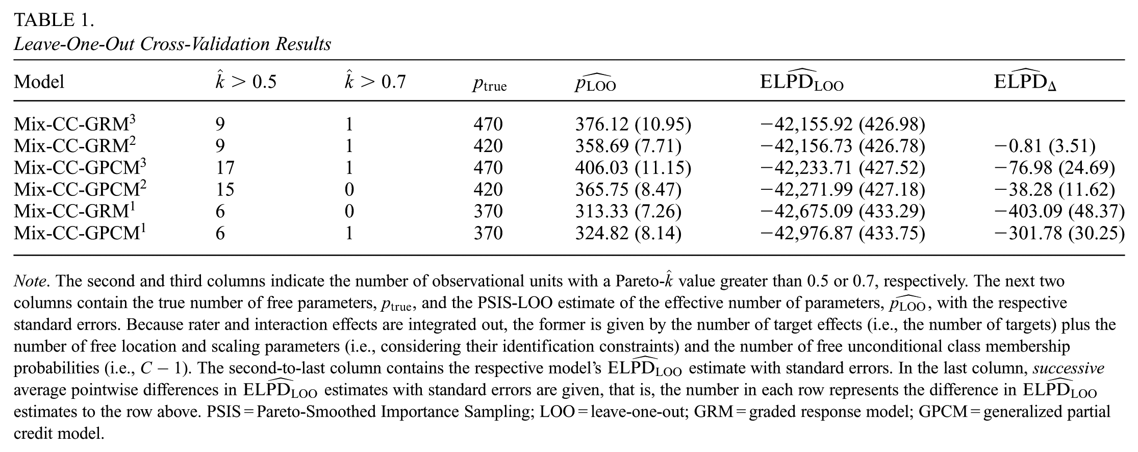
Note. The second and third columns indicate the number of observational units with a Pareto-
As another diagnostic, the effective number of parameters estimated by PSIS-LOO,
Since the statistical quantities
As Table 1 suggests, the Mix-CC-GRM3 dominates the other models in terms of
On the other hand, the Mix-CC-GPCM3 had a higher predictive accuracy than the Mix-CC-GPCM2, even considering the standard error of the differences. For the remaining one-class models, the successive differences in
Stacking
We performed stacking in three different ways. First, we stacked all models together, resulting in six weights that altogether sum up to 1. Second, we stacked the models by class, that is, we only included models with the same number of classes in the stacking procedure, resulting in three pairs of weights. Third, we stacked the one-, two-, and three-class solutions of each type of IRT model, resulting in two weight triples.
The results are given in Table 2. They reflect, roughly, those of the PSIS-LOO procedure. Whereas the Mix-CC-GRM2 and Mix-CC-GRM3 share considerable parts of the prediction weight in Tables 2a and 2c, the Mix-CC-GPCM3 outperforms the Mix-CC-GPCM2 in both stacks. Interestingly, the one-class solutions take up around 10% of the weight, both in Table 2a, when adding the weights of both one-class solutions, as well as in the stacking by model in Table 2c. This indicates that there are observational units that are either not adequately predicted by the higher-class solutions or, conversely, that are as accurately predicted by models with only one class.
Stacking Weights
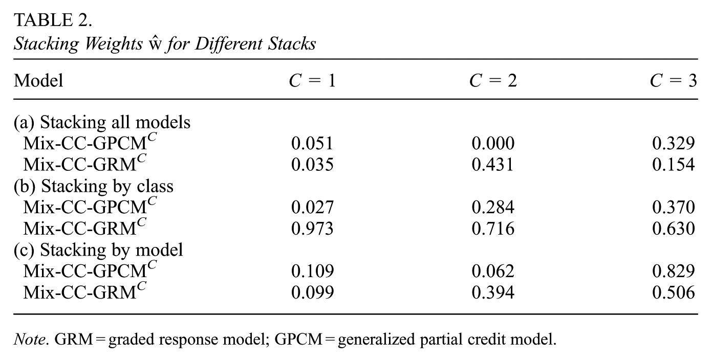
Note. GRM = graded response model; GPCM = generalized partial credit model.
Discussion
In this study, we showed how to perform predictive model evaluation using PSIS-LOO and stacking in mixture cross-classified IRT models. These procedures were made possible by integrating out rater and interaction parameters. Our implementation of the models, as well as the double exponential quadrature, led to satisfactory results. The corresponding Stan code is part of the Supplemental Data (available in the online version of this article) and can be extended and adapted to other applications.
The advantages of predictive model evaluation are particularly apparent in the context of our application because of the high number of degrees of freedom in the modeling process. First, specifying a higher number of latent classes can make the models more flexible and thus improve the fit to the data, which, at the same time, bears the risk of overfitting. The information provided by LOO-CV and stacking can help to find redundancies and identify overparameterizations. In our case, this meant comparing the effective and true number of parameters as well as considering the stacking weights for the one-class models.
Second, adjacent-category and cumulative models can be employed for the same purpose, and they share many features. It is often assumed that the choice between adjacent-category vs. cumulative models is one of researcher preferences or interpretability (Andrich, 1995). The present results paint a more nuanced picture. The magnitude of the difference in predictive power depends on how many classes are used. In the one-class solutions, the Mix-CC-
In addition, this case study shows how stacking can provide valuable information beyond raw prediction scores. When stacked only against the Mix-CC-GRM1, the Mix-CC-GPCM1 is assigned negligible weight, reinforcing the evidence for a true benefit in prediction when choosing the former over the latter. Considering either the class-wise stacking results or when all models are stacked together, the combined weights of both types of models are of almost equal magnitude, which indicates that they performed similarly for a sizeable portion of observational units. Nevertheless, from the distribution of weights, it can also be concluded that, while the Mix-CC-GPCM3 might perform comparably to the Mix-CC-GRM2, it requires an additional class to do so.
The previous considerations make it clear that predictive model evaluation can yield unique insight beyond conventional fit indices. They provide diagnostic information concerning not only the predictive criteria but also with respect to the stability of estimation, as well as conspicuous observational units. Next, the
This has important practical implications for educational researchers. First, it enables the systematic testing and comparison not only of measurement invariance assumptions but also of fundamentally different classes of models that assume distinct underlying measurement processes. For example, in an educational assessment context, a researcher might find that a model including response-style effects outperforms one without such effects in predictive accuracy, yet both yield similar ability estimates. This result would indicate the presence of response styles while also supporting the unbiasedness of ability estimates. Conversely, two models assuming different response processes might share predictive weight in the stacking procedure but produce conflicting ability estimates, implying noninvariance in how the ability parameter should be interpreted.
Second, it is straightforward to extend these models by including covariates to predict teaching ability. Estimating the degree of parameter pooling that leads to optimal predictive performance can provide valuable information for policymakers, helping to distinguish, for example, between school-specific and district-level dependencies in teaching effectiveness.
Lastly, predictive model selection can guide future research by revealing whether theoretical assumptions about data structures lead to optimal predictions. Discrepancies may point to problems in model formulation or the interpretation of parameters. A promising direction for future work lies in exploring why certain observational units are better predicted by particular models. The diagnostic information provided by LOO-CV offers a first line of investigation: Pareto-
Hierarchical stacking (Yao et al., 2022) offers another, more advanced, approach: unit-level log-likelihoods from multiple models are analyzed jointly within a hierarchical mixture framework, possibly with covariates. This allows each unit to receive its own set of model weights, and the resulting distribution of weights can illuminate interactions between model structure and unit characteristics.
Overall, a key advantage of cross-validation and stacking is that they allow inferences that extend beyond the mere selection of a single “best” model from a candidate set. As demonstrated in this case study, these approaches can be successfully applied even to complex, non-normal models with nested random effects using the standard Bayesian modeling toolkit.
Supplemental Material
sj-pdf-1-jeb-10.3102_10769986261422706 – Supplemental material for Predictive Model Evaluation in Bayesian Mixture and Hierarchical Models for Ordinal Data: A Teaching Evaluation Case Study
Supplemental material, sj-pdf-1-jeb-10.3102_10769986261422706 for Predictive Model Evaluation in Bayesian Mixture and Hierarchical Models for Ordinal Data: A Teaching Evaluation Case Study by R. Maximilian Bee and Tobias Koch in Journal of Educational and Behavioral Statistics
Supplemental Material
sj-zip-2-jeb-10.3102_10769986261422706 – Supplemental material for Predictive Model Evaluation in Bayesian Mixture and Hierarchical Models for Ordinal Data: A Teaching Evaluation Case Study
Supplemental material, sj-zip-2-jeb-10.3102_10769986261422706 for Predictive Model Evaluation in Bayesian Mixture and Hierarchical Models for Ordinal Data: A Teaching Evaluation Case Study by R. Maximilian Bee and Tobias Koch in Journal of Educational and Behavioral Statistics
Footnotes
Declaration of Conflicting Interests
The authors declared no potential conflicts of interest with respect to the research, authorship, and/or publication of this article.
Funding
The authors disclosed receipt of the following financial support for the research, authorship, and/or publication of this article: The work was funded by the German Research Foundation (DFG project number: KO 4770/2-1).
Authors
RICHARD MAXIMILIAN BEE is a PhD student at the Psychological Methods division, Friedrich-Schiller-Universität Jena, Am Steiger 3, 07743 Jena, email:
TOBIAS KOCH is full professor for Psychological Methods at the Friedrich-Schiller-Universität Jena, Am Steiger 3, 07743 Jena, email:
References
Supplementary Material
Please find the following supplemental material available below.
For Open Access articles published under a Creative Commons License, all supplemental material carries the same license as the article it is associated with.
For non-Open Access articles published, all supplemental material carries a non-exclusive license, and permission requests for re-use of supplemental material or any part of supplemental material shall be sent directly to the copyright owner as specified in the copyright notice associated with the article.