
Abstract
Simulation-based methods are an alternative approach to sample size calculations, particularly for complex multilevel models where analytical calculations may be less straightforward. A criticism of simulation-based approaches is that they are computationally intensive, so in this paper we contrast different approaches of using the information within each simulation and sharing information across scenarios. We describe the “standard error” method (using the known effect estimate and simulations to estimate the standard error for a scenario) and show that it requires far fewer simulations than other methods. We also show that transforming power calculations onto different scales results in linear relationships with a particular family of functions of the sample size to be optimized, resulting in an easy route to sharing information across scenarios.
1. Introduction
For applied statisticians, one of the most asked questions by research collaborators is “How big should my study be?” Sample size calculations are generally used to optimize the size of a study from a statistical point of view particularly when using the null hypothesis significance testing (NHST) approach to statistics. They are thus often called power calculations as the optimization is typically based on finding a particular set of sample conditions that exceeds a desired power for a NHST and we will focus on such power calculations in this paper.
As statistical modeling techniques have advanced to allow models to capture the many forms of dependence in data so the sample size calculations to design studies with such dependency become more complex. Multilevel or mixed effect models are now routinely used in most disciplines to analyze data with various forms of clustering and software packages, like PINT (Bosker et al., 2003), optimal design (OD; Spybrook et al., 2011), and SPA-ML (see Moerbeek & Teerenstra, 2016), that use classical theory and large sample approximations to estimate sample size calculations for such models have been in existence for many years. PINT implements the formulae given in Snijders and Bosker (1993) while OD builds on the work in Raudenbush (1997) and Raudenbush and Liu (2001).
Such packages are very fast but consider a limited set of designs for which theory and/or approximations exist, for example having balanced numbers of observations within each cluster, one level of clustering, normal response variables, or data from randomized controlled trials. Specific extensions, for example, to more levels (de Jong et al., 2010), or cross-classifications (Moerbeek & Safarkhani, 2018), can be found but are less easily accessible to applied researchers via commonly used software.
An alternative approach is to use simulation and packages that use this approach have also been around for some time, beginning with packages like ML-DES (Cools et al., 2008) and MLPowSim (Browne et al., 2009). The advantage of a simulation-based approach is that one can simply generate simulated datasets that capture all aspects of the design in question and then fit the required statistical model to these datasets and estimate the power, for instance, by computing the proportion of datasets for which the null hypothesis is rejected; this avoids development of further theory which may be intractable or a poor approximation for a specific design. Simulation-based techniques are now routinely used and, as detailed in Gelman and Hill (2007), can be coded up for specific problems in software packages like R. There is also the simR R package (Green & MacLeod, 2016) that uses simulation approaches for generalized linear mixed models.
When dealing with more complex models, one criticism of performing sample size calculations, irrespective of the method used, is that they require one to specify values for many quantities, some of which are hard to estimate without collecting the data required for the study. Murayama et al. (2022) propose an interesting method, currently limited to specific designs, that uses a summary statistics technique and single-level power software such as G*Power (Faul et al., 2007) to get equivalent multilevel sample size estimates.
Another criticism specifically of simulation-based techniques is that, due to their computational complexity, they can be time-consuming to use and it is this criticism that we aim to address in this paper. Typically, a simulation procedure will investigate a series of scenarios, for example varying the number of clusters for which data are collected where each scenario corresponds to a different number of clusters. It will then perform many simulations for each scenario to get a power estimate for that scenario and select the scenario that optimizes the criteria required, for example, finding the minimum number of clusters for which power exceeds 0.8.
Often simulation-based techniques are performed by running many simulations for each scenario and then combining results to give an estimate of power for that scenario, with each simulation contributing little to the overall power estimate of its scenario. Each scenario is then treated independently, and the scenario with the minimum sample size that gives the desired power is selected. The aim of this paper is to consider whether we can improve on previous simulation approaches by considering firstly how to get the most information from a single scenario and secondly how to share information across scenarios. Here we consider whether knowledge of how power calculations work from an analytical standpoint can speed up the process.
Although fitting multilevel models has become far faster over the past decade, sample size determination via simulation can still be highly computationally intensive. Consider, for example, a study requiring the collection of data on students within schools. We might look at say nine different numbers of schools and 10 possible numbers of pupils per school thus creating 90 scenarios. If we need to run 1,000 simulations (which may not be sufficient) for each scenario, we are effectively fitting 90,000 statistical models. If each model takes only 1 second to run, this will still result in a total run time of 1 day. These days simple multilevel models will be much quicker to fit than this but, as models get more complicated or require more complex estimation procedures such as adaptive quadrature or Markov chain Monte Carlo (MCMC), the estimation time per model can be much longer. Therefore, any method that can reduce the total number of models to fit, either by reducing the number of simulations per scenario or the number of scenarios to consider, will have a major impact on the speed of the simulation approach. This reduction of model fitting is the motivation for this paper.
We introduce simulation-based approaches in Section 2 by considering how best to estimate power for a set of simulations for one simple single-level scenario. In Section 3, we consider the optimal way to combine a series of scenarios to perform a sample size calculation faster, firstly for a single-level model, then followed in Section 4 by a multilevel model. In Section 5, we extend this idea to a series of different multilevel modeling scenarios that serve to motivate a particular transformation approach, illustrate it when theory is not available, and finally show the challenges of non-normal responses. We end in Section 6 with a discussion and guidance on how to implement the approaches introduced in this paper. We use the R package version 4.4.3 (R Core Team, 2023) for all the statistical analyses in this paper; all R scripts are available in the Supplemental Materials (available in the online version of this article).
2. Alternative Simulation Methods for Power Calculations
To fix ideas, let us first consider a very simple study design in education. Suppose we are interested in an intervention within a single elementary school. We use a pre-test–post-test design where an assessment is performed prior to the intervention and again after the intervention and we wish to see if student performance improves. We note that in practice a far better design would also include a control group but we are here trying to keep things simple for illustration of the sample size procedure.
The null hypothesis of no change can be tested using a paired t-test. Let us assume that the assessment is a test score out of 100, and we anticipate an improvement in the average mark from 50 to 53. A paired t-test requires the variance in the test marks at each occasion and the correlation between the two marks to compute the variance (or standard deviation) in the difference in marks (i.e., the improvement).
The paired-sample test can be formulated as a statistical model as follows:

where
The simulation approach involves generating random samples of different sizes from a Normal (3, 92) distribution and looking at the summary statistics produced in each simulation. Typically, when we move to multilevel models our sample sizes are large and we are able to revert to using a
The standard formula that relates power and sample size for an arbitrary parameter
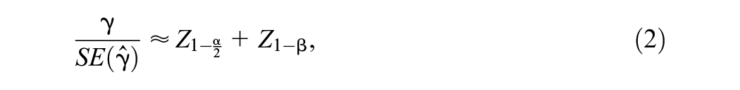
where in our example

which gives a value for the power of
Returning to our simulations, we therefore have two decisions to make: how many simulations do we run, and what do we do with each of the simulated datasets? Here we consider two simulation-based approaches, which we shall refer to as the zero-one and standard error methods. Unlike theory-based methods, which give an exact power estimate, simulation-based approaches are subject to Monte Carlo errors so a slightly different answer will be obtained for each set of simulations. The larger the number of simulations used the smaller will be the Monte Carlo variation. We describe each approach below before comparing their performance for the above illustrative paired
2.1 Zero/One Method
The most used approach in many simulation-based sample packages is what Browne et al. (2009) call the “zero/one method.” Here, for each simulation, we construct a 95% confidence interval for the parameter of interest, the mean improvement in scores in the above example, and determine whether it contains 0. The proportion of simulations for which the interval does not contain 0 is an estimate of the power of the test, denoted by
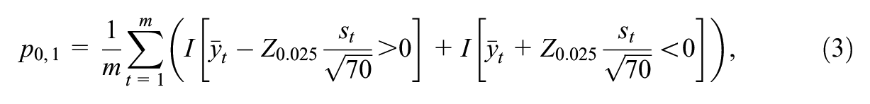
where
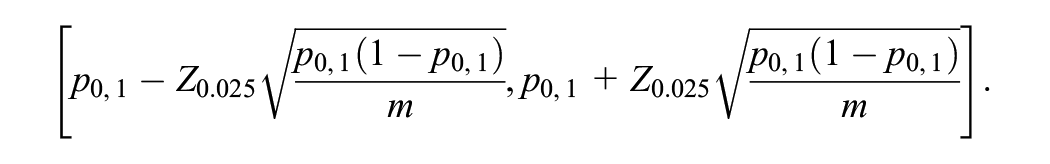
The advantages of this approach are that it is simple to understand and corresponds to what we will do with the real data we collect. Its disadvantage, however, is that it uses the minimum possible information per simulation: if a simulation results in a confidence interval that nearly covers 0 this is treated identically to a confidence interval that is far below or above 0, that is, the proximity to 0 is ignored.
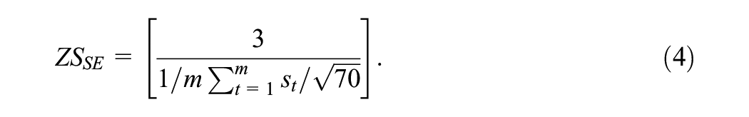
2.2 Standard Error Method
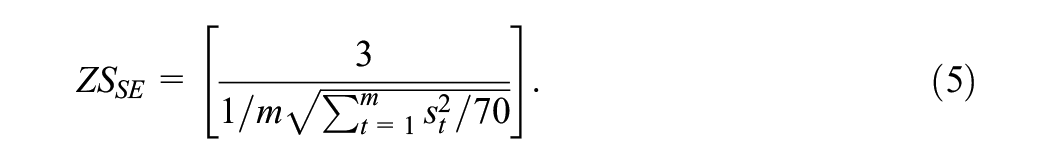
When performing a power calculation, the value assumed for the parameter of interest is known and used in the simulation procedure. Here, we know the underlying mean difference, μ (assumed to be 3 in the example above), and the challenge in power calculations is to evaluate the standard error associated with estimation of μ. The software package PINT simply gives standard errors for the parameter estimates, allowing users to convert them to power estimates should they require. A second approach one might therefore consider, which was first suggested to us by Hox (personal communication 16th April 2007), is the “standard error” or “SE” method where for each simulation we simply record the standard error of the parameter. We can then calculate the average of these standard errors and use this along with the known parameter value to form the z-score and hence the power estimate. For example, with a known mean difference of μ = 3 and sample size n = 70 we would have
In fact, using the mean of the standard errors is not such a sensible idea as for small sample sizes the sample mean is biased (downwards). This is because although the sample variance estimator,
Under the alternative hypothesis then
2.3 Simulation Method Comparison
Both the “zero/one” and standard error approaches take equivalent times to run per simulation so any benefit of one approach over another will be in being able to run it for less simulations. To illustrate this, we vary the number of simulations used from 50 to 5,000 (in steps of 50 to 500 and then steps of 500 to 5,000) and plot Monte Carlo intervals around our estimates to reflect the uncertainty of our power estimate that is caused by the Monte Carlo nature of our procedure. Here, we use a resampling approach by repeating our simulations 1,001 times and from these 1,001 estimates (per simulation size) picking the 2.5% and 97.5% quantiles. Figure 1 plots the resulting Monte Carlo intervals for each number of simulations. We can see that the SE method compared to the 0/1 method reduces the uncertainty to a large degree. The Monte Carlo uncertainty intervals for the 0/1 method require thousands of simulations to be as small as those for the SE method with just 50 simulations.
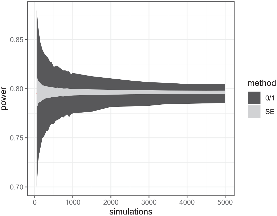
95% Monte Carlo bands for the two approaches to simulated power calculations for different numbers of simulations in a simple single-level model (1).
We could clearly repeat this comparison for more complex multilevel models. The one possible disadvantage of the SE method, over the 0/1 method, arises when we use a procedure that gives biased parameter estimates, which can occur for certain quasi-likelihood estimation procedures that were historically used for discrete responses (Browne & Draper, 2006; Rodriguez & Goldman, 2001). As the variance and hence the standard error of parameter estimates in models for discrete responses is often related to the mean then the SE method involves mixing an unbiased true parameter value with a biased standard error, and this may result in a biased and over-optimistic power curve. We will revisit this in Section 5.3 when we consider a multilevel logistic regression example.
The other consideration is bias in the variance estimator itself as it is well known (Goldstein, 1989) that maximum-likelihood estimation gives biased estimates for variances (particularly for small samples) which in turn results in bias in the estimation of standard errors of fixed effects, and so it will be preferable to use Restricted Maximum Likelihood (REML) estimation to remove this bias, and we will use this in later examples for the SE method (but not for the 0/1 method).
It is clear from this simple single-level example that we can reduce the computational burden of simulation-based power calculations for one particular scenario by switching to the SE method but can we do even better when considering a series of scenarios? We look at this next.
3. Using Simulation Approaches for a Series of Scenarios in a Single-Level Modeling Setting
In Section 2, the SE method was found to reduce the Monte Carlo standard errors of the simulation-based approach to sample size calculations in a single scenario. Typically, however, the motivation for power calculations is to choose between different data collection scenarios, for example, different sample sizes, and to find the sample size at which power first exceeds a threshold (often 0.8). Here simulations for a sequence of scenarios of increasing sample size can be performed and by interpolation the point where the resulting curve crosses the threshold is found.
There are methods to speed up the selection from this sequence, and Price (2017) considered various approaches commonly used in optimization problems to reduce the number of different sample sizes to be evaluated. For example, one can use bracketing intervals, that is, two sample sizes with respectively lower and higher power than desired, followed by bisection or secant methods. Bisection involves repeatedly dividing the set of possible sample sizes in two while keeping the half that contains the optimal sample size. Secant methods similarly reduce the set of possible sample sizes via linear interpolation to home in on the desired sample size (see Price, 2017 for more details). Although these methods will reduce the number of scenarios required to be investigated by homing in on the correct sample size, they still treat each scenario in isolation or in pairs.
Ideally, it would be better to share information across scenarios more generally. One method to do this is to use the power estimates from each scenario and the respective sample size as inputs into a (parametric) modeling approach to fit the power curve. Price (2017) investigated this with the “0/1 method” where a dataset consisting of the 0s and 1s for each simulation and the respective sample sizes considered were used to fit a logistic regression:
where
3.1 Example 1: Single-Level Intervention Example
Here, we take a slightly different approach to Price (2017) as we wish to build on the outputs of the more efficient SE method (rather than the 0/1 method) considered earlier. If we repeat the SE approach for several different sample sizes, this will result in a series of corresponding power estimates that form a power curve. We will illustrate this for our previous intervention example from Section 2, but this time with the number of simulations per scenario fixed at 1,000. The number of students in the sample changes for each scenario from 10 to 100 in steps of five as our aim is to find the minimum sample size that gives a power of 0.8.
The power curve resulting from the simulations can be seen in Figure 2 below.
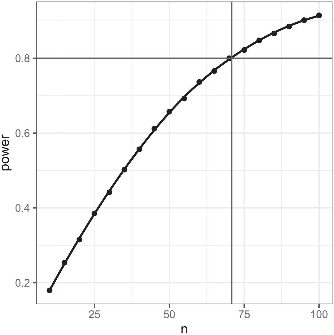
Power curve for the mean difference in scores in the single-level intervention example showing power increasing as sample size (n) increases with sample size for a power of 0.8 identified.
Figure 2 shows a loess (locally estimated scatterplot smoothing) curve formed from the points for each scenario, and we can read off where the curve crosses 0.8 to get the desired sample size. Modeling this curve parametrically is perhaps harder but we can use transformations and the form of the power calculations formula to find an easier relationship to model.
The standard formula for a power calculation is given by (2). For our specific case where the standard error is
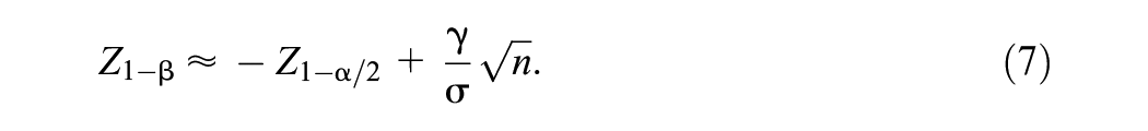
In terms of relating power to sample size, we can see that fitting a linear regression to the z-scores of the power against the square root of sample size should give a straight line fit with the intercept equal to
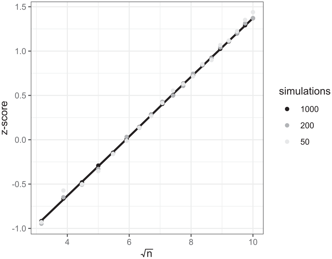
Plots of z-scores against square root of sample size for the intercept parameter representing the mean difference in scores in the intervention example with 50 (in light gray), 200 (in dark gray), and 1,000 (in black), simulations per sample size.
Figure 3 shows a clear linear relationship with the black points from 1,000 simulations per setting lying largely on the line and with increasing Monte Carlo errors as we reduce the number of simulations to 200 and then to 50. This implies that, due to the linear relationship, we could get the same straight line from a smaller number of different sample size scenarios, and as few as only two. This would reduce the simulation time dramatically: Here we have considered 19 different sample sizes so only running two would reduce computation time to about 10% of the full running time. We could also reduce the number of simulations per sample size as an alternative way of speeding up the simulation, but there is a trade-off. For example, if we were to take just the first two sample size scenarios and z-scores for 50 simulations (in light gray) then a straight line joining these two points would be much steeper and diverge dramatically from the black line plotted here. In 7fact, as is well known in the OD literature (Berger & Wong, 2009), if we were to select only two sample sizes, then choosing sample sizes that are further apart will typically result in less error. We will consider these observations in the examples that follow.
4. Multilevel Modeling
4.1 A First Balanced Multilevel Model
We next consider how our first example, model (1) extends to a multilevel setting (example 2). We will generalize the example of a student-level intervention in a single elementary school to multiple schools. Suppose that it is believed that there will be variability across schools in the impact of the intervention and the aim is to detect a smaller effect (2.5 marks) than in example 1 to reflect the likelihood that the school in that example might be more engaged in the process than a school in general. We will again assume a within-school variance of
Here the model for example 2 is

where i indexes students and j indexes schools and we are interested in the power to detect

as a multiplier to scale up overall sample sizes from a single-level model, where
Snijders (2005) gives further design effect formulae for all types of fixed effect parameters in two-level models. These design effect formulae have implications for the speed-ups proposed for the simulation-based sample size calculations in the previous section. We can input the parameter values for our model into the PINT software, and it will produce standard error estimates for the parameter of interest,
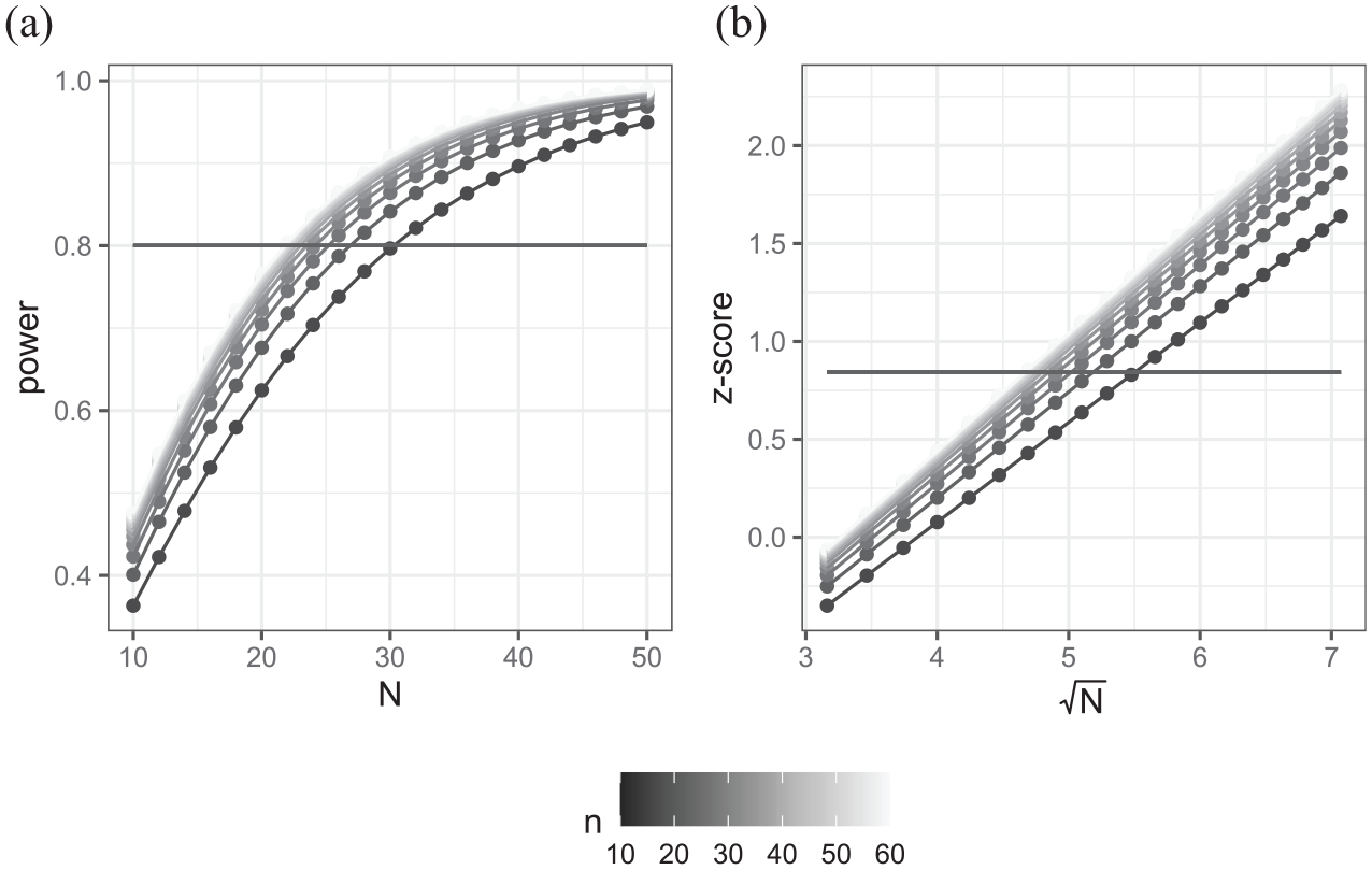
(a) Power curves for example 2 showing power plotted against number of schools with separate curves for different numbers of students per school. (b) Equivalent plot of the z-transformed power against square root of number of schools.
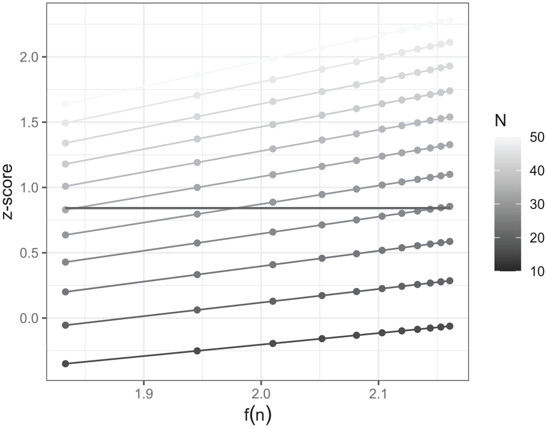
In Figure 4a, we see a series of curves, one for each number of students per school (from 10 to 60 in steps of 5), where we are plotting power against a number of schools. As the number of students per school increases the power curves show higher power. For any given number of students per school, there is a minimum number of schools that will give a power greater than 0.8 (which range from 23 to 31 here). To check whether we can use transformations to get a linear relationship, Figure 4b plots the z-score transformed powers against the square root of the number of schools, and this indeed gives a series of straight lines. For a given number of students per school, we could thus simply choose two different numbers of schools and use them to construct the regression line to give power estimates for any number of schools.
It is worth noting, however, that we might also be faced with the other sample size question of how many students we will need to sample per school for a fixed number of schools. Figure 5 shows the analogous plots for this situation.
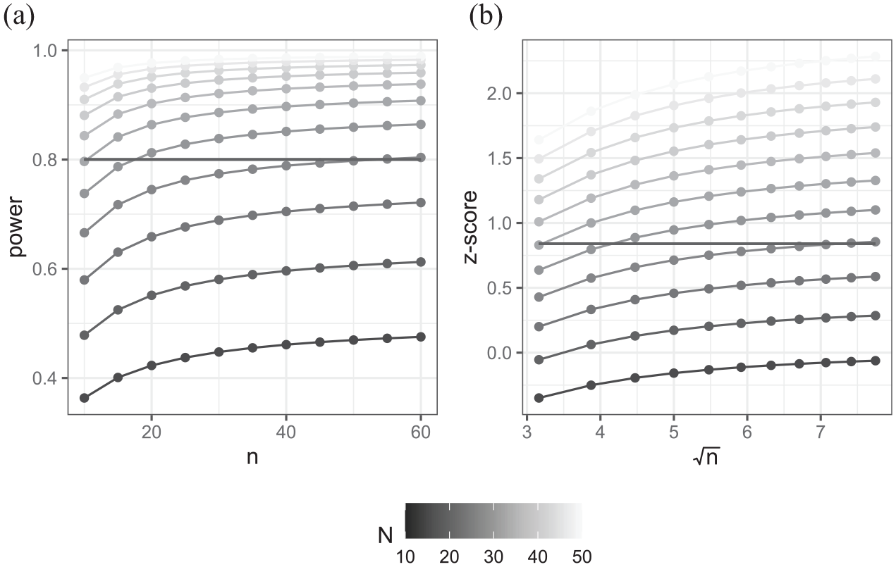
(a) Power curves for example 2 showing power plotted against numbers of students per school with separate curves for different number of schools. (b) Equivalent plot of the z-transformed power against square root of number of students per school.
The power curves in Figure 5a are much flatter than those in Figure 4a. This is in part due to each point on the curve representing an increase of five students (rather than schools) but also the fact that the clustering limits the added value of an additional student but not that of an additional school. In Figure 5b, the intra-class correlation is pulling down the previously straight lines we saw in Figure 4b. In fact, in the extreme case of a purely level 2 response, the lines would become horizontal as there would be no gain in adding students to existing schools (see also Hemmings et al., 2011).
In this simple example, we can in fact calculate a different function of n that will form a linear relationship as we know the standard error of the intercept estimate is
Plot of z-transformed power estimates against
We have shown that, for a variance components model with balanced data, there exist two transformations of the two different sample sizes, the number of clusters N and the number of observations per cluster n, that exhibit linear relationships with the z-score transformation of power. We can therefore use the power estimates from as few as two different sample size scenarios to construct a power curve to find the optimal number of schools for a fixed number of students per school, and for the optimal number of students per school for a fixed number of schools.
We have deliberately considered a simple example here but generally power calculations for the effects of predictor variables are of interest. Snijders and Bosker (1993) generalize standard error estimation for all two-level multilevel models including predictor variables defined at both levels and random slope models. These standard errors can then be used for power calculations for testing the significance of these predictor variables.
In terms of the transformation approach, the linear relationship with the z-score of the power and the square root of the number of level 2 units will hold in each case. For the alternative sample size question regarding the number of level 1 units to choose per level 2 unit, it should also be possible (by rearrangement of the formulae in Snijders, 2005) to construct a function of n that exhibits a linear relationship with the z-scores. Interestingly, for the random intercept model, the relationship will depend on properties of the predictor variable. In two-level random intercept models where the predictor is purely a level 1 predictor, that is, does not vary across level 2 units, then the linear relationship will be with
What is interesting is that even though things can get more complicated we can typically rearrange the formula to be of the form
Although looking at these functional forms is interesting as it gives insight into how the multilevel model inflates standard errors to account for clustering, PINT will instantly give the standard errors required and so there is little need for simulation-based methods here. We will therefore in Section 5 look at examples outside the balanced two-level normal response models that PINT covers. First, however, we will perform a simulation study to compare possible methods for speeding up the simulation-based approach in the context of the current example.
4.2 Simulation Study to Assess Performance of Different Simulation-Based Approaches
In Section 4.1, we illustrated how transformations of power curves can result in linear relationships and hence can be indirectly used via a linear regression fit to obtain parametric estimates of power curves using all the data from a series of scenarios. In this section, we will now look at this in more detail via a small simulation study.
We return to our education example of Section 4.1 but focus on one specific sample size question. Let us assume our educational intervention is to be performed in multiple schools by a single team that will visit each school in the study on a single day per school but only have capacity to perform the intervention on 20 students during that time. The question, therefore, is how many schools they should visit and this amounts to examining the power curve for 20 students in Figure 4a and finding where it crosses 0.8.
In PINT, we can consider a large range of numbers of clusters as it estimates standard errors instantly. In contrast, when using simulation, the computation time will depend on how many scenarios we consider so here we will only estimate power for numbers of clusters from 10 to 50 in steps of five. This will result in nine scenarios. As mentioned in Snijders and Bosker (1993) the standard errors from PINT are large sample approximations; more generally the standard errors will depend on the estimation method that we use for the model fitting. Here we use the lmer function in the lme4 R package and choose the slightly larger REML estimates as the SE method requires unbiased standard error estimates. We now describe three different methods to utilize the results of our simulation.
Method 1: Consider the (perhaps standard) approach of treating the nine scenarios in isolation and recording the power for each. As the power estimates should increase with the number of clusters, find the two scenarios that bracket a power of 0.8 and use linear interpolation to find the smallest number of clusters with power >0.8.
Method 2: Take the z-scores for the two scenarios from the furthest apart sample sizes (10 and 50 schools) and fit the regression line through these two points against the square root of the number of clusters. Use the resulting linear regression line to predict the minimum number of clusters that has a power greater than 0.8.
Method 3: Take the z-scores for the nine scenarios that correspond to the power estimates and fit a linear regression of these z-scores against the square root of the number of clusters. Use the resulting linear regression line to predict the minimum number of clusters that has a power greater than 0.8.
Methods 1 and 3 use the full dataset whilst method 2 will reduce the time of the simulations as it only needs to run simulations for two out of the nine scenarios.
For each of the three methods, we report results using the SE method here noting that similar improvements over the 0/1 method can be observed for this example as earlier. As we are interested in speeding up the simulation procedure, we will also consider three different numbers of simulations (50, 200, and 1,000) per scenario. If we consider 1,000 simulations as a reference, we will be speeding the exercise up by factors of 20 and 5, respectively. This results overall in nine different method combinations in total. The simulation exercise was performed 100 times using different random number seeds to investigate the repeatability of the different methods in terms of which number of clusters they propose. The simulations were performed using R code modified from that created by MLPowSim for similar models but also using the R parallel package to run replications in parallel. Running 8 replications in parallel on a 3.80 GHz 8 core PC with 8 GB of RAM took 1 hour 25 minutes to run the 100 replications. Figure 7 illustrates the results of the simulation experiment:
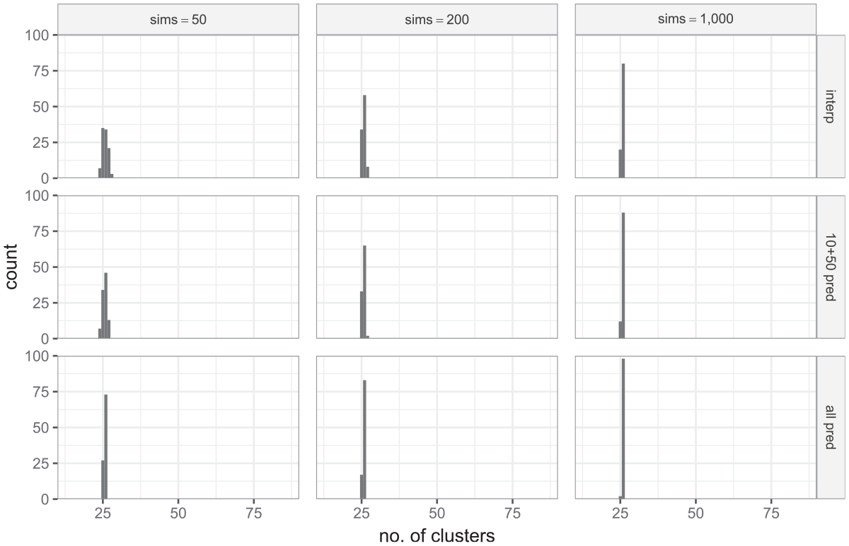
Estimated number of clusters required from simulation study with 20 students per class. The columns of graphs represent three different numbers of simulations per scenario. The rows in the graphs are in the order of methods 1 through 3.
Starting at the bottom right graph of Figure 7, we see that for 1,000 simulations per scenario and the regression method (method 3) we get the anticipated behavior with the same number of suggested clusters (26) for 98 of the 100 replications. The other 2 replications opt for 25 clusters which given from theory the power for 25 clusters is 0.797, is perhaps not unexpected given the Monte Carlo nature of the method. If we reduce to 200 simulations, we get 26 clusters 83% of the time but a decrease to 50 simulations per setting leads to a little more variation in sample sizes with only 73% of replications giving 26 clusters.
In a similar way, a decrease in the number of scenarios leads to a small reduction in performance. Using only the 10 and 50 clusters data (method 2) does well: for 1,000 simulations it also gives 26 clusters 88% of the time but drops off to 65% and 46% when simulations are reduced to 200 and 50 simulations respectively.
The more standard interpolation approach (method 1) does reasonably well with 80% of replications giving 26 clusters for 1,000 simulations with 58% and 34% of replications giving 26 clusters for 200 and 50 simulations respectively; its performance is similar to, but not quite as good as, method 2 but requires all the data. It should be noted that for method 1, we are using linear interpolation between the two bracketing sample sizes, and it is possible, therefore, that applying a smoothing method such as loess on the whole set of points may do slightly better.
We have focused on one example for our simulation study in this paper, though we have observed similar results for other examples. In summary, these simulations have shown the following:
The approach of fitting a regression of the z-scores against the square root of number of clusters appears to improve accuracy over a more standard interpolation of the power estimates. We will look in the next section at which more complex multilevel models this method can be generalized to.
In terms of speeding up the simulations, the two approaches of reducing the number of simulations per scenario and the number of scenarios used in the regression will both reduce, to a degree, the accuracy of power estimates, but will greatly speed up the procedure.
Software implementations of analytical formulae can be used to calculate power estimates for the simple multilevel model considered here to calculate power estimates. In the next section, we consider further, more complex examples to explore whether there are still linear relationships that will reduce the time required.
5. More Complex Multilevel Power Calculations
In this section, we consider three scenarios that are not covered by PINT, but that can be implemented in simulation-based packages like MLPowSim. We show that for certain optimization problems, the regression-based approach can still be used to improve the accuracy of the calculations and reduce computation time.
5.1 Three-Level Modeling Example
A restriction of the theory-based PINT package (although not the OD or SPA-ML software) is that it can handle only one level of clustering, that is, a two-level model. This is not to say that analytical formulae cannot be used for three-level scenarios, indeed Moerbeek et al. (2000), Konstantopoulos (2008), and de Jong et al. (2010) among others discuss such theory and some recent theory-based power calculators include three level designs. As an alternative approach Van Breukelen (2024) looks at equivalences between three-level, two-level, and one-level designs to allow the use of simpler power calculators.
Continuing with our within-school intervention example, suppose that to generalize from the specific teaching conditions experienced within a single classroom it is decided to sample five children from each of four classes rather than 20 students from one class. We now have a three-level structure with children nested within classes nested within schools. For illustration, we have fixed the number of students and classes per school and so our sample size question reduces to how many schools we require. We will assume the same anticipated effect of

where
Figure 8 shows the power curve and the plots for the z-scores of the intercept in this model against the square root of the sample size of highest-level units (schools). We can once again see a linear relationship showing that the transformation idea extends to three-level models, in this case for the intercept. As with the two-level model, this relationship with the square root of sample size at the highest level also holds for the coefficients of predictors because adding units at the highest level is not affected by the clustering that occurs within such units. For changes to the number of units at lower levels, the situation is more complex, as described below.
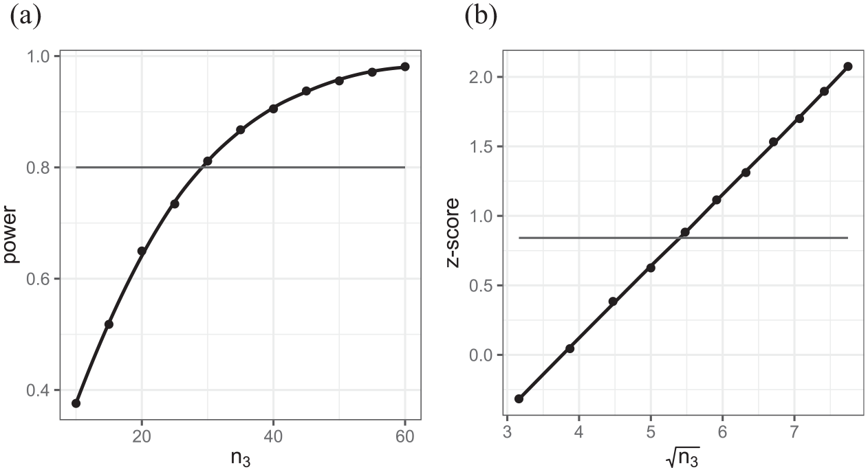
Plots of (a) power versus number of schools and (b) z-scores against square root of the number of schools respectively for three-level example.
We might consider a slight variant of this design where we are constrained to visit 30 schools (n3) and we want to determine how many classes (n2) we should include in each school: choosing between two and eight classes and sampling five children from each or choosing four classes but varying the number of children (n1) from 2 to 10 in each class.
For our simple three-level variance components model, the standard error for the intercept estimate is
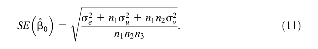
We can see immediately that when varying only the number of schools
In terms of changing the number of level 2 units
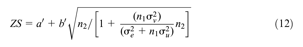
for some values
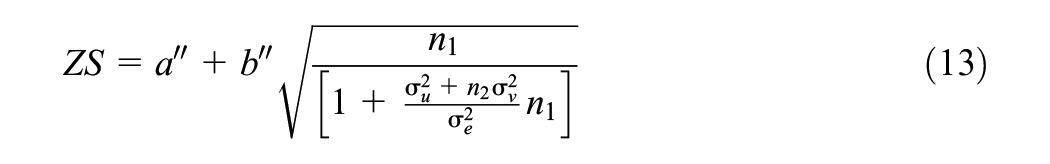
for some values
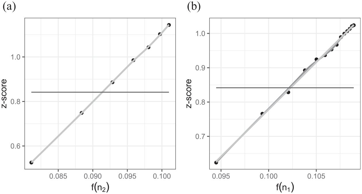
Plots of (a) z-scores versus derived function of number of classes (level 2) and (b) z-scores versus derived function of number of students (level 1) in the three-level example where we allow numbers of classes and numbers of students to vary respectively.
Figure 9 shows the z-scores calculated using Equations 12 and 13, respectively, using 5,000 simulations per combination of sample sizes to smooth the fit. The linear regression fit is shown in light gray and a loess smoother fit in black.
It is worth noting that these variance components models are special cases of more general three-level models. de Jong et al. (2010) give matrix formulae for some specific extensions to the models considered here (including predictors at lower levels and random slopes) that also involve summary statistics for predictor variables in the model. What is clear is sample size optimizations that involve varying the number of highest-level units are the most straightforward in that the simple idea of plotting z-scores against the square root of the number of highest-level units holds. In fact, as with the two-level case, the relationship with the square root of sample sizes will also hold for estimating power to detect purely level 1 predictor variables, that do not have an associated random slope, when varying any one of the three sample sizes but this does not hold for other predictor types. For the optimization problems involving varying the number of units within clusters or the number of lower-level clusters, we have shown that formulae can be used to obtain linear relationships in the variance components case, and it should again be possible to generalize to models with predictor variables and random slopes albeit the formulae will be more complex.
5.2 A Cross-Classified Unbalanced Example With Control of One Classification
A common challenge in designing educational studies is that there are often clustering factors that can be hard to control in sample selection. For example, to extend our current example, let us suppose that the intervention is carried out in the first year of middle school. We might employ our sample design from Section 4 by taking a number of students from a chosen number of (middle) schools. Our sample size questions would be how many schools and how many pupils per school; however, prior educational experience might be equally important but harder to control. In the United Kingdom, for example, students move from primary school to secondary school at age 11 and it is common for secondary schools to take their intake from several primary schools as they tend to be larger. It is also common for children from the same primary school to go to different secondary schools so primary schools are not nested within secondary schools. Whilst it is generally easy to discover which primary school each child attended it is often impractical to build this information into sample selection. Therefore, we could envisage a study design where we choose pupils at random from a number of secondary schools and then simply note their previous primary school so that we control for any primary school clustering in our modeling. In particular, the impact of primary school clustering will often be greater than that for secondary school clustering for data collected at the start of secondary school because those schools will have taught the children for a longer period.
In order to replicate this scenario, we use the structure of a dataset from Fife in Scotland (Paterson, 1991) that is often used as an example for cross-classified models. The full dataset has 148 primary schools that serve 19 secondary schools. We assume that we wish to collect data from all 19 secondary schools but need to decide how many pupils to sample from each school (we will look at possible scenarios with between 4 and 30 pupils in each school).
We will use the real Fife data (see Supplemental Materials 3 in the online version of the journal) to construct probabilities, for each secondary school, of attendance at each of the 148 primary schools and use these probabilities in our simulation to generate the primary schools associated with each pupil. Let us assume the original anticipated intervention effect of
The model (using the notation of Browne et al. (2001) developed for the more general Multiple Membership Multiple Classification family of non-nested model) takes the form


where
If we follow the approach used in the three-level hierarchical example in Section 5.2 then we expect to find a linear relationship between the z score of power and a function of sample size of the form
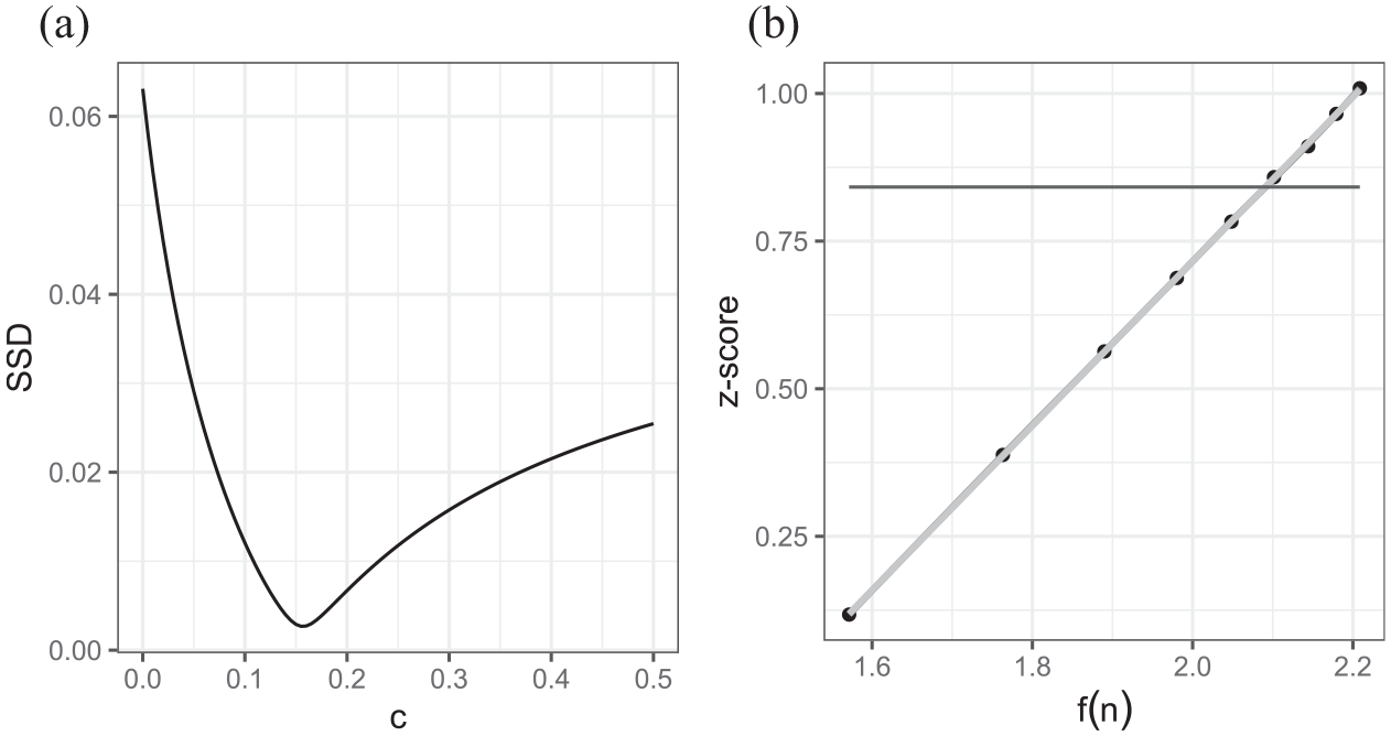
Plots of (a) the sums of square differences for different values of c showing a minimum at around .155 and (b) z-scores versus the resulting derived function (using c = .155) of number of schools in the Fife cross-classified example.
5.3 Multilevel Logistic Regression Analysis Example
For our final example, we look at power calculations for discrete response multilevel models. Such models are covered from an analytical perspective by Moerbeek et al. (2001) using marginal quasi-likelihood (MQL) and are considered in the OD software package. These methods are also specific to MQL (that is less commonly used today due to its known biases) although Moerbeek et al. (2001) derive an adjustment for penalized quasi-likelihood estimation and numerical integration. Power calculations for multilevel logistic regression models can be evaluated by MLPowSim and have also been investigated by Ali et al. (2019) using simulation-based approaches.
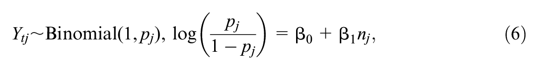
We consider an example with a binary outcome for passing or failing a test. Let us suppose we have a test where historically 50% of students pass, and we wish to see whether a particular teaching intervention can improve the pass rate. We will evaluate this intervention in a number of schools, and we expect the post-intervention pass rate to increase to 60%, that is, an intervention improvement of 10 percentage points from the baseline of 50%. Note that this is not the optimal design for such an intervention as in practice we would likely match the pre and post pass/fail indicators for individual students but it allows us (for simplicity and consistency) to continue with designs that can be analyzed with a model containing only an intercept parameter.
We fit a logistic regression model to the post-intervention scores and compare the estimated mean to 50%, which corresponds to comparing the estimated intercept to 0 (the logit transform for .5). We assume there is between-school variability in the post-intervention probability of a pass that equates to a variance of
Our model is therefore
where
One of the challenges with multilevel logistic models is deciding on which estimation procedure to use. Rodriguez and Goldman (2001) showed that the quasi-likelihood methods that were originally developed for fitting such models give very biased estimates when the outcome is rare, clusters are small, or clustering is severe, with the intercept and between-cluster variance both biased toward zero. Browne and Draper (2006) also confirmed this and showed how MCMC methods performed better. Other more computational methods like adaptive Gaussian quadrature (AGQ) are now commonly implemented in software and here we use adaptive quadrature in R via the glmer function (Bates et al., 2015). In the implementation in glmer, the user can choose the number of quadrature points with the more points chosen the better the approximation. Here we consider values of 0, 1, and 3 for the function. One quadrature point is equivalent to the Laplace approximation and choosing the value 0 gives a fast algorithm that is less accurate but converges more often.
Figure 11 shows the results when a value of 0 is used, while Figures 12 and 13 show the equivalent graphs when the number of quadrature points shifts to 1 and 3, respectively. What is clear when using the value 0 for quadrature points is that the bias in the point estimate for
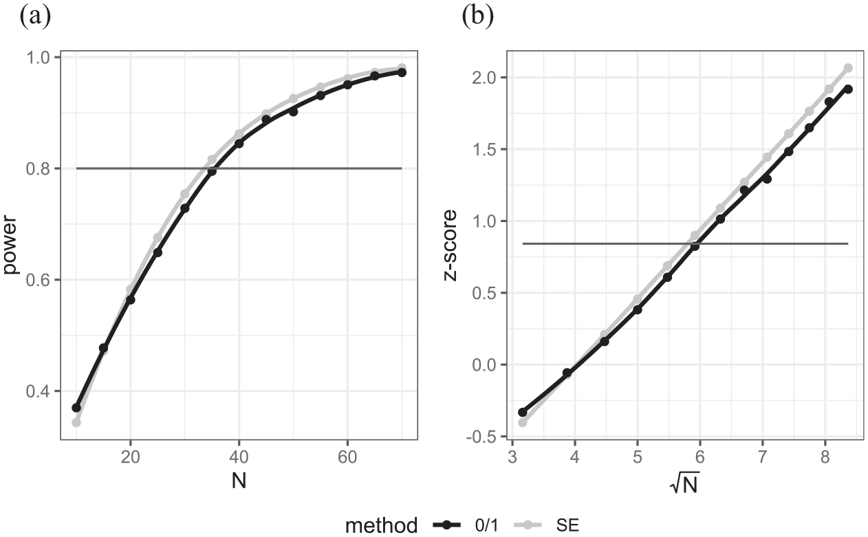
(a) Power curves versus sample size for case where AGQ = 0, (b) z-transform of power vs. square root of sample size.
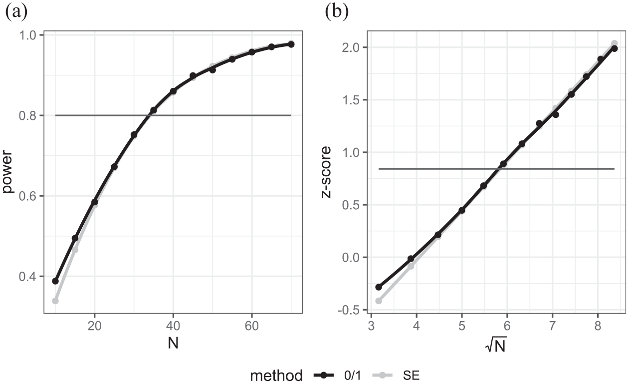
(a) Power curves versus sample size for case where AGQ = 1, (b) z-transform of power vs. square root of sample size.
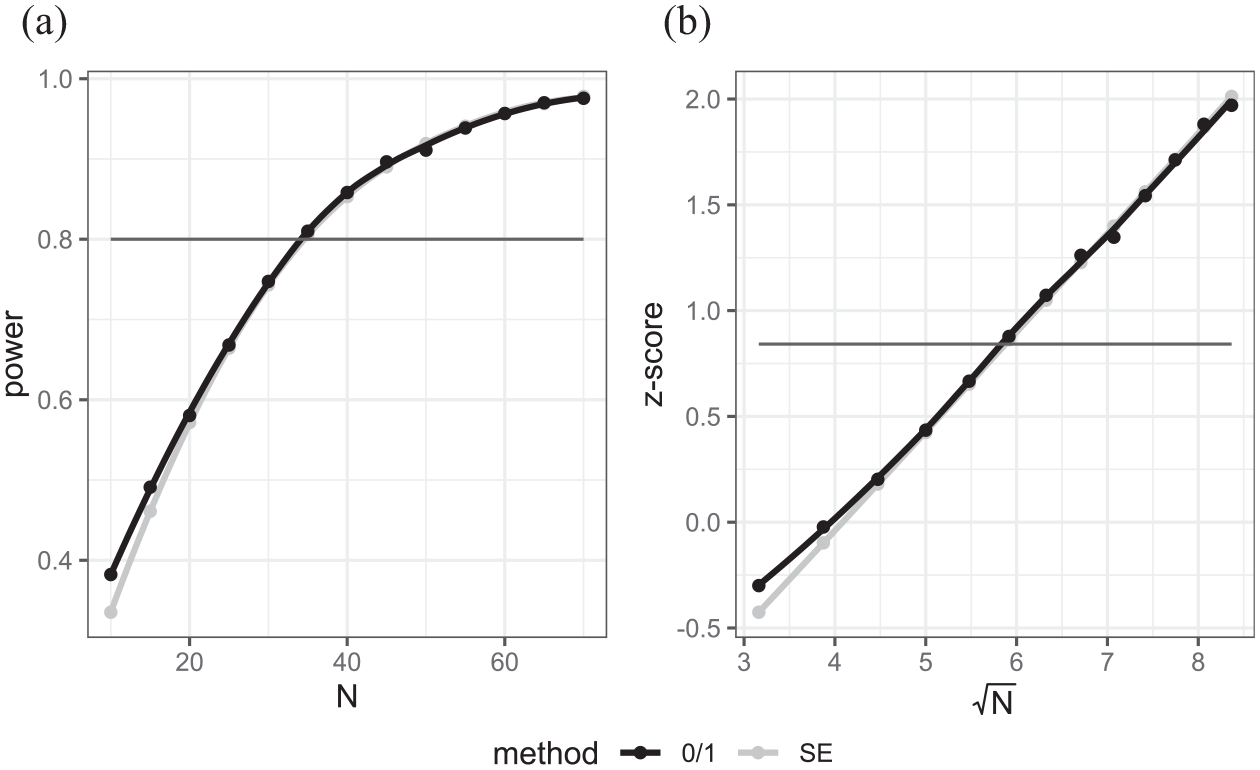
(a) Power curves versus sample size for case where AGQ = 3, (b) z-transform of power vs. square root of sample size.
In terms of the use of the transformation—the estimates from the SE method (in light gray) in Figure 11b look plausibly linear whilst the 0/1 function exhibits some non-linearity.
When the number of quadrature points increases to 1 and 3, we see much closer agreement between the SE and 0/1 methods. Interestingly moving from 1 to 3 quadrature points only makes a small difference here as we are modeling in a situation where the approximation is good (underlying probability close to .5, ICC low and cluster size large). In fact, seven quadrature points (not shown) give a fit very similar to three quadrature points. What is interesting is both the SE and 0/1 methods have broad agreement on power for sample sizes where power ranges from around 0.5 to 0.9 but the 0/1 method transformation still exhibits a slight curvature in the tails (Figures 12b and 13b). Now that the two methods agree, they give a suggested sample size of approximately 34 schools closer to the 33 from the SE method with AGQ = 0 than the 36 of the 0/1 method.
The results for the AGQ = 0 setting are included because it has been reported in several places that for more complex models only the AGQ = 0 setting will converge in the glmer package and so here we show that with this method (and indeed for quasi-likelihood methods in other packages) the SE method may give more optimistic sample size estimates than the 0/1 method.
6. Discussion
In this paper, we have looked in more detail at the choice’s researchers face when using simulation to perform sample size calculations. We have divided these choices into decisions on how to use the results from the simulations of a single scenario and decisions on how to combine simulations across different scenarios to maximize the efficiency of the procedure.
In general, we have shown that compared to the traditional 0/1 method for calculating power for a particular setting, the SE method is more efficient provided an unbiased estimation routine like REML (for normal response models) is used for estimation. The only scenarios where the SE method diverges from the 0/1 method are cases where the estimation procedure is biased, for example, with models for discrete responses using some approximate estimation routine like Quasi-likelihood or AGQ with low numbers of quadrature points. In these situations, we would recommend using a less biased estimation routine, if possible, for example, second-order Penalized Quasi-likelihood or AGQ with more quadrature points.
When we come to consider a set of scenarios, for example, a set of possible sample sizes, we have shown that there is merit in finding functions of the underlying power and the sample sizes that exhibit linear relationships. In fact, in many scenarios, plotting against the square root of the number of clusters at the highest level gives such a relationship. It is then possible to reduce the number of scenarios that need to be simulated to calculate the desired sample size estimate. This will be increasingly important as the underlying models to be fitted become more complex and thus take longer to fit.
In Section 4.2, we performed a simulation study to compare different approaches. The results showed that there is a trade-off between reducing the number of simulations we run and the accuracy of the power calculation. The simulation was designed to confirm that we can get reasonable performance with just two scenarios but that choosing scenarios further apart is better than those close together. An alternative is to increase the number of scenarios while reducing the number of simulations for each. In terms of future work, it would be interesting to consider an optimal simulation design here, perhaps with different numbers of simulations for different scenarios to reflect the differing uncertainty at the different sample sizes. We could also consider how such simulations can combine with or compare to the work in Price (2017) that iteratively chooses better guesses at the optimal sample size.
For the majority of the models considered in this article, it is possible to use theory to perform the power calculations without needing simulations either directly with software implementations or via coding up existing formulae. We have deliberately chosen such models not because we believe it is better to use simulation in these cases but to confirm agreement between the theory-based and simulation-based methods. We would advocate expanding the range of models where theory-based methods are implemented in standard software. It is however useful to confirm that simulation-based approaches agree with the theory when it is available.
In Section 5, we have looked at more complex examples to motivate a general form for our proposed linearization method and then used it when theory-based approaches have not been implemented. We have shown that the approach of using the SE method and looking for linear relationships still holds for improving the speed of the simulation-based approach. We have only scratched the surface here to show that the suggested techniques have wider applicability.
We note that all our examples are random intercept models, and clearly more work is needed to verify that models with random slopes and indeed longitudinal models with more complex dependence structures can benefit from the approaches introduced.
In all our examples, we have cast our sample size calculations as one-dimensional optimization problems, for example by fixing all bar one of the different sample sizes in the three-level model example in Section 5.2. Often in the literature, the sample size optimization is converted to a cost optimization problem (see Cohen, 2005; Shen & Kelcey, 2020; Snijders & Boskers, 1993) by including different costs for collecting data at different levels of the model, for example having a cost for each school included in the data collection and a different cost for each child which again creates a one-dimensional optimization. We have not considered such problems here, but they often break down to two-step procedures where, for example, the first step is to calculate the minimum number of schools required for each specific cluster size to achieve a power of greater than 0.8 and the second step is to choose the optimal cost from this set of optimal numbers of schools. Here our approach could be used straightforwardly in step 1.
To conclude, it is worth remembering that as study designs become more complex, sample size calculations require estimates for many parameters, all of which have some uncertainty. This means that although we are aiming to get an exact and consistent estimate of the required sample size, it relies on the parameter estimates used and so is just a guide. If different methods give slightly different sample size estimates, this should be balanced with the uncertainty in the parameter estimates themselves.
Supplemental Material
sj-docx-1-jeb-10.3102_10769986251344939 – Supplemental material for Optimizing the Use of Simulation Methods in Multilevel Sample Size Calculations
Supplemental material, sj-docx-1-jeb-10.3102_10769986251344939 for Optimizing the Use of Simulation Methods in Multilevel Sample Size Calculations by William John Browne, Christopher Michael John Charlton, Toni Price, George Leckie and Fiona Steele in Journal of Educational and Behavioral Statistics
Footnotes
Declaration of Conflicting Interests
The author(s) declared no potential conflicts of interest with respect to the research, authorship, and/or publication of this article.
Funding
The author(s) disclosed receipt of the following financial support for the research, authorship, and/or publication of this article: The work in this paper builds on earlier work supported by the UK Economic and Social Science Research council grants ES/F031904/1 and RES-00-23-1190-A.
Authors
References
Supplementary Material
Please find the following supplemental material available below.
For Open Access articles published under a Creative Commons License, all supplemental material carries the same license as the article it is associated with.
For non-Open Access articles published, all supplemental material carries a non-exclusive license, and permission requests for re-use of supplemental material or any part of supplemental material shall be sent directly to the copyright owner as specified in the copyright notice associated with the article.