
Abstract
Profile analysis is one of the main tools for studying whether differential item functioning can be related to specific features of test items. While relevant, profile analysis in its current form has two restrictions that limit its usefulness in practice: It assumes that all test items have equal discrimination parameters, and it does not test whether conclusions about the item-feature effects generalize outside of the considered set of items. This article addresses both of these limitations, by generalizing profile analysis to work under the two-parameter logistic model and by proposing a permutation test that allows for generalizable conclusions about item-feature effects. The developed methods are evaluated in a simulation study and illustrated using Programme for International Student Assessment 2015 Science data.
Keywords
1. Introduction
In many applications of cognitive testing, one of the main aims of administering these tests is to obtain comparable results for different groups. A crucial requirement for being able to make meaningful comparisons across groups on scale scores involves measurement equivalence or measurement invariance, meaning that the measured construct ought to be understood and measured equivalently across groups (Meredith, 1993). In practice, researchers generally adopt one of the two approaches when examining score comparability: multiple-group confirmatory factor analysis (MG-CFA; Jöreskog, 1971) or differential item functioning (DIF)-type approaches to testing measurement invariance (for an overview of such methods, see Millsap & Everson, 1993; Penfield & Lam, 2000; Potenza & Dorans, 1995). One area in which measurement invariance is especially important yet challenging to establish is in international large-scale assessments (ILSAs), which are generally low-stakes, comparative, population-level assessments and surveys administered across countries that differ in geography, culture, and economic development. The number of unique populations and the size of these studies make this a rich and important area for studying measurement invariance. Over the course of ILSAs such as the Programme for International Student Assessment (PISA) or the Trends in International Mathematics and Science Study (TIMSS), substantial evidence around the cross-cultural differences in achievement measures such as math, science, and reading exists (Grisay & Monseur, 2007; Kankaraš & Moors, 2014; Kreiner & Christensen, 2014). Detecting DIF across countries is important as not accounting for DIF can distort international comparisons: It has been shown that the country rankings are not necessarily robust against the violations of measurement invariance (Kreiner & Christensen, 2014; Rutkowski et al., 2016).
Specific operational methods for identifying measurement differences in the ILSA context are varied and depend on the study and the responsible contractor. For example, DIF analyses in early cycles of PISA were based on the comparisons of national and international relative item difficulties, where especially deviant items were identified as dodgy and either not used for scoring of individual countries or removed altogether for scoring (Organization for Economic Co-Operation and Development [OECD], 2014a). In contrast, the Teaching and Learning International Survey analyses are based on MG-CFA and emphasize the scale level (OECD, 2014b). In recent PISA cycles, measures that quantify deviations in observed data from estimated item characteristic curves are used (Oliveri & von Davier, 2011; OECD, 2020). Once identified, a natural line of investigation surrounds seeking explanations for measurement differences, which is especially relevant in the ILSA context, where dozens of countries are measured on hundreds of items, creating a substantial challenge for summarizing such multivariate results. This context also offers opportunities for pattern detection and for developing cultural or content-related profiles. Studying DIF patterns in ILSA is important not only for DIF detection and treatment but also for studying substantive differences between educational systems in different countries, which is both practically and theoretically important.
In an effort to understand potential sources of cross-cultural measurement differences, studies posited pedagogical traditions, language, or item type. For example, researchers argued that the conceptual nature of teaching in Russia as compared with procedural teaching methods in English-speaking countries explained item-by-country interactions (i.e., between-country DIF) in PISA (Kjærnsli & Lie, 2004). Similar research showed evidence of cultural item response patterns based on geography or language (Zabulionis, 2001). The previously cited studies rely on correlations of item residuals submitted to cluster analysis, with clusters given cultural or other meanings imbued by the researcher.
One important direction for studying the structure of DIF is to consider item features as a possible explanation. In the current context, we use the term item features to describe the characteristics of the test items, such as cognitive demand (high, medium, or low), item format (multiple-choice or open-ended), content dimension (algebra, numbers, or geometry in mathematics), and so on. For example, in the mathematics education literature, there is evidence that girls do better than boys under certain test conditions or on certain topics and vice versa (Hyde et al., 1990; Leder, 1992; Mendes-Barnett & Ercikan, 2006; Liu & Wilson, 2009). It is also important to note that such differences should be regarded not only as deviations from measurement invariance but also as differences between the groups that can be of substantive interest. Studying item features in the context of large-scale assessment is logical because these item features are typically built into the assessment design of the studies, rather than being ancillary or post hoc features of the test. Interested readers are encouraged to see, for example, PISA framework documents for complete details (OECD, 2017). Similarly, TIMSS or PIRLS frameworks are illuminating in this regard (Mullis & Martin, 2017, 2019). At the national level, the U.S. National Assessment of Educational Progress (NAEP) is similarly designed with item features that are built into the framework (National Assessment Governing Board, 2019).
Descriptive approaches have been used to study the structure of DIF in ILSA in relation to item features. For example, Bundsgaard (2019) analyzed item features in the International Computer and Information Literacy Study by first estimating item-level DIF parameters and then looking at items grouped by content domain to identify the patterns of DIF by country. Similarly, to describe differences in the relative strengths and weaknesses of different groups of countries, Olsen (2005) looked at the relationship between item features in PISA 2003 and deviations of the country-specific to international probabilities of correct responses to the test items. Such studies, however, do not take the uncertainty about the DIF-measures (item-level DIF parameters or deviations of the probabilities of correct responses) into account and therefore do not allow statistical inferences about the effects of item features. Rather, such findings provide a descriptive picture of the structure of country differences.
One method used to investigate how DIF is related to item features that does take uncertainty about DIF into account is profile analysis (Verhelst, 2012). In profile analysis, the aim is to study whether a particular group (e.g., country) performs notably better or worse than can be expected under measurement invariance on a set of items with certain features compared to a complementary set of items without these features (e.g., multiple-choice compared to open-ended items). This method conditions on the total number of correct responses and is developed under the Rasch modeling framework (Rasch, 1960), where it is possible to analytically derive the expected number of correct responses to items in a certain set, given the total number of correct responses. Using this expectation, one can classify each person as either performing above or below expectation on the set of items and aggregate these results on the group level. For each group, one can compute the expected and observed frequencies of persons with above- or below-expected performance on the set of items. A significant difference between observed and expected frequencies in a group suggests that items with a certain feature may exhibit DIF compared to items without the feature. For example, one could find evidence that for one country, the discrepancy between the performance on multiple-choice items and open-ended items is bigger than expected based on the international results, suggesting that this item feature might explain observed DIF for the studied country. In addition to providing a significance test for each considered group, one can compute the so-called excess percentage, which captures the difference between the observed and expected frequency of response patterns with the above-expected performance on the items in the set. This value is expressed as a percentage of the total sample size in the group. If the excess percentage is positive (negative) then it means that items with a particular feature are less (more) difficult in the group than expected based on the overall (e.g., international) model estimates. This excess percentage can be seen as providing a meaningful effect size measure to gauge the extent to which the item feature can explain observed DIF.
We note that a number of methods, used to describe the multivariate patterns of observations—focused on both continuous (e.g., Ding, 2001) and categorical data (e.g., Culpepper, 2009)—use the term profile analysis. To extract and describe profiles, established methods include multidimensional scaling (Davison, 1994; Ding, 2001), latent profile analysis (Gibson, 1959), latent class analysis (Lazarsfeld, 1950), and cluster analysis (Moses & Pritchard, 1996), among others. Verhelst (2012) distinguishes his approach to profile analysis by noting that profiles are defined at the individual, rather than the group, level; emphasis is on tests that measure a unidimensional trait; profiles describe relative weaknesses and strengths on predefined categories of items; and profiles are highly discrete. In this article, we will use the term “profile analysis” to refer to the method developed by Verhelst (2012) as has been done in multiple studies focused on explaining the structure of DIF in national and international assessments (Saatçioğlu Hamide, 2017; Vaheoja et al., 2019; Verhelst et al., 2016; Yıldırım, 2022).
Notable alternatives to profile analysis are differential bundle functioning (Douglas et al., 1996) and differential facet functioning (Engelhard, 1992). The first approach is aimed at studying whether, conditional on measured ability, the expected number of correct responses on items with a certain feature is the same in the reference and focal groups. This approach is based on the multidimensional DIF paradigm developed by Shealy and Stout (1993), which underlies the SIBTEST procedure (Bolt & Stout, 1996) that is the primary differential bundle functioning detection tool. The second approach is an extension of the linear logistic test model (Fischer, 1973) to DIF. Under this approach, instead of having an item-specific item difficulty in the reference group and item DIF parameters in each of the focal groups (i.e., difference between item difficulty in the focal and the reference group), the differences in item functioning are modeled by parameters that are specific to sets of items sharing a specific feature.
Profile analysis has important advantages over these alternatives. Compared to differential bundle functioning, profile analysis does not require a set of DIF-free items (i.e., items that are assumed to only measure the primary dimension). Moreover, profile analysis can be used for an arbitrary number of groups and does not require the specification of a reference and a focal group. Both are important advantages in a multiple-group setting, where no obvious reference group presents itself, as in the ILSA context. Compared to differential facet functioning methods, profile analysis does not require separate model parameter estimates for each country. This is a clear advantage in the ILSA context, where complex sampling schemes can render per-country sample sizes too small for precise estimates. Finally, profile analysis provides an easily interpretable measure of effect size (i.e., excess percentage), which can be used to summarize and communicate results to stakeholders. All this makes profile analysis a valuable tool for studying the relative strengths and weaknesses of different groups that have taken a test, for example, studying how countries differ in their performance on specific item types in ILSAs.
Despite several advantanges, profile analysis has an important restriction limiting its applicability in large-scale assessments: reliance on the Rasch model or its variants, which assume equal relationship between items and the underlying factor. Given that large-scale assessments such as TIMSS, PIRLS, PISA, and NAEP operationally use a more flexible measurement model (see, e.g., OECD, 2020), extending profile analysis to these contexts is valuable. Our work focuses on this extension, described in detail subsequently, along with an additional development, the context of which we describe next.
Investigating the relationship between item features and DIF allows us to determine whether observed differences between two sets of items on a given test can be attributed to a particular item feature or whether these differences are caused by random sampling variability. 1 In other words, we can investigate whether observed differences are generalizable beyond the immediate test setting—from those items observed on a particular test—to the population of items that share a particular feature. For example: Is one country structurally better in answering multiple-choice items, or is the observed pattern on a particular test administration limited to that setting? In the latter (nongeneralizable) case, differences are only due to idiosyncratic properties of the items in the two sets (e.g., with specific multiple choice items on this test being easier for one country due to reasons unrelated to the item feature).
It is important to distinguish between the results of a specific set of items on a test and the results of those items when applied to the population of items. DIF results, from profile analysis, differential facet functioning, or differential bundle functioning, can reveal if there is a systematic difference between two groups of items on the specific test, but these methods do not necessarily produce results that are generalizable the population level of items that carry a given feature. Importantly, developing generalizable methods can help to develop better measures that are less affected by culture, language, geography, or other demographics. On the other hand, if findings are unique to a test setting, making systematic adjustments to cross-cultural measures becomes an intractable challenge, as adjustments to future test cycles can create a “whack-a-mole” effect, where new measurement differences surface consequently and observed item feature effects do not reoccur in similar ways in other tests. As such, methods that can reveal whether feature-related DIF results can be expected to generalize outside of the test setting are needed. The importance of distinguishing the test-level and population-level results was earlier discussed by Ong et al. (2013).
Hierarchical logistic regression (Swanson et al., 2002), logistic mixed models (Van den Noortgate & De Boeck, 2005; Van den Noortgate et al., 2003) and Bayesian models for DIF (Gonçalves et al., 2013; Soares et al., 2009) can be used to address the issue of generalizability. In these methods, the group-specific deviations of the item parameters from their overall value (e.g., deviation of the country-specific difficulty of the item from its international value) are modeled as random across items and the variability across items is explained by item features included in the analysis as covariates. However, these methods cannot be directly applied in large-scale applications like PISA that include dozens of countries and a complex booklet design. The incomplete design poses challenges to the use of hierarchical logistic regression, where the test sumscore is used as a proxy for the latent variable: Since the sets of items that students respond to are different, their sumscores are not comparable. Furthermore, hierarchical logistic regression and logistic mixed models in their standard implementation are primarily used for application under a Rasch model, whereas many large-scale international assessments use more complex models. Finally, although there is no theoretical challenge in applying these methods when there are more than 50 groups between which DIF can occur, this has not been done to our knowledge and potentially would need some adjustments to the existing software to make it computationally feasible. Bayesian approaches to DIF have also only been applied in the context of comparing two groups, and there is no readily available software for this method for applied researchers to use in large-scale applications like PISA.
Since existing methods that address the issue of generalizability of item-feature-related DIF are not directly applicable in the context of large-scale assessment, it is of interest to develop methods that are easy to use and interpret for researchers in the field. Extending profile analysis to provide generalizable conclusions would fill the current knowledge gap, as it is computationally less intensive (i.e., it does not require estimating country-specific item parameters) and provides an easily interpretable outcome measure (i.e., excess percentage) expressed in terms of the actual performance of students from different groups rather than the estimates of model parameters. In the current article, we develop a straightforward permutation test for profile analysis to detect item-feature DIF that can be generalized outside of the immediate testing situation. Although in this article our application focuses on an ILSA context, our method can be applied readily in many large-scale assessments and other settings, where one wants to study the impact of item features on the performance of different groups of respondents (e.g., gender, ethnicity, or other policy-relevant groups).
The rest of this article is organized as follows. In Section 2, we describe the details of profile analysis in its current form (i.e., based on the Rasch model and with conclusions on the test level). In Section 3, we first generalize the method to the two-parameter logistic (2PL) model (Birnbaum, 1968), which is operationally common in many large-scale assessments, and then propose a permutation test that would allow for generalizable conclusions. In Section 4, we present an illustrative example examining different item features as potential sources of DIF in PISA 2015 Science assessment. In Section 5, we present a simulation study in which we evaluate Type I error and power of the permutation-based profile analysis. This article is concluded with a discussion.
2. Profile Analysis
Profile analysis is based on considering profiles: sets of subscores on test items of different types. Suppose some items in the test have a specific item feature (e.g., high depth of knowledge). We denote this set of items by

The model can alternatively be parameterized with transformed difficulties
An important property of the Rasch model is that the total sumscore, denoted by S, is the sufficient statistic for ability, from which follows that conditional on this statistic, the distribution of the item scores is independent of ability (Fischer, 1995):
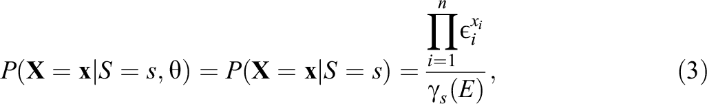
where n is the number of items, E is a set of transformed item difficulties (

For example,
Profile analysis uses a related property of the Rasch model, which has to do with the distribution of the sumscore for a subset of items conditional on the total sumscore. The probability that the sumscore for set

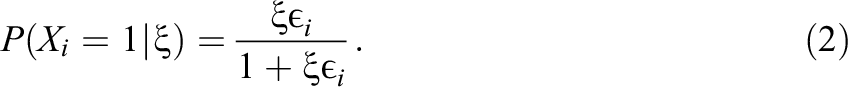
where
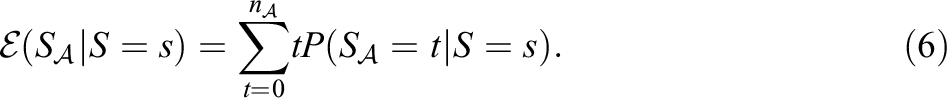
For a single respondent, one can determine whether their observed sumscore for set
In the profile analysis, the observed frequencies of
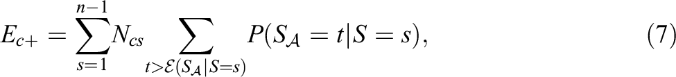
where
Since in the context of many large-scale assessments such as TIMSS and PISA, it is usually impossible to administer all items to all students, and multiple test forms are typically used. In this case, the observed and expected frequencies of
Some deviations of the observed frequencies from the expected frequencies are expected due to sampling variability even when measurement invariance holds. To test whether the observed frequencies are significantly different from the expected frequencies, the

This statistic has a
To compare the deviations between the observed and expected frequencies, Verhelst (2012) suggests to compute the so-called excess percentage:

which is the difference between the observed and expected frequencies as the percentage of sample size (disregarding the trivial profiles).
3. Extending Profile Analysis
3.1. Extension to the 2PL Model
Due to having only one item parameter and assuming that the items have equal discriminatory power, the Rasch model is usually too restrictive to fit real data. Many operational assessments have moved from using the Rasch modeling framework to using more flexible models, like the 2PL model used by PISA since 2015. This model adds a discrimination parameter (

While the total sumscore is not a sufficient statistic for ability in this model, it is still a very important summary of the data that is easy to interpret and easy to communicate to stakeholders, as it still successfully captures overall ability and provides a stochastic ordering of persons. Therefore, a method for detecting item-feature-related DIF that is based on the distribution of the sumscore of items with a certain feature, conditional on the total sumscore is valuable within the context of the 2PL model.
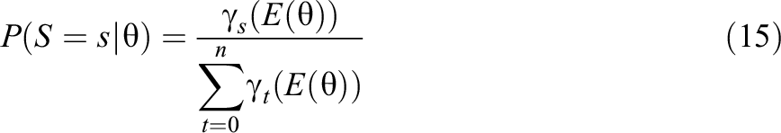
In the 2PL model, the probability of observing a particular value for the sumscore for set

where

The distribution
The integral in Equation 12 can be approximated using numerical integration and considering K quadrature points

The discrete distribution of ability conditional on the total sumscore can be easily computed using Bayes’s theorem:
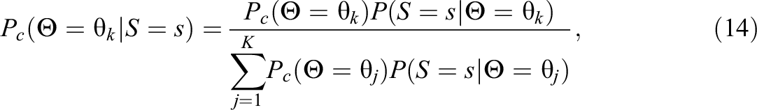
where the distribution of the number of correct responses conditional on ability is
and the probability
The distribution of the sumscore for set
3.2. Generalizability of the Results
In standard profile analysis, statistical inference about the presence of item-feature-related violations of measurement invariance is done by comparing the test statistic from Equation 11 with its distribution under measurement invariance (i.e., a
However, finding such evidence does not necessarily mean that the item features themselves have explanatory power for the violations of measurement invariance. It could also be that violations of measurement invariance on the level of individual items are simply aggregated to the level of sets of items with and without the item feature, and if the test would have included a different set of items with the same features (e.g., in the next cycle of the large-scale assessment study), then there would be no such violation. Thus, the significance test only allows us to draw conclusions about the actual sets of items delivered during a particular test administration (i.e., inference at the test level) and not necessarily about the population of items that have that feature versus the population of items that do not (i.e., inference at the population level). As such, standard profile analysis leaves the question of generalizability unanswered.
To answer the question of generalizability, we propose to add a simple permutation test to profile analysis. Permutation tests are a highly flexible, nonparametric alternative to classical hypothesis tests that operate under a population model. Like classical, parametric null hypothesis tests, permutation tests allow for calculating the probability of getting a value as or more extreme under a null hypothesis. An advantage of permutation tests is that they do not rely on a specific probability distribution. Despite this advantage, they are not, formally, distribution free (LaFleur & Greevy, 2009), since samples are assumed to be exchangeable. The general process of conducting a permutation test involves a random rearrangement of the data followed by recalculating the test statistic of interest. This procedure is repeated either for all possible permutations of the data, referred to as systematic permutation tests, or for a random number of permutations (random or Monte Carlo permutation tests; Huo et al., 2014). The distribution of the resultant statistics is used to derive a p-value, from which inferences are drawn. In the subsequent sections, we provide further details about these procedures. Situations where using permutation tests can offer notable benefits are when sample sizes are small (see, e.g., Camilli & Smith, 1990), when the usual distributional assumptions are not met, or when an exact test is desirable. These methods are also useful when the hypothesis test in question is not about means or medians.
The logic of the proposed permutation test is as follows: If it is likely to obtain the same (or more extreme) value of the test statistic from a random grouping of the test items into sets mimicking the sets “with the feature” and “without the feature,” then there is insufficient evidence to conclude that the actual item feature explains the violations of measurement invariance. Only when the observed test statistic is extreme compared to what is obtained from random permutations of the items into subsets, can we conclude that the observed differences in the behavior of the items from different features are likely to not just be an aggregation of the idiosyncratic characteristics of individual items in the concrete test, but that they have to do with the characteristics of the item features themselves. In this case, we would expect to see the same pattern of violations of measurement invariance if different items with these item features would be included in the test.
More formally, the null hypothesis of the permutation-based profile analysis is that DIF (if present) is not related to the studied item feature (i.e., the null hypothesis is different from that of standard profile analysis). Random permutations of the items into sets produce the null distribution, since DIF is not related to any of these artificial item features created by randomly permuting the items. While in standard profile analysis, the test statistic in Equation 8 is compared to its distribution under measurement invariance, in our permutation-based profile analysis, it is compared it to this new null-distribution, that is the distribution of this statistic across different permutations of the items into random sets (of sizes matching the actual set of items with and without the feature). If the probability of obtaining a value at least as extreme as the observed value is below the specified
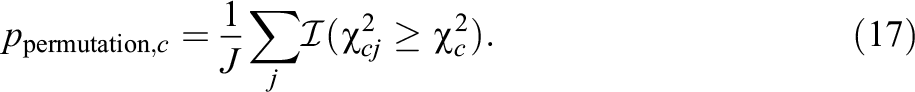
In each permutation

where
When the test consists of multiple test forms, then the permutation of the items is done for all test items. It is first determined which items belong to
In addition to considering the distribution of the
4. Illustrative Example
4.1. Data
Publicly available data from 2015 PISA study were used for analysis. Seventy two countries participated in the 2015 cycle of PISA. To remove any potential mode differences, we only used data from the computer-based assessment, in which 55 countries participated. Because science was the major domain of emphasis, we limit our focus there. From the total of 184 items administered in the computer-based science assessment, there were nine items that did not have any valid responses in at least one of the countries. These items were removed to make country comparisons more straightforward. Furthermore, items with partial credit were recoded to binary items (correct = 1; incorrect or partially correct = 0) to simplify the analysis. Omitted responses were coded as incorrect responses. 2 Only those students who reached all items in their test form were included in the analysis. Further, we omitted responses from students that were administered the Une Heure or UH booklet, which is designed for students with special educational needs (OECD, 2017). Our analysis included 36 different test forms with a minimum of 24 and a maximum of 36 items in them (after the exclusion of the items that did not have any valid responses in one of the countries). The total sample size was 299,240 (with the largest and the smallest sample sizes per country of 17,141 and 1,975, respectively).
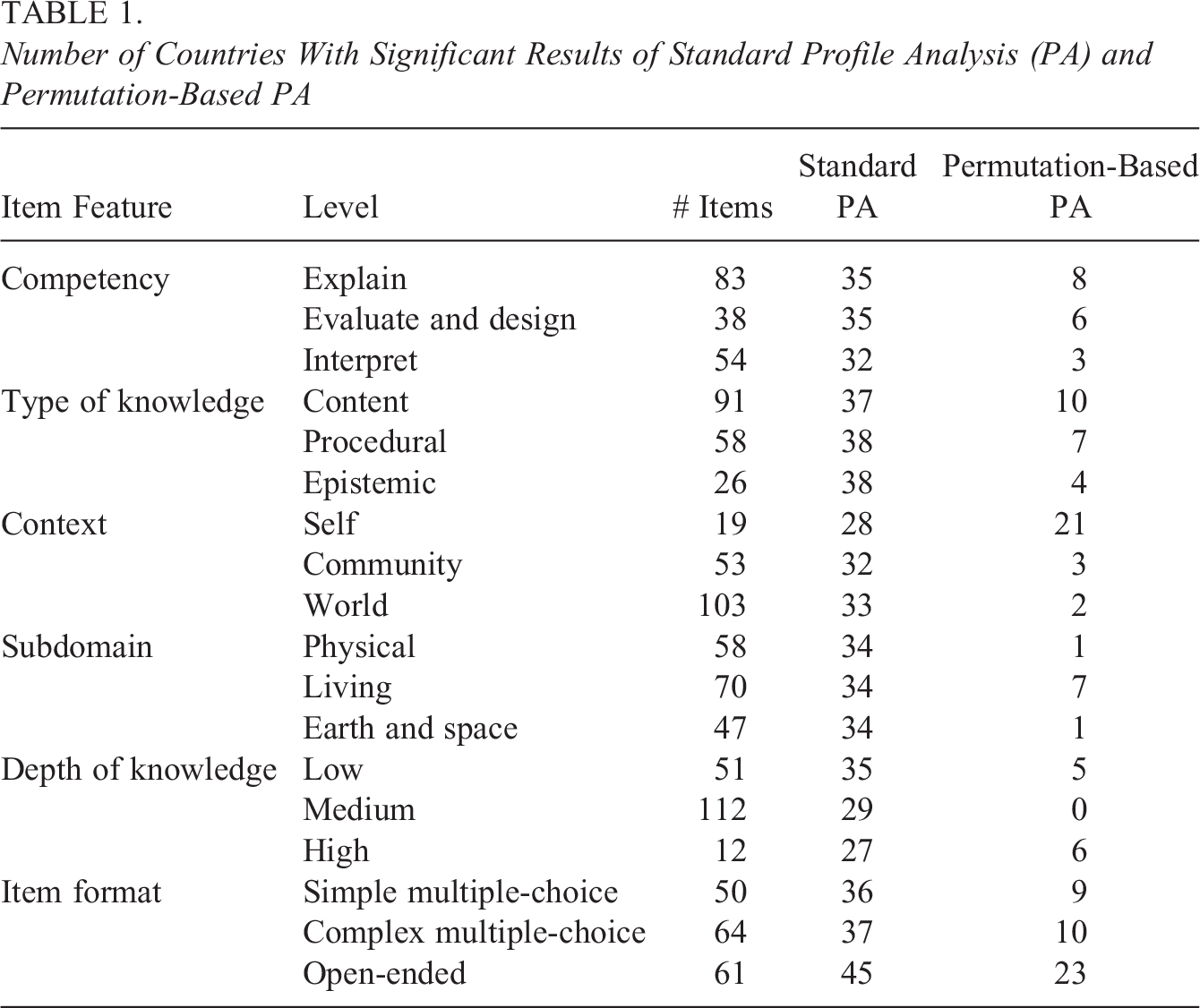
The PISA definition of science literacy is “the ability to engage with science-related issues, and with the ideas of science, as a reflective citizen” (OECD, 2017, p. 20). Based on detailed theories of science learning (see the framework for a full list of references), the science domain and associated items are organized according to several elements. Science competencies is the first element: to explain phenomena scientifically; to evaluate and design scientific enquiry; and to interpret data and evidence scientifically (p. 20). The second element is type of knowledge, which includes content, procedural, and epistemic ways of knowing (p. 19). The science domain further deals with different contexts, that is, situations relating to the self, to the community, or to the world (p. 23). Item content is divided across subdomains, including physical, living, and earth and space systems. Finally, items are characterized by their cognitive demands or depth of knowledge, including low, medium, and high (p. 2). Besides the theoretical science framework used to guide the development of PISA items, items can be further categorized by their item format, with options that include simple or complex multiple-choice items, or open-ended items. See the PISA Technical Report, Annex A for a complete categorization of science items (OECD, 2017). The number of items with each item feature is given in Table 1. For each of these item features, we want to determine whether items having this feature are more or less difficult in each of the 55 countries than expected under measurement invariance.
Number of Countries With Significant Results of Standard Profile Analysis (PA) and Permutation-Based PA
4.2. Method
The multigroup 2PL model with item parameters equal across countries was fitted to the full data set using marginal maximum likelihood implemented in the R package TAM (Robitzsch et al., 2020). The estimates of the item parameters and the means and variances of the distribution of ability in each country were used to perform the 2PL-extension of standard profile analysis and permutation-based profile analysis as described in the previous section. Numerical integration was done using 101 equally spaced nodes between −5 and 5. The analyses were performed for every item feature (each of the three levels of the six item classifications). Permutation tests were performed for each item feature with 1,000 replications. For each item feature and country, we also computed the excess percentage in the observed and permuted data.
4.3. Results
Table 1 shows the results of studying DIF related to item features. For each item feature, one can see in how many countries a significant result was detected (at 5%
Using the results of one country (Australia) on one item feature (type of knowledge: content), Figure 1 presents a graphical illustration of the differences between the test-level inferences done in standard profile analysis and the population-level inferences done in permutation-based profile analysis. The values are presented on the log-scale to improve readability of the plot. The same observed
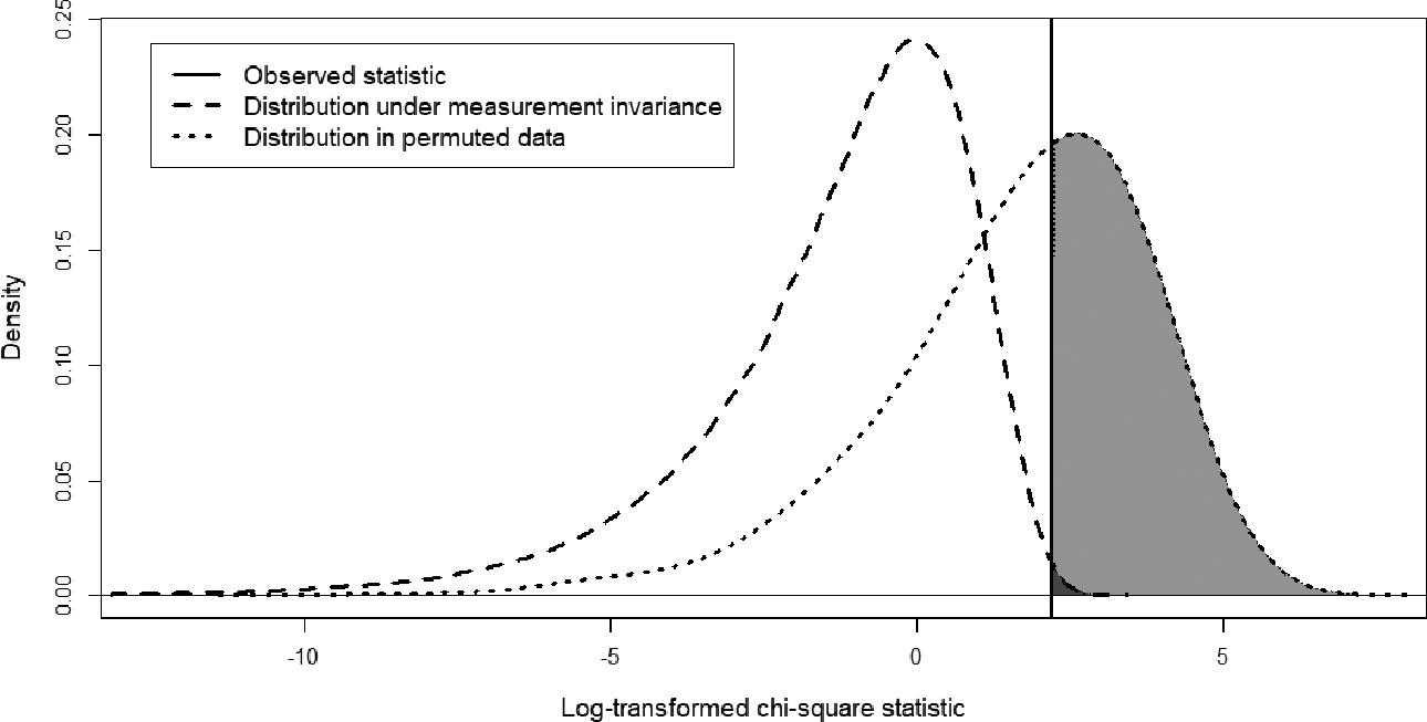
Graphical representation of the differences between test-level and population-level inferences: The observed χ2-statistic (on the log-scale) is compared to its distribution under measurement invariance (χ2-distribution with one degree of freedom, dashed line) and its distribution under random permutations of the items (dotted line).
Figures 2 and 3 show the results of profile analysis for all countries for the item features “Item format: Open-ended” and “Depth of knowledge: Medium,” the item features for which the highest and the lowest number of significant results at the population level were found. In both figures, the triangles in the plots indicate those countries for which the
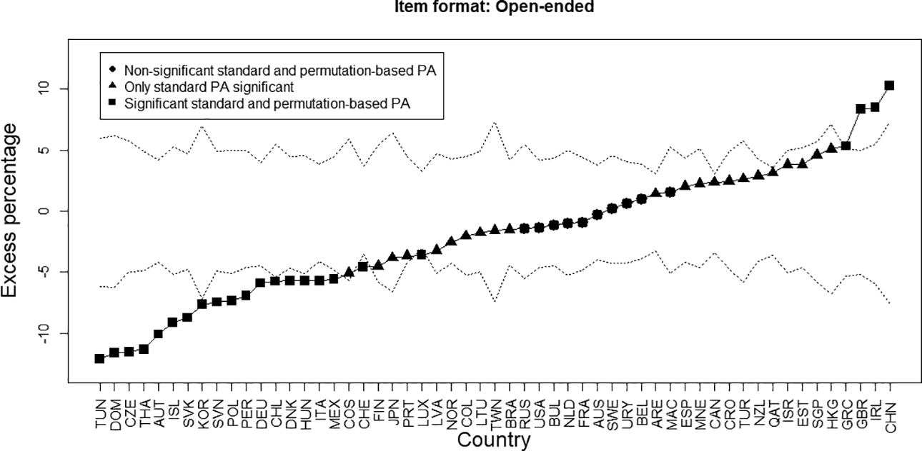
Results of profile analysis for open-ended versus other items in all countries: The solid line indicates the observed excess percentage in the Programme for International Student Assessment data, while the dotted lines are the 2.5th and 97.5th percentiles of the distribution of the excess percentage in the permuted data; the countries are ordered based on the observed excess percentage.
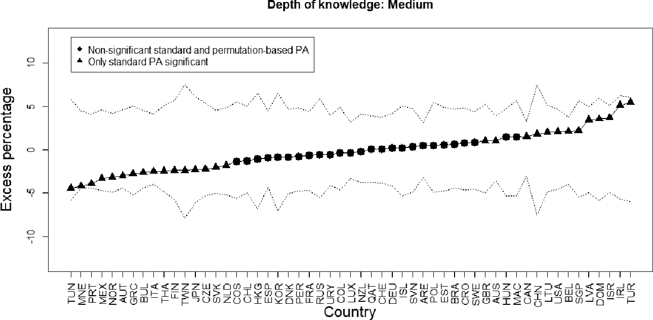
Results of profile analysis for medium depth of knowledge versus other items in all countries: The solid line indicates the observed excess percentage in the Programme for International Student Assessment data, while the dotted lines are the 2.5th and 97.5th percentiles of the distribution of the excess percentage in the permuted data; the countries are ordered based on the observed excess percentage.
Figure 2 shows the results for the items with open response format. As can be observed, in the vast majority of countries (45 of 55), DIF with respect to the open-ended versus nonopen-ended items was found with standard profile analysis, with excess percentages ranging from −12.09 to 10.26. Thus, while in Tunisia, the percentage of students performing better than expected on open-ended questions was 12.09 percentage points lower than expected; in China, this percentage was 10.26 percentage points higher than expected. Figure 2 shows that these test-level results do not generalize to the population level for all 45 countries. Rather, results are generalizable in 23 countries, where the estimated excess percentage falls outside of the confidence bounds (i.e., only for these countries, the results are significant according to the permutation-based profile analysis). 3 For all countries where the excess percentage falls below the confidence band, there is generalizable evidence that they perform better on open-ended questions than expected based on the international results. For all countries where the excess percentage falls above the confidence band, we have evidence that students find open-ended questions easier than expected based on the international results. Thus, for these countries there is evidence—also for the application of future tests—that their overall test results will benefit or suffer from including more open-ended questions on the test. This conclusion does not extend to countries, where significant results occurred only at the test level.
Figure 3 shows the results for the items with medium depth of knowledge. Here, for all countries, the observed excess percentage lies within the 95% bounds of the distribution obtained based on the 1,000 permuted data sets. That is, in no country is the excess percentage for the item feature extreme compared to expectation when the test is randomly split into two sets with 112 and 63 items each. Thus, while at the test level, there are some countries that show better (or worse) performance than expected on the medium depth of knowledge items, there is no reason to expect that these findings would persist for a different set of items than the ones that were on the test. These results therefore do not suggest that certain countries would benefit from (or be adversely affected by) the inclusion of a larger proportion of medium depth of knowledge items on future tests.
5. Simulation Study
5.1. Method
To evaluate the performance of the permutation test in terms of Type I error and power, we conducted a simulation study. Here, we define Type I error as the probability of finding item-feature-related DIF, where none exists and power as the probability of finding item-feature-related DIF where it does exist. Generating parameters for the study are grounded in the results from our empirical analysis. First, we use empirically estimated international item parameters as described previously. This resulted in 175 items with difficulty and discrimination parameters assumed to be equivalent across our simulated countries to begin. These items were assigned to blocks and booklets that matched the PISA 2015 design. Then, to introduce DIF, we used empirical estimates in an analysis, where difficulty parameters were freely estimated across the 55 PISA countries. Specifically, we fitted country-specific models to each country’s data with discrimination parameters fixed to be equal to their international values, but difficulty parameters freely estimated. We computed DIF values for each country
We used empirical sample sizes and achievement distributions as population parameters, with exceptions that we describe next. To exert some control over the study conditions and to examine whether sample size and population-test alignment are factors that influence the results, we replaced 12 empirical countries with generated countries according to the following structure: Two countries each with a combination of three sample sizes (
Type I error of profile analysis was studied under two different conditions. First, we considered a condition where there is no DIF for any item in any country. Second, we considered the possibility of DIF occurring, but not because of item features. In this condition, we generated DIF values for all items in the 12 generated countries by sampling them from
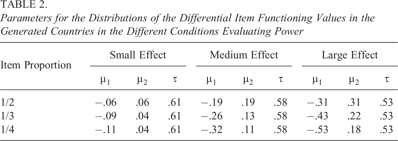
To evaluate whether performance of profile analysis is effected by the proportions of items with an item feature, we considered three different (arbitrary) item features that were assigned to items in three proportions:
Parameters for the Distributions of the Differential Item Functioning Values in the Generated Countries in the Different Conditions Evaluating Power
In the no-DIF condition, 1,000 data sets were generated, in which first the student abilities in each country were sampled from their population distribution and then, using the international item parameters, their responses to the items from the assigned booklets were generated. A measurement invariance multigroup IRT model was fitted to the simulated data as in the empirical example and the estimates of the international item parameters were obtained. Profile analysis with and without the permutation test (with 1,000 replications) was performed for the three item features variables in the six of the generated countries (one for each combination of sample size and population-test alignment). Permutations were performed for each item feature with different item proportions separately, which resulted in 18 permutation-based distributions of the
In the DIF-unrelated-to-item-features condition, the data were generated analogously to the no-DIF condition with the exception that in the 12 generated countries, DIF values randomly sampled for each data set were added to the international item difficulties. Profile analysis was performed in each of the 1,000 simulated data sets and the Type I error was calculated in the same way as in the previous condition. We note that although we use the term “Type I error” for the standard profile analysis, the null hypothesis of this test is not necessarily true in this condition, as the test is for the concrete set of items with an item feature rather than the population of items. Therefore, here we do not expect this test to have the Type I error rate of .05.
Finally, we evaluated the power of the profile for detecting item-feature-related DIF. The data were generated in a similar way as in the DIF-unrelated-to-item-features condition, but the DIF values were generated to be correlated with one of the three item feature variables as described previously. Profile analysis was performed in each of the 9,000 simulated data sets (1,000 for each combination of effect size and proportion of items with the item feature). Power was calculated in similar to the Type I error in the previous two conditions.
5.2. Results
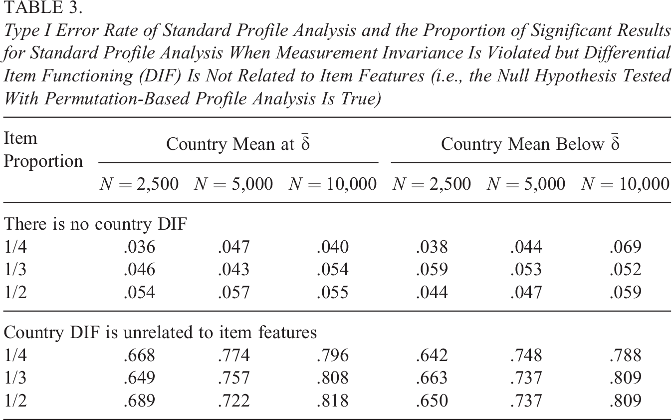
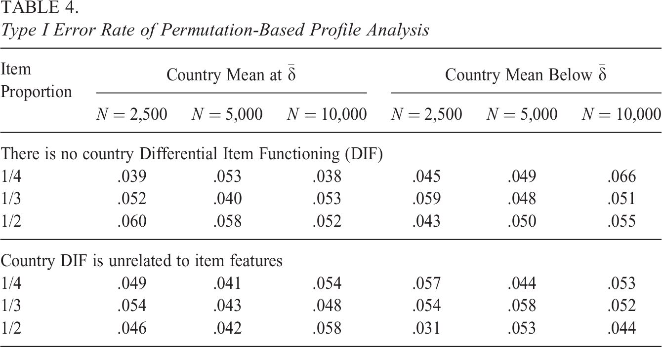
Table 3 shows the results in terms of Type I error for standard profile analysis. When the null hypothesis is true (i.e., there is no country DIF), then the proportion of significant results is close to the nominal value of .05 in all conditions. When measurement invariance is violated but DIF is not related to item features, then for a large proportion of replications, significant results are obtained (.737 on average across conditions, see Table 3). Note that the latter results cannot be interpreted as Type I error since the null hypothesis of standard profile analysis which is aimed at inferences at the test level is violated. The expected value of the difference between the average DIF value of the items with the feature and the average DIF value of the items without the feature is zero, but the probability of it being equal to exactly zero in the sample of 175 test items is negligible. Due to the data generating process, at the test level, there will always be at least some item-feature-related DIF (e.g., in the condition with the item proportion of 1/2, the expected absolute value of the difference between the average DIF values is 0.073), and it is a question of power whether this will can be detected. Because we are looking at averages, the power will be higher than when detecting DIF on the level of individual items. In the case of applications like PISA where sample sizes are large, it is possible to detect even small differences, which is reflected in the large proportion of significant results when DIF is present but not related to item features. As can be seen in Table 3, sample size has a clear effect on this proportion. It is important to note that the overall magnitude of DIF that we used in the simulation was based on what we found in the empirical PISA data. Smaller/larger DIF would lead to smaller/larger percentage of significant results. These results clearly indicate that while standard profile analysis correctly identifies that DIF is present for the sets of items, it cannot be used for making inferences that extend beyond the specific test considered (i.e., about the item feature effect rather than about differences between the two concrete sets of items), as it very often rejects the null hypothesis when violations of measurement invariance are not actually related to item features on the population level. Table 4 shows the results for Type I error for permutation-based profile analysis. Here, both when measurement invariance holds and when country DIF is present, but is not related to item features, Type I error is close to the nominal value of .05.
Type I Error Rate of Standard Profile Analysis and the Proportion of Significant Results for Standard Profile Analysis When Measurement Invariance Is Violated but Differential Item Functioning (DIF) Is Not Related to Item Features (i.e., the Null Hypothesis Tested With Permutation-Based Profile Analysis Is True)
Type I Error Rate of Permutation-Based Profile Analysis
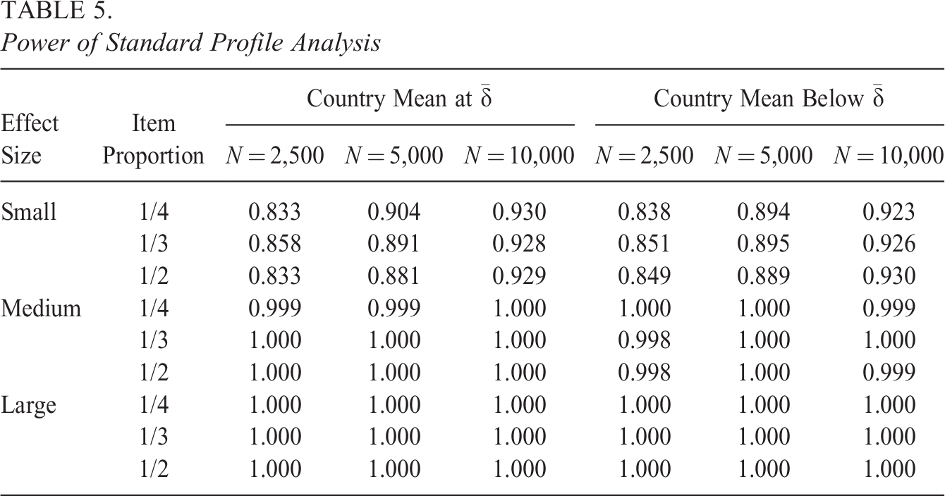
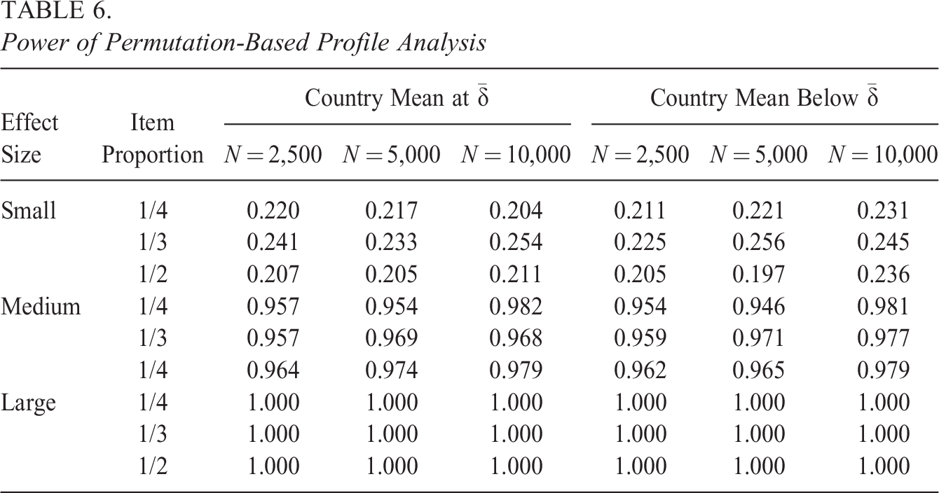
Tables 5 and 6 show power for standard profile analysis and permutation-based profile analysis, respectively. Power is generally higher for standard profile analysis (in all conditions higher than .8), which makes sense since it tests a stricter null hypothesis (and had a very high false positive rate when DIF unrelated to the item features was present, as was seen in Table 3). The power of permutation-based profile analysis is larger than .9 for medium and large correlations (on average .967 and 1.000, respectively) between the item feature and DIF parameters, but relatively low for the small effect (on average .223 across conditions). Low power for the small effect is to be expected since, with only 175 items, high power would not be achieved even if the DIF parameters were known rather than estimated with uncertainty and the effect of the item feature was tested simply by testing the significance of the point-biserial correlation between these parameters and the item feature. For example, when 1/2 of the items have the item feature and the effect of item feature is small, the power of the point-biserial correlation test is .234.
5
Sample size (average power is .726 for N = 2,500, .728 for N = 5,000, and .728 for N = 10,000), proportion of items with the item feature (average power is .727 for 1/4, .736 for 1/3, and .727 for 1/2), and alignment between the country mean and the items’ difficulty (average power is .729 for country mean at
Power of Standard Profile Analysis
Power of Permutation-Based Profile Analysis
6. Discussion
Investigating measurement invariance and violations of it in relation to item features is important as it can bring insights into how educational systems differ from each other internationally, across cultures. Similarly, measurement invariance is important at the national level for understanding how policy-relevant subgroups differ. In the current article, we proposed an extension of profile analysis that allows its application to the 2PL model, as well as allowing for inferences that generalize to the population of items, and hence to future test applications. By extending it to the 2PL model, profile analysis is more flexible. This is important because using the more restrictive model can potentially lead to confounding when the discrimination parameters actually vary across items, a situation that may occur frequently in practice. This extension should thus make profile analysis more relevant for operational settings, where the restrictions imposed by the Rasch model may not always be considered acceptable.
The second contribution of this article was the inclusion of a permutation test aimed at evaluating whether detected measurement invariance violations in profile analysis with the standard
The proposed permutation-based profile analysis allows users to examine whether results found at the test level can be attributed to particular item features and hence can be generalized to the population of items, rather than only being applicable to the idiosyncratic set of items that were included in the specific test administration. Currently, this level of generalizability is not possible in standard profile analysis. Importantly, such generalizability is valuable when evaluating the fairness of future tests that will be administered to participating countries, as it will allow one to determine whether including items with certain feature is likely to positively or negatively impact the performance of particular countries. The results of our empirical analysis and the simulation study show that basing this assessment on the results of a standard profile analysis
Understanding that an item feature explains DIF for certain countries can have notable implications for the fairness of country comparisons. Ideally, country comparisons should not depend on the proportion of items included in the test with a specific feature. When a certain item feature is found to have an effect—as was the case for all but one of the features considered in the illustrative example—this raises the question to what extent a comparison of the performance of countries is affected by the design choices of the test. Would the results have looked differently if more items of a certain type were included in the test? How robust are the rankings of countries to different choices for the test composition? These are questions that require one to consider the population of items, rather than just the set of items that were included in the test, and hence require a test for generalizability such as the permutation test proposed in this article. In this sense, the proposed method should facilitate the evaluation of the robustness of ILSA country comparisons to different choices for the test design.
It may be noted that for the test-level analysis of item-feature effects, the main challenge is to obtain sufficient observations per item; however, obtaining sufficiently high power for detecting item-feature effects that generalize outside the test setting also depends heavily on the number of considered items that do and do not have the feature. Thus, even with the sample sizes usually encountered in ILSAs, one may have trouble gaining sufficient power to study the effect of each item feature, especially if a certain feature is only shared by a small subset of the items on the test. In this context, it may be relevant to note that the absence of evidence of an effect of a certain item feature should not be taken as conclusive evidence for the actual absence of an effect, especially when there were not that many items on the test that shared the considered feature.
In this article, we have taken profile analysis as the starting point for developing a procedure for investigating item-feature-related DIF in a generalizable way. However, the kind of permutation test that we proposed can be adapted to other measures of item-feature-related DIF that do not yet address the issue of generalizability, like differential facet functioning and differential bundle functioning. In both cases, the distribution of the DIF-statistic used to quantify DIF for the group of items can be obtained using permutations of items into random subsets and inferences can be made based on how the observed statistic relates to this distribution.
One limitation of the proposed procedure is that item features are evaluated independently of each other and it is not possible to evaluate the effect of one item feature after controlling for other item features. As such, caution should be taken when interpreting the results, especially when item features are correlated with each other.
When testing the effects of multiple item features in multiple countries, researchers should be aware of the effects of multiple testing on the overall Type I error of the procedure. This problem, however, is not specific to the developed permutation-based profile analysis but applies to any method aimed at testing the effects of multiple item features on DIF in multiple groups (e.g., differential facet functioning and differential bundle functioning). Depending on the level at which the inferences are being made (country level, test level, item-feature level), multiple testing corrections can be applied at the corresponding level. As many of these methods (Bonferroni, 1936; Hochberg, 1988; Holm, 1979; Šidák, 1967) involve decreasing the
Another limitation is that currently the permutation-based profile analysis can be used only for binary categorizations of the items (e.g., open-ended items vs. multiple-choice items). Permutation-based profile analysis can be extended to allow for multiple item categories similar to how it has been done for standard profile analysis (Verhelst, 2012), but this goes beyond the scope of the current article. If the item feature is not categorical, but continuous (e.g., some measure of item complexity), then to use our procedure, it has to be discretized, which would lead to some loss of information.
A further area for future research is to investigate whether adjusting the international scaling model to account for known, generalizable item-feature-related DIF would produce desirable outcomes. One possibility could be to include country-specific item parameters for items with features known to function differently in particular countries. A second option could be to use a linear logistic test model with
Footnotes
Declaration of Conflicting Interests
The author(s) declared no potential conflicts of interest with respect to the research, authorship, and/or publication of this article.
Funding
The author(s) received no financial support for the research, authorship, and/or publication of this article.