Sage Journals: Discover world-class research

Abstract

One of the primary goals of international large-scale assessments in education is the comparison of country means in student achievement. This article introduces a framework for discussing differential item functioning (DIF) for such mean comparisons. We compare three different linking methods: concurrent scaling based on full invariance, concurrent scaling based on partial invariance using the RMSD statistic, and robust and nonrobust linking approaches based on separate scaling. Furthermore, we analytically derive the bias in the country means of different linking methods in the presence of DIF. In a simulation study, we show that the partial invariance and robust linking approaches provide less biased country means than the full invariance approach in the case of biased items.

Keywords

linking differential item functioning RMSD statistic partial invariance international large-scale assessments

One major goal of large-scale assessment studies in education is to compare cognitive outcomes across many groups. For example, the Program for International Student Assessment (PISA; Organization for Economic Cooperation and Development [OECD], 2017) and the Program for the International Assessment of Adult Competencies (PIAAC; Yamamoto et al., 2013) provide international comparisons of student performance and adult skills for large groups of countries (72 countries in PISA 2015; 38 countries in PIAAC). A major methodological challenge of these comparisons is that the items of the achievement tests show differential item functioning (DIF) in specific countries. Uniform DIF is present if an item is relatively easier or more difficult in a specific country than at the international level (Holland & Wainer, 1993; Penfield & Camilli, 2007). In this case, an item parameter is noninvariant across countries. It has been argued that country DIF has the potential to bias the estimation of country-specific means and standard deviations (Kankaras & Moors, 2014).

In general, three different approaches for conducting cross-national comparisons in the presence of DIF can be distinguished between. First, in the concurrent scaling approach under full invariance, DIF effects are completely ignored, and common item parameters are estimated in a multiple-group item response theory (IRT) model. In this approach, country-specific item parameters are treated as completely invariant across groups when estimating country-specific means and standard deviations. Second, in the concurrent scaling approach under partial invariance, items with noninvariant parameters across countries are identified using country-specific item fit statistics and cutoff values as screening criteria. Based on this screening process, country-specific means and standard deviations are estimated in a multiple-group IRT model in which the parameters of items with no country DIF are constrained to be equal across countries, and the parameters of items with country DIF are allowed to be country-specific. As a third approach, we consider an approach that combines a separate scaling approach with linking methods. In contrast to the concurrent scaling approaches, item parameters are calibrated separately for each country, and no invariance assumptions are made for the group-specific item parameters. In the next step, the group-specific ability distributions are obtained by applying a linking method that places the group-specific item parameters onto a common metric. We extend the linking procedures of Haberman (2009) and Haebara (1980) to the case of many groups and robust linking functions. Robust linking functions have the desirable property that items with large DIF effects are treated as outliers that do not impact country mean comparisons. However, in contrast to concurrent scaling under partial invariance, which removes items with large DIF effects from country comparisons, robust linking methods do not rely on DIF statistics and allow for more principled modeling of DIF effects.

This article is organized as follows. First, we discuss the role that uniform DIF plays in group comparisons in the two-parameter logistic (2PL) model. We argue that it is crucial to differentiate between two group-specific item sets: so-called reference items and biased items. Reference items are group-specific items that allow valid group comparisons. Biased items have DIF effects that have the potential to distort group comparisons. Then, we discuss three different approaches for comparing country means in the presence of DIF: concurrent scaling under full invariance, concurrent scaling under partial invariance, and linking based on separate scaling. We show analytically that these approaches place different constraints on the DIF effects of reference items and biased items. We present the results of a simulation study, which investigated the performance of the different scaling approaches under different conditions for the DIF effects of reference and biased items. Finally, we illustrate the different approaches by reanalyzing the reading domain data of the PISA 2006 assessment.

Uniform DIF in the 2PL Model

In the following, the concept of DIF (Holland & Wainer, 1993; Millsap, 2011) for multiple groups (e.g., countries in large-scale assessments) is discussed. For G groups (g = 1,…, G), items i = 1,…, I are administered. It is assumed that a unidimensional item response model holds in each group with group-specific item response functions (IRF) P_ig(θ), indicating the probability of a correct item response conditional on ability θ. According to Mellenbergh (1989; see also Millsap, 2011), there is no DIF for item i (i.e., item i is measurement invariant across groups) if a common IRF P_i(θ) exists so that

P_{i} (θ) \equiv P_{i 1} (θ) = P_{i 2} (θ) = \dots = P_{i G} (θ) for all values of θ .

To check whether there is DIF for item i, the ability θ (or its distribution) has to be known in Equation 1. However, this is rarely the case in practice, and item parameters are needed to estimate the ability. This illustrates the circularity in the DIF definition (Camilli, 1993) and highlights that DIF can only be identified at the level of single items if additional assumptions are made.

The IRF in the 2PL model (Birnbaum, 1968) is given as

P_{i g} (θ) = Ψ (a_{i} (θ - b_{i} - e_{i g})), θ \sim N (μ_{g}, σ_{g}^{2}),

where b_i is the common item difficulty for item i and e_ig are group-specific item difficulty deviations with nonzero values indicating uniform DIF; Ψ denotes the logistic distribution function, and it is assumed that the abilities are normally distributed in group g. The one-parameter logistic (1PL) model arises if item discriminations a_i are set to 1 in Equation 2. It has been demonstrated that the 1PL model is not identified. Identification constraints among item parameters are needed to estimate the means µ _g and the standard deviations σ _g of the ability distributions for the G groups and the DIF effects e_ig (Bechger & Maris, 2015; Robitzsch & Lüdtke, 2020; Soares et al., 2009). The same principle of nonidentification also applies to the case of uniform DIF in the 2PL model. This can be seen by reparametrizing Equation 2 as follows:

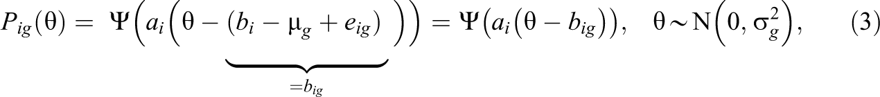
P_{i g} (θ) = Ψ (a_{i} (θ - \underset{\underset{= b_{i g}}{︸}}{(b_{i} - μ_{g} + e_{i g})})) = Ψ (a_{i} (θ - b_{i g})), θ \sim N (0, σ_{g}^{2}),

where the group-specific item parameters b_ig are identified without additional constraints and are composed of the common item difficulties b_i of item i, the means of the ability distributions µ _g , and the uniform DIF effects e_ig. One possible identification constraint is to set the standard deviation $σ_{1}$ of the first group to one, while identifying the standard deviations $σ_{g}$ of groups g = 2,…, G. Furthermore, given the $I \cdot G$ group-specific item parameters b_ig, further constraints on the $I \cdot G$ DIF effects $e_{i g}$ are needed to identify the G group means µ _g . To resolve the identification issue, the set of items for each group is partitioned into two distinct sets (see Robitzsch & Lüdtke, 2020, for the case of the 1PL model). More specifically, we assume that for each group g a subset of reference items $J_{R, g} \subset J = \{1, \dots, I\}$ exists so that $\sum_{i \in J_{R, g}} e_{i g} = 0$ for g = 1,…, G. Items in the set $J_{R, g}$ serve as the reference for defining the scale for group g, which resolves the identification issue.¹ The group-specific set of biased items is then defined as $J_{B, g} = J \ J_{R, g}$ . Biased items have the potential to bias group mean estimates because the uniform DIF effects of biased items can differ from zero on average, that is, $\sum_{i \in J_{B, g}} e_{i g} \neq 0$ . It is important to emphasize that in our definition, all items are allowed to have DIF (i.e., DIF items). In large part of the DIF literature and most simulation studies (e.g., Kopf et al., 2015), it is assumed that for each group g, there is a set of anchor items $J_{A, g} \subset J = \{1, \dots, I\}$ so that $e_{i g} = 0$ for all $i \in J_{A, g}$ and g = 1,…,G. If the DIF effects e_ig of reference items are chosen to be “small” (or even 0) compared to the DIF effects of biased items, it is plausible to consider the DIF effects of biased items as outliers (He et al., 2013; Magis & De Boeck, 2011).

In the following, we denote a test to have balanced DIF if the DIF effects sum to zero for all groups (within each group g), that is, $\sum_{i \in J} e_{i g} = 0$ . Because the DIF effects of reference items sum to zero by definition, balanced DIF is equivalent to the condition that the DIF effects of biased items sum to zero (i.e., $\sum_{i \in J_{B, g}} e_{i g} = 0$ for g = 1,…,G).² A test has unbalanced DIF if at least one group g exists for which $\sum_{i \in J_{B, g}} e_{i g} \neq 0$ holds. One central argument in the DIF literature is that items with DIF effects have the potential to bias the estimated group means and should, therefore, not be included in group comparisons (e.g., OECD, 2017, for arguments in the PISA study, or Kopf et al., 2015). Biased estimates of group means can be expected, particularly in the case of unbalanced DIF.³

By distinguishing between reference items and biased items, we highlight the vital role that identification constraints play in estimating the means of the group-specific ability distribution. However, at a more conceptual level, it needs to be emphasized that the decision about whether an item with a DIF effect is classified as a reference item or as a biased item should not be based solely on statistical criteria (see Camilli, 1993; Gomez-Benito et al., 2018; Penfield & Camilli, 2007; Zwitser et al., 2017, for this argument). More specifically, the identification of a mean for group g relies only on items from the set of reference items $J_{R, g}$ and does not rely on the set $J_{B, g}$ of biased items. Consequently, basing the decision to remove items from the reference item set exclusively on statistical criteria could result in construct underrepresentation (i.e., removing items with DIF effects that are construct relevant; see Camilli, 1993; Penfield & Camilli, 2007). If a researcher is confident that all items in the test are construct relevant, no items with DIF effects should be removed from linking. Hence, all items serve as reference items and an identification constraint (i.e., $\sum_{i \in J} e_{i g} = 0$ ) has to be assumed. Camilli (1993) pointed out that DIF detection procedures should be accompanied by expert reviews of items showing DIF. Only those items should be removed from group comparisons for which it is defensible to argue that DIF was caused by construct irrelevant factors.

It is instructive to relate our definitions of DIF to the terminology of the measurement invariance literature (Meredith, 1993; Vandenberg & Lance, 2000) and to distinguish between the following scenarios of DIF effects. If there are no biased items in all groups and e_ig = 0 for all items in all groups, there are no DIF effects. This situation is labeled as full invariance. The situation in which there is a set of anchor items in each group (e.g., a subset of items is DIF-free) is labeled as partial invariance (Byrne et al., 1989). It is typically assumed that DIF effects are sparsely distributed (Liang & Jacobucci, 2020); that is, only a minority of items have DIF effects. The situation in which all items have DIF effects is denoted as complete noninvariance. Furthermore, the particular case in which all items serve as reference items (i.e., $J_{R, g} = J$ and $\sum_{i \in J} e_{i g} = 0$ for all groups g) bears similarity with the definition of approximate invariance (Byrne & van de Vijver, 2017; van de Schoot et al., 2013). However, in approximate invariance, one additionally assumes that DIF effects e_ig are modeled with a centered normal distribution N(0,ν²). The variance ν² of DIF effects can be fixed (e.g., ν² = 0.001 or ν² = 0.01; see van de Schoot et al., 2013), estimated (Fox & Verhagen, 2010; Verhagen et al., 2016). Alternatively, DIF effects can be parameterized as residual covariances (Fox et al., 2017, 2020). Finally, the situation in our definition that involves both reference items and biased items is similar to partial approximate invariance (van de Schoot et al., 2013). In this case, the DIF effects of reference items are modeled with a centered normal distribution N(0, ν²), and biased items have DIF effects that do not sum to zero.

Scaling Approaches for Multiple-Group Comparisons

In the following, we discuss different approaches for comparing group means in the presence of uniform DIF in the 2PL model. We distinguish between three scaling strategies that differ concerning the degree of invariance they assume for the item parameters. First, we discuss concurrent scaling approaches that assume full invariance of item parameters across groups. In this approach, DIF effects are ignored and not modeled (i.e., DIF effects e_ig are not included as parameters in the statistical model) when estimating group-specific means and standard deviations. Second, we discuss concurrent scaling approaches that assume partial invariance. In this approach, group-specific item parameters only need to be included for a subset of DIF effects (von Davier et al., 2019). Typically, the set of items with modeled DIF effects—which is aimed to match the set of biased items—is allowed to vary from group to group, and a DIF statistic is required to determine the set of biased items for each group. Third, we propose a separate scaling approach that employs linking methods and does not pose invariance assumptions on item parameters (complete noninvariance). All DIF effects are allowed in this approach, and group-specific means and standard deviations are estimated under different types of linking functions.

Concurrent Scaling Under Full Invariance

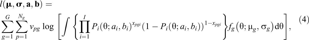
In concurrent scaling under the assumption of full invariance of item parameters, maximum likelihood (ML) estimation is used to estimate a multiple-group item response model that does not include any DIF effects. More specifically, the following log-likelihood function is maximized with respect to the unknown model parameters $(μ, σ, a, b)$ for the item responses $x_{p g}$ of persons p = 1,…, N_g in groups g = 1,…, G:

l (μ, σ, a, b) = \sum_{g = 1}^{G} \sum_{p = 1}^{N_{g}} v_{p g} log [\int \{\prod_{i = 1}^{I} P_{i} {(θ; a_{i}, b_{i})}^{x_{p g i}} {(1 - P_{i} (θ; a_{i}, b_{i}))}^{1 - x_{p g i}}\} f_{g} (θ; μ_{g}, σ_{g}) dθ],

where the ability θ in group g is assumed to be normally distributed (i.e., $θ \sim N (μ_{g}, σ_{g}^{2})$ ), and all group means and standard deviations are collected in vectors $μ$ and $σ$ , respectively (marginal maximum likelihood estimation, MML; von Davier & Sinharay, 2014). In addition, invariant item parameters a and b across groups are assumed, and the IRF are given as $P_{i} (θ; a_{i}, b_{i}) = Ψ (a_{i} (θ - b_{i}))$ . The concurrent scaling approach under full invariance allows the estimation of all common item parameters as well as country-specific means and standard deviations in one step. In the log-likelihood function in Equation 4, sampling weights v_pg are included in international large-scale assessment (ILSA).

If the item response model is correctly specified, the ML estimator is consistent (White, 1982). However, the model in Equation 4 is misspecified because the true IRF $P_{i g} (θ) = Ψ (a_{i} (θ - b_{i} - e_{i g}))$ involve unique group-specific DIF effects, which are ignored in concurrent scaling under full invariance. For misspecified models, the ML estimator $(\hat{μ}, \hat{σ}, \hat{a}, \hat{b})$ is still consistent and converges to the maximizer of the Kullback–Leibler information (White, 1982; see also Kuha & Moustaki, 2015). Ignoring DIF effects in the estimation of Equation 4 provides estimates of the group-specific distribution parameters that are the best approximation with respect to the Kullback–Leibler information. Because the model is misspecified, model-robust standard errors (also known as sandwich standard errors; White, 1982) have to be used to obtain valid statistical inference. Given true data-generating parameters $(μ, σ, a, b, e)$ , the ML estimator $(\hat{μ}, \hat{σ}, \hat{a}, \hat{b})$ will typically be biased, even in large samples. Nevertheless, we can derive $\hat{μ}$ as a function of the data-generating parameters (see Kolenikov, 2011, for a similar technique; see Robitzsch & Lüdtke, 2020). In infinite sample sizes, the estimated group mean ${\hat{μ}}_{g}$ is a biased estimator of the true group mean $μ_{g}$ because of the existence of DIF effects. In Appendix A, we apply a Taylor approximation of the likelihood function around DIF effects to obtain a bias approximation. The derivation rests on the assumption that joint item parameters are consistently estimated, that is, $\hat{a} = a$ and $\hat{b} = b$ . In large sample sizes, the bias of the estimator of the group mean ${\hat{μ}}_{g}$ can be approximately written as a weighted combination of the DIF effects e_ig (Appendix A, Equation A7):

{\hat{μ}}_{g} ≃ μ_{g} - \sum_{i = 1}^{I} w_{i g} e_{i g},

where the weights $w_{i g} = w_{i g} (μ_{g}, σ_{g}, a_{i}, b_{i})$ in the ML estimation are primarily driven by the item information functions, and it holds that $\sum_{i = 1}^{I} w_{i g} = 1$ in each group g. As the IRF of items with more extreme difficulties is less precisely estimated, the DIF effects of extreme difficulties are down-weighted in Equation 5. Therefore, the bias of a group mean is primarily caused by items for which DIF effects $e_{i g}$ are large, and their item difficulties are located close to the center of the distribution, that is, $|μ_{g} - b_{i}|$ is small. Overall, the concurrent scaling approach under full invariance with fixed items only provides unbiased estimates if the constraint $\sum_{i = 1}^{I} w_{i g} e_{i g} = 0$ is fulfilled in the data-generating model.

Concurrent Scaling Under Partial Invariance Using DIF Statistics

In contrast to concurrent scaling under full invariance that ignores DIF effects, concurrent scaling under partial invariance allows some of the item parameters with large DIF effects to vary across groups. In this approach, country comparisons are based on a multiple-group IRT model in which, for some of the items, item-by-group interactions are specified (Oliveri & von Davier, 2011; von Davier et al., 2019). The decision about which item parameters obtain group-specific item parameters is based on test statistics for DIF (see Penfield & Camilli, 2007, for an overview). The goal is to determine the set of biased items $J_{B, g}$ for each group that obtain group-specific item parameters while the DIF effects in the set of reference items $J_{R, g}$ are set to zero. More detailedly, a DIF statistic T_ig of interest is selected, and item i for group g is declared to be in the DIF item set $J_{DIF, g}$ if |T_ig| > c for a cutoff value c. A partial invariance approach typically consists of two steps (e.g., von Davier et al., 2019). In the first step, a multiple-group IRT model is estimated under the assumption of full invariance to obtain estimates for the country means and standard deviations as well as for the common item parameters $(μ, σ, a, b)$ . Based on these estimated parameters, the DIF statistic T_ig is computed for every item in every group. In the second step, a multiple-group IRT model is estimated in which DIF effects e_ig are freely estimated if the item i belongs to the DIF item set $J_{DIF, g}$ in group g. From this model, parameter estimates for $(μ, σ, a, b, e)$ are obtained where only a subset of DIF effects $e$ differs from zero. Similarly to the derivation of the full invariance approach (and assuming that common item parameters a and b can be consistently estimated), the estimated group means in the partial invariance approach can be determined as

{\hat{μ}}_{g} ≃ μ_{g} - \sum_{i \in J ∖ J_{DIF, g}}^{​} w_{i g} e_{i g},

where w_ig are precision weights. If the DIF item set $J_{DIF, g}$ coincides with the set of biased items $J_{B, g}$ , the weighting of DIF effects in Equation 6 is conducted on the reference item set $J_{R, g}$ . It can be expected that the partial invariance approach can provide approximately unbiased group means if the set of biased items is correctly detected by the test statistic T_ig. If the reference items do not have DIF effects, the partial invariance approach provides unbiased group mean estimates.

Many DIF statistics have been proposed in the literature (see Penfield & Camilli, 2007, for an overview). In the following, we use the root mean squared deviation (RMSD) statistic (see Tijmstra et al., 2020), which is now in operation in the ILSA PISA (OECD, 2017; von Davier et al., 2019) and PIAAC (Yamamoto et al., 2013). The RMSD for an item i in country g assesses the distance between a group-specific IRF $P_{i g}$ and a reference IRF P_i (which does not include group-specific item parameters):

{RMSD}_{i g} = \sqrt{\int {(P_{i g} (θ) - P_{i} (θ))}^{2} f_{g} (θ) dθ}

where f_g denotes the density of the ability distribution in group g. It should be noted that the RMSD statistic also appears in the literature as the RISE statistic (Sueiro & Abad, 2011) for assessing item misfit. The IRF in Equation 7 involve the unknown functions $P_{i g} (θ)$ , $P_{i} (θ)$ , and $f_{g} (θ)$ , which need to be replaced with sample-based analogs. The computation is based on a fitted multiple-group 2PL model that assumes fully invariant item parameters (for estimation details, see Köhler et al., 2020;Tijmstra et al., 2020).

Several benchmarks for interpreting DIF effects as large have been proposed for the RMSD statistic for the 1PL or the 2PL model: .055 (Buchholz & Hartig, 2019), .08 (Köhler et al., 2020), .10 (Oliveri & von Davier, 2011), .12 (OECD, 2017, p. 151), .15 (OECD, 2017, p. 174; von Davier et al., 2019), and .20 (OECD, 2015, p. 30). A recent simulation study for the 1PL model suggested that cutoff values of .05 or .08 are to be preferred to .12 (Robitzsch & Lüdtke, 2020). Notably, the RMSD statistic typically increases in smaller sample sizes, making it difficult to apply rules of thumb independent of sample size (Köhler et al., 2020). In small to moderate sample sizes, the detection of DIF items based on statistical significance tests might be preferable (Battauz, 2019; Magis et al., 2010; Millsap, 2011). Overall, the specification of an appropriate cutoff value to identify items with DIF effects is a challenging aspect in applying the partial invariance approach.

Linking With Separate Scaling Under Full Noninvariance

In the third approach, no invariance assumptions are made for the group-specific item parameters. In this approach, group comparisons are based on a two-step procedure that employs linking methods (see Kolen & Brennan, 2014) based on item parameters from a separate scaling within groups. In the first step, a 2PL model is fitted separately for each group (assuming $θ \sim N (0, 1)$ ), resulting in item parameter estimates ( ${\hat{a}}_{g}, {\hat{b}}_{g})$ (g = 1,…, G). Hence, item parameters are allowed to vary across groups. In the second step, the parameters of the group-specific ability distributions (i.e., group means µ _g and standard deviations σ _g ) are estimated by applying a linking method in order to place the group-specific item parameters onto a common metric (Battauz, 2017). In the following, we discuss the Haberman and the Haebara linking methods suited for linking multiple groups.

Haberman linking

In Haberman linking, the group-specific item parameters a_ig and b_ig are used to simultaneously estimate common item parameters b_i, group means µ _g , and standard deviations σ _g . Haberman (2009) proposed a regression approach to estimate group means µ, standard deviations σ, and common item parameters a and b by applying two regression models for item parameters. The estimation of σ and a is conducted by specifying a linear regression model for logarithmized item loadings. In more detail, for the first regression model, the following optimization criterion is minimized:

H_{1} (σ, a) = \sum_{g = 1}^{G} \sum_{i = 1}^{I} ρ (log {\hat{a}}_{i g} - log σ_{g} - log a_{i})

where ρ is a loss function (Fox, 2016), and the identification constraint σ₁ = 1 is used. The second regression model for estimating µ and b is based on estimated difficulties ${\hat{b}}_{g}$ and estimated standard deviations $\hat{σ}$ from the first step:

H_{2} (μ, b) = \sum_{g = 1}^{G} \sum_{i = 1}^{I} ρ ({\hat{b}}_{i g} {\hat{σ}}_{g} + μ_{g} - b_{i}),

where the identification constraint µ₁ = 0 is used. It should be emphasized that the regression models (in Equations 8 and 9) correspond to a two-way ANOVA with main effects and that the presence of DIF effects is equivalent to the presence of interaction effects in the two-way ANOVA (Robitzsch & Lüdtke, 2020).

Haberman (2009) proposed the squared loss function $ρ (x) = x^{2}$ , which results in a linear regression model estimated by ordinary least squares (i.e., L₂ regression). As DIF effects can be characterized as outlying observations, robust loss functions should be preferred for the unbiased estimation of parameters in the regression model (Fox, 2016). Here, we apply the median regression (L₁ regression as a special case of quantile regression; see Koenker, 2017), which uses the loss function $ρ (x) = |x|$ . The more general L_p regression loss function $ρ (x) = {|x|}^{p}$ has been investigated in Robitzsch (2020a).

For the quadratic loss function $ρ (x) = x^{2}$ and the absolute value loss function $ρ (x) = |x|$ , the expected value of the group mean estimate ${\hat{μ}}_{g}$ is approximately given in large samples as (see Appendix B, Equation B2):

{\hat{μ}}_{g} ≃ μ_{g} - B_{g}

where the biasing term B_g is given as the mean of the DIF effects e_ig for $ρ (x) = x^{2}$ and the median of e_ig effects for $ρ (x) = |x|$ . Hence, it can be concluded that the median regression is more robust to outlying DIF effects.

Haebara linking

It can be expected that Haberman linking can become unstable in small sample sizes because item parameter estimates can be imprecisely estimated. However, estimates of IRF can be quite stable even for unstable item parameters (Ogasawara, 2002). The Haebara linking method relies on linking IRF across groups (Kolen & Brennan, 2014) and can provide more stable group mean estimates than Haberman linking. A generalization of Haebara linking to multiple groups minimizes the summed distances of group-specific IRF and a reference IRF (see Arai & Mayekawa, 2011). More formally, the following criterion is minimized:

H (μ, σ, a, b) = \sum_{g = 1}^{G} \sum_{i = 1}^{I} \int ρ (Ψ ({\hat{a}}_{i g} [θ - {\hat{b}}_{i g}]) - Ψ (a_{i} [σ_{g} θ - b_{i} + μ_{g}])) ω (θ) dθ

where ρ is a loss function, and $ω$ is a weighting function. Haebara (1980) proposed a quadratic loss function $ρ (x) = x^{2}$ . Alternatively, the robust loss functions $ρ (x) = |x|$ (He et al., 2015; He & Cui, 2020) and $ρ (x) = {|x|}^{p}$ ( $p \geq 0$ ; Robitzsch, 2020b) have been proposed for Haebara linking, which are expected to be superior to a quadratic loss function in the presence of DIF effects. The DIF effects are treated as outlying observations in the optimization criterion in Equation 11.

The expected group mean estimate of Haebara linking for the quadratic and the absolute value loss function is of the same form as in Haberman linking (Equation 10; see Appendix C, Equation C4). Each item i in each group g is associated with a weight w_ig that is a function of a_i, b_i, µ _g , and σ _g . For the loss function $ρ (x) = x^{2},$ the biasing term B_g is the weighted mean of DIF effects e_ig using weights w_ig, while for the absolute value function $ρ (x) = |x|$ , the biasing term is given as the weighted median of DIF effects e_ig.

Computation of Standard Errors

The uncertainty in the estimated group means has to be taken into account correctly in statistical inference. In the concurrent scaling approach based on full invariance, standard errors due to the (independent) sampling of persons are readily obtained in ML estimation. Unfortunately, the concurrent scaling approach based on partial invariance does not directly provide valid standard errors because the preliminary step of detecting items with DIF effects is ignored in standard error assessment (Burnham & Anderson, 2002). Standard errors for the linking approaches based on separate scalings rely on the delta formula (Andersson, 2018; Battauz, 2015; Robitzsch, 2020a). The computation of standard errors based on resampling techniques such as balanced repeated replicate weights (used in PISA; OECD, 2009; Kolenikov, 2010) is a viable alternative, particularly in the case of stratified clustered sampling (Andersson, 2018; Battauz, 2017; Haberman et al., 2009). In this article, we are also interested in comparing group mean estimates obtained from different scaling models that were applied to the same sample. Thus, a significance test for a group mean difference evolving from two different models based on the same data set is required because the assumption that the standard errors of the two models are independent is not justified. A simple but effective alternative for computing standard errors consists of applying resampling methods in which the group mean difference between two models is also computed in the replication samples (Burnham & Anderson, 2002; Macaskill, 2008).

Research Questions

The primary research goal of our study is to compare the performance of the linking approach with a separate scaling approach with two concurrent scaling approaches for estimating country means in the presence of uniform country DIF. We expect that the performance of concurrent scaling under partial invariance would depend on the proportion and type of DIF effects of biased items. In the case of balanced DIF (i.e., DIF effects of biased items that sum to zero), efficiency losses of estimated group means are expected when items were removed from country comparisons in concurrent scaling under partial invariance (DeMars, 2020). Furthermore, in this scenario, it could be speculated that concurrent scaling under full invariance and separate scaling with nonrobust linking would be superior to scaling under partial invariance. In the case of unbalanced DIF (i.e., DIF effects of biased items are of the same sign), we expect that robust linking would provide less biased group mean estimates than the full invariance approach and nonrobust linking. The performance of concurrent scaling under partial invariance is expected to strongly depend on selecting an appropriate cutoff value for the RMSD statistic. We also investigate whether the concurrent scaling approaches have some advantages in small samples because they combine information from different groups when estimating item parameters.

Simulation Study

Simulated Conditions

We simulated data from a 2PL model for G = 20 countries. For each country, abilities were normally distributed with mean µ _g and standard deviation σ _g . Across all conditions and replications of the simulation, the country means and standard deviations were held fixed and ranged between −0.92 and 0.81 for means (with an average of 0.00) and between 0.82 and 1.06 for standard deviations (with an average of 0.91). The values were chosen to mimic the typical variability of the country means in a PISA study. The total population containing all students in all countries had a mean of zero and a standard deviation of 1. Country-specific item parameters β _ig were generated according to $β_{i g} = b_{i} + e_{i g}$ , where b_i is the common item parameter, and e_ig is the country-specific uniform DIF effect. Item slopes a_i were held invariant across countries. In total, I = 20 items were used in the simulation. The common item parameters a_i, and b_i ranged between 0.50 and 1.42 (M = 1.00) and between −1.62 and 1.39 (M = 0.00) for item slopes and item difficulties, respectively.⁴

In each country, the sets of biased and reference items were held fixed across conditions and replications with a fixed proportion of biased items. For a fixed proportion $π_{B}$ of biased items, an integer variable Z_ig was defined for each item i in each group g, which had values of 0 (reference item), +1 (biased item with a positive uniform DIF effect), or −1 (biased item with a negative uniform DIF effect). Furthermore, standardized effects ε _ig were specified that were nonzero for reference items and zero for biased items. These effects fulfilled the conditions $\sum_{i = 1}^{I} (1 - | Z_{i g} |) ε_{i g} = 0$ (i.e., DIF effects of reference items sum to zero) and $\sum_{i = 1}^{I} (1 - | Z_{i g} |) ε_{i g}^{2} = I (1 - π_{B})$ (i.e., SD of DIF effects of reference items equals 1). In the case of balanced DIF, DIF effects were computed as $e_{i g} = (|Z_{i g}| - 1) S D_{A} ε_{i g} + Z_{i g} δ$ , where SD_A was the prespecified standard deviation of the DIF effects of the reference items. A small variability of the true item difficulties across groups could be a reasonable assumption in applications (Monseur et al., 2008). In the case of balanced DIF, half of the biased items received a uniform DIF effect of δ and for the other half, the uniform DIF effect was set to −δ. In the case of unbalanced DIF, all biased items within a country received a uniform DIF effect of either δ or −δ. This property was implemented by defining a variable D_g for which 10 countries had the value +1, and the other 10 countries had the value −1. The DIF effects for unbalanced DIF were defined as $e_{i g} = (|Z_{i g}| - 1) S D_{A} ε_{i g} + |Z_{i g}| D_{g} δ$ . All data-generating parameters can be downloaded from https://doi.org/10.17605/OSF.IO/27QDU.

For each condition of the simulation design, 500 replications were generated. More specifically, we manipulated the following four factors in our simulation design to mimic typical situations in large-scale assessment studies: the number of persons per country (N = 250, 500, and 1,000), the proportion of biased items (0%, 10%, and 30%; see Magis & De Boeck, 2011), the standard deviation of the DIF effects of the reference items (SD_A = 0, and .15; see Monseur et al., 2008), and the type of DIF effects of the biased items (balanced vs. unbalanced). The DIF effect size for the biased items was fixed to δ = 0.6, which corresponds to a large DIF effect size (i.e., C-DIF according to the ETS classification; see Penfield & Camilli, 2007).

Analysis Models and Criteria

We used three different scaling strategies to obtain country means in each replication. First, we specified a multiple-group 2PL model with invariant item parameters across countries (concurrent scaling under full invariance; FI). Second, we implemented concurrent scaling under partial invariance using the RMSD statistic (PI-RMSD) in which items in a country with RMSD values larger than .05, .08, or .12 received country-specific item difficulties while still assuming country-invariant item slopes. Third, we used two linking approaches (Haberman method and Haebara method) that do not rely on invariance assumptions for item parameters. In both approaches, a nonrobust version (HAB and HAE) or a robust version (RHAB and RHAE) was used to link the item parameters that were obtained from a separate scaling within each country. For all analyses, the R software (R Core Team, 2020) and the R packages sirt (Robitzsch, 2020c) and TAM (Robitzsch et al., 2020) were used.

In each scaling strategy, for the first country, the mean was set to zero, and the standard deviation was set to 1 to identify all model parameters. For the country comparisons, country means were linearly transformed so that the total population of students across countries had a mean of zero and a standard deviation of 1. We used two criteria to evaluate the performance of the different approaches: average absolute bias and average root mean square error (RMSE) across countries. Average absolute bias was computed by averaging the absolute biases of all country means. Average absolute biases greater than .03 (i.e., about 3 points in the PISA metric) were considered substantial because standard errors of the country means in ILSA are usually about that size (e.g., OECD, 2017). The average RMSE was calculated by averaging the RMSEs across countries.

Results

Table 1.

Average Absolute Bias (Bias) and Average Root Mean Square Error (RMSE) of Group Means as a Function of Proportion of DIF Items, and Standard Deviation of DIF Effects of Reference Items for a Sample Size of N = 1,000 and for Balanced DIF and Unbalanced DIF

			PI-RMSD
%BI	SD_A	FI	.05	.08	.12	HAB	HAE	RHAB	RHAE
Bias for balanced DIF
0	0	.002	.002	.002	.002	.003	.002	.002	.002
10	0	.012	.001	.004	.009	.004	.010	.002	.002
30	0	.026	.005	.016	.030	.003	.027	.005	.009
0	.15	.012	.012	.012	.012	.004	.012	.007	.011
10	.15	.020	.015	.016	.017	.004	.019	.007	.014
30	.15	.030	.023	.020	.030	.004	.032	.011	.024
RMSE for balanced DIF
0	0	.032	.032	.032	.032	.040	.032	.039	.033
10	0	.035	.033	.034	.039	.041	.035	.040	.034
30	0	.044	.035	.044	.054	.042	.045	.045	.037
0	.15	.035	.039	.036	.035	.041	.035	.047	.038
10	.15	.040	.042	.039	.043	.041	.039	.050	.041
30	.15	.047	.048	.048	.056	.042	.049	.055	.048
Bias for unbalanced DIF
0	0	.001	.001	.001	.001	.003	.001	.002	.001
10	0	.057	.003	.013	.049	.061	.054	.015	.014
30	0	.177	.045	.100	.168	.180	.177	.066	.066
0	.15	.013	.012	.013	.013	.004	.012	.007	.011
10	.15	.056	.031	.022	.047	.061	.054	.030	.027
30	.15	.174	.105	.122	.168	.180	.174	.114	.110
RMSE for unbalanced DIF
0	0	.032	.032	.032	.032	.041	.033	.039	.033
10	0	.066	.033	.038	.061	.074	.064	.043	.037
30	0	.180	.062	.109	.172	.185	.180	.082	.076
0	.15	.035	.040	.037	.035	.041	.035	.048	.039
10	.15	.065	.050	.045	.061	.074	.063	.058	.048
30	.15	.177	.115	.131	.172	.184	.177	.128	.118

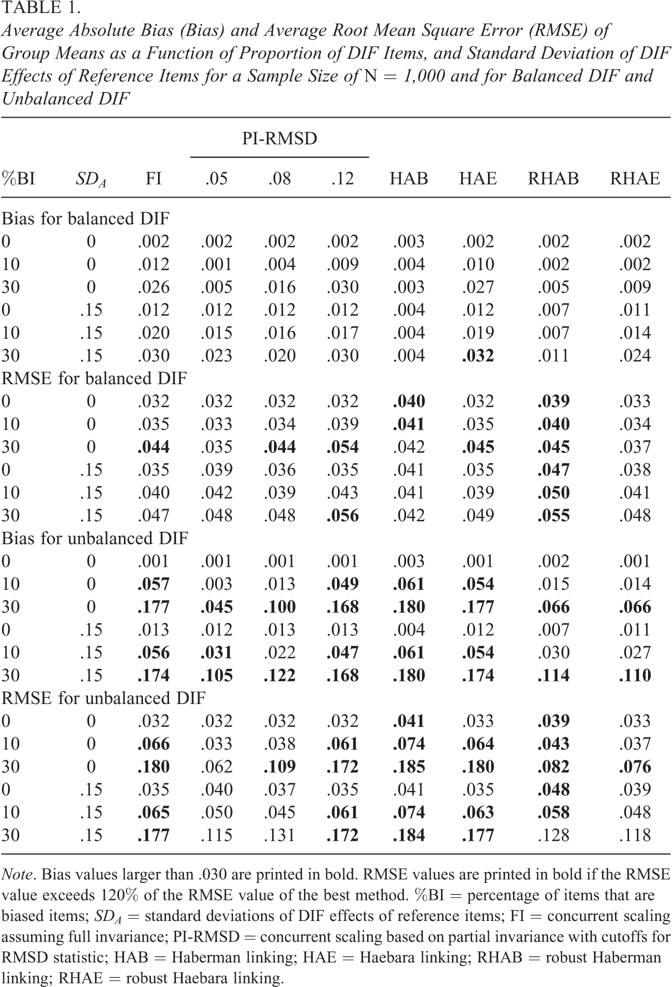
Note. Bias values larger than .030 are printed in bold. RMSE values are printed in bold if the RMSE value exceeds 120% of the RMSE value of the best method. %BI = percentage of items that are biased items; SD_A = standard deviations of DIF effects of reference items; FI = concurrent scaling assuming full invariance; PI-RMSD = concurrent scaling based on partial invariance with cutoffs for RMSD statistic; HAB = Haberman linking; HAE = Haebara linking; RHAB = robust Haberman linking; RHAE = robust Haebara linking.

Table 1 shows the average absolute bias and average RMSE for the conditions with a sample size of N = 1,000. In the case of balanced DIF, all scaling strategies were approximately unbiased or showed only small biases. As can be seen, the HAB approach was superior to both the FI approach and the HAE approach. This finding was expected because the HAB linking approach estimated group means under the assumption that DIF effects sum to zero (see Appendix B, Equation B2). This condition exactly resembled the data-generating model. In contrast, the FI and HAE approach employed a different weighting of DIF effects that resulted in small biases (particularly for a large proportion of biased items; see Appendix A, Equation A7, and Appendix C, Equation C4). Furthermore, concurrent scaling under partial invariance (PI-RMSD) slightly outperformed the FI and HAE approaches in many conditions. The robust linking approaches (RHAB and RHAE) performed similarly to the partial invariance approach using the RMSD cutoff of .05 or .08. For the average RMSE, the results were similar to the findings for the bias. First, country mean estimates that were produced by separate scaling with HAE were not less stable than estimates provided by concurrent scaling under FI (see also Andersson, 2018, for similar findings). Second, the performance of concurrent scaling under partial invariance depended on the choice of the specific cutoff to be used for the RMSD statistic. In many conditions, cutoff values of .05 and .08 for the RMSD statistic—which result in using a larger number of country-specific item parameters—outperformed the cutoff value of .12 and produced country mean estimates that were close to the FI approach in terms of RMSE.

Table 1 also shows the average absolute bias and average RMSE for the conditions with a sample size of N = 1,000 in the case of unbalanced DIF (i.e., all DIF effects of biased items were either positive with a value of δ or negative with a value of −δ for each country). The country mean estimates produced by the FI and nonrobust linking approaches (HAB and HAE) were grossly biased in some conditions. This bias was substantially reduced with the partial invariance approaches (PI-RMSD) and robust linking approaches (RHAB and RHAE). The robust linking approaches based on separate scaling (RHAB and RHAE) performed similarly. They even outperformed the partial invariance approaches based on concurrent scaling in many conditions if an optimal cutoff value for the RMSD was not chosen. Considering the dependency of the RMSD on the sample size, it is noteworthy that the choice of an optimal cutoff for the RMSD statistic was either .05 or .08, and there were no conditions in which the cutoff of .12 was preferred.

Figure 1 shows the influence of sample size on the performance of the selected scaling strategies in the case of unbalanced DIF. It can be concluded that the general findings for N = 1,000 also hold for N = 250 and N = 500. The concurrent scaling under FI and nonrobust linking (HAE) approaches were also more biased than the partial invariance and robust linking (RHAE) approaches in smaller samples. The PI-RMSD approach with a cutoff of .08 was always superior to the cutoff of .12. Importantly, the approaches based on separate scaling (HAE, RHAE) were only less stable than the concurrent scaling approaches (FI, PI-RMSD) with a small sample size of N = 250. HAB produced substantially more variable estimates than all other approaches for N = 250. Hence, for sample sizes larger than 500, the different performance of scaling strategies for the average RMSE was mainly determined by average absolute bias.

Figure 1.

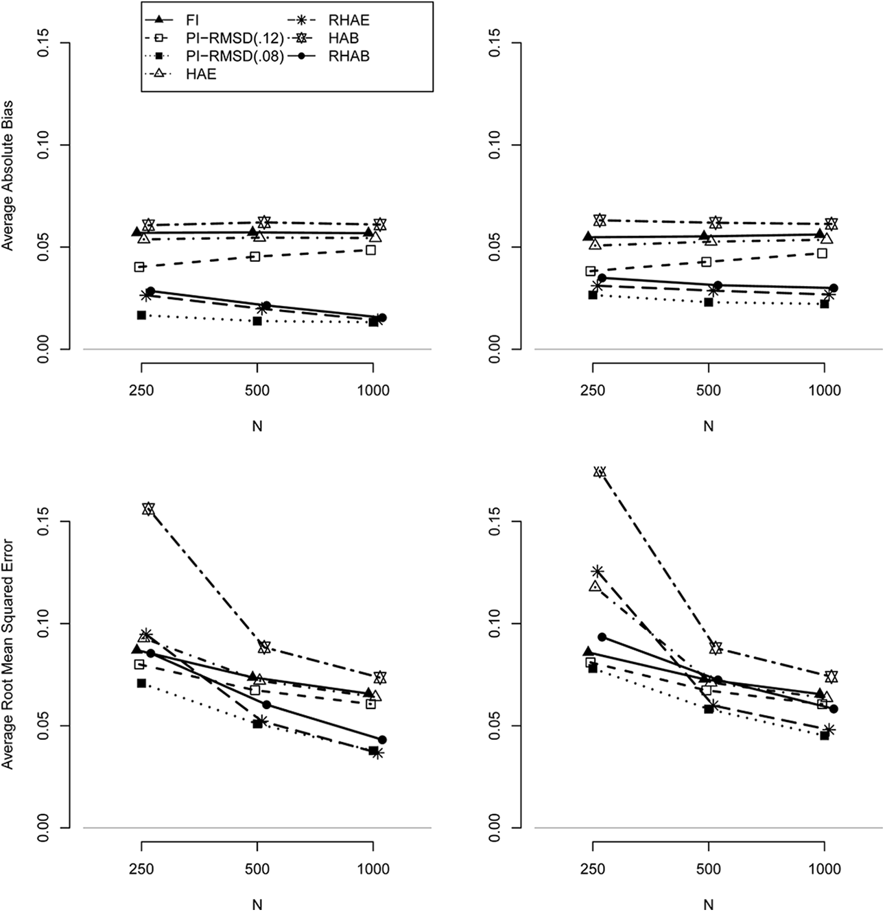
Average absolute bias (upper panels) and average root mean square error (lower panels) for unbalanced differential item functioning (DIF) for 10% biased items with a DIF effect size of .6, I = 20 items, for a standard deviation of DIF effects of reference items of SDA = 0 (left panels) and SDA = 0.15 (right panels) as a function of sample size.

Empirical Example: Cross-Sectional Country Comparisons for Reading in PISA 2006

In order to illustrate the different approaches to estimating country means, we analyzed the data from the PISA 2006 assessment (OECD, 2009). In this reanalysis, we included 26 OECD countries that participated in 2006, and we focused on the reading domain, which was a minor domain in PISA 2006. Thus, reading items were only administered to a subset of the participating students, and we included only those students who received a test booklet with at least one reading item. This resulted in a total sample size of 110,236 students (ranging from 2,010 to 12,142 between countries). In total, 28 reading items nested within eight testlets were used in PISA 2006. Six of the 28 items were polytomous and were dichotomously recoded, with only the highest category being recoded as correct. We used six different methods to obtain estimates of country means: a full invariance approach (concurrent scaling with multiple groups; FI); a partial invariance approach with DIF detection based on the RMSD statistic (PI-RMSD) using the cutoffs .05, .08, and the value of .12 that is used in PISA; two nonrobust linking methods (Haberman, HAB; Haebara HAE), and two robust linking methods (RHAB; RHAE). For all analyses, student weights within a country were normalized to a sum of 5,000 so that all countries contributed equally to the analyses. Finally, all estimated country means were linearly transformed so that the distribution containing all (weighted) students in all 26 countries had a mean of 500 (points) and a standard deviation of 100. Note that this transformation is not equivalent to the one used in officially published PISA publications. The 80 balanced repeated replicate weights defined in PISA were used for computing standard errors (OECD, 2009).

In a first exploratory analysis, we fitted the FI model and computed the RMSD statistic for all items and all countries. The average RMSD across items and countries was .060 (SD = .044). For each item, we also computed the average RMSD across countries. These 28 values ranged between .027 and .099 (SD = .020), where the largest value was obtained for item R227Q02T. The average RMSD at the level of countries ranged between .044 and .082 (SD = .010), where the largest values were obtained for Japan (.082) and South Korea (.080). We also specified a variance component model for the RMSD values using items and countries as random effects. We found that the item factor (16.8% of the total variance) was more important than the country factor (2.6%), but the residual effects had the largest variance contribution (80.5%). When using an RMSD cutoff of .12, 9.8% of the item difficulty parameters received country-specific parameters (cutoff of .08: 23.8%; cutoff of .05: 49.1%).

In a second exploratory analysis, we specified the partial invariance approach using RMSD cutoff values from .02 to .20 in increments of .01. We assessed model fit using the information criteria AIC and BIC as well as the log-penalty measure (see van Rijn et al., 2016). In Table 2, these model fit statistics are displayed for the PI-RMSD models with different RMSD cutoff values. The PI-RMSD model with a cutoff of .02 was preferred by the AIC, and the model with a cutoff of .05 was preferred by the BIC. By using differences in log-penalty measures (i.e., ΔPE in Table 2), the difference between the FI model and the PI-RMSD model with a cutoff of .12 was .0071, which could be considered a small difference according to van Rijn et al. (2016, p. 5). The model with a cutoff value of .08 showed a moderate difference of .0103 to the FI model. Overall, the partial invariance approach resulted in a better model fit than the FI model. However, different fit measures prefer different cutoff values for the RMSD statistic.

Table 2.

Model Comparison of 2PL Model under Full Invariance and Partial Invariance With Different Cutoff Values for the RMSD Statistic

Cutoff	#par	unique	Dev	AIC	BIC	PE	ΔPE
.02	743	88.5	905,279	906,765	913,426	.5016	.0130
.03	629	72.2	905,595	906,853	912,492	.5017	.0129
.04	532	58.8	906,155	907,219	911,988	.5019	.0127
.05	462	49.2	906,888	907,812	911,954	.5022	.0124
.06	391	39.4	907,901	908,683	912,188	.5027	.0119
.07	317	29.1	909,798	910,432	913,273	.5037	.0109
.08	278	23.8	911,041	911,597	914,089	.5043	.0103
.09	241	18.6	912,688	913,170	915,330	.5052	.0094
.10	213	14.8	914,070	914,496	916,406	.5059	.0087
.11	188	11.3	915,809	916,185	917,870	.5068	.0078
.12	172	9.1	917,075	917,419	918,961	.5075	.0071
.13	163	7.9	917,922	918,248	919,709	.5080	.0066
.14	151	6.2	919,289	919,591	920,945	.5087	.0059
.15	145	5.4	920,112	920,402	921,701	.5092	.0054
.16	136	4.1	921,659	921,931	923,151	.5100	.0046
.17	127	2.9	923,472	923,726	924,864	.5110	.0036
.18	123	2.3	924,335	924,581	925,684	.5115	.0031
.19	119	1.8	925,231	925,469	926,536	.5120	.0026
.20	117	1.5	925,795	926,029	927,078	.5123	.0023
FI	106	0	929,995	930,207	931,157	.5146	—

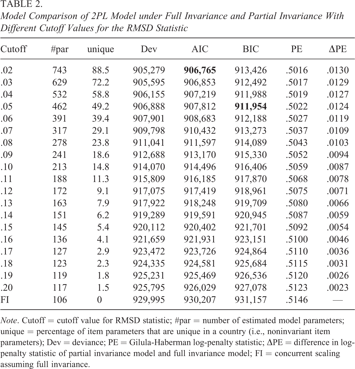
Note. Cutoff = cutoff value for RMSD statistic; #par = number of estimated model parameters; unique = percentage of item parameters that are unique in a country (i.e., noninvariant item parameters); Dev = deviance; PE = Gilula-Haberman log-penalty statistic; ΔPE = difference in log-penalty statistic of partial invariance model and full invariance model; FI = concurrent scaling assuming full invariance.

Table 3.

Country Means for the Reading Domain for PISA 2006 for 26 Selected Organization for Economic Cooperation and Development Countries

Country	N	RMSD			Rg	FI	PI-RMSD			HAB	HAE	RHAB	RHAE
Country	N	M	SD	flag	Rg	FI	.12	.08	.05	HAB	HAE	RHAB	RHAE
AUS	7,562	.052	.034	1	8	517	518	517	523	520	515	521	523
AUT	2,646	.047	.027	1	4	496	497	497	495	499	496	496	495
BEL	4,840	.044	.025	0	6	506	505	506	508	504	506	502	508
CAN	12,142	.051	.036	1	10	528	531	531	527	524	526	521	528
CHE	6,578	.053	.036	1	7	502	504	506	502	499	502	504	503
CZE	3,246	.059	.037	2	5	483	483	483	483	486	483	488	484
DEU	2,701	.055	.040	2	21	496	499	500	498	481	497	502	502
DNK	2,431	.065	.063	4	9	500	501	505	501	505	499	508	503
ESP	10,506	.070	.052	3	10	465	471	466	467	464	466	474	467
EST	2,630	.064	.043	3	9	499	506	502	503	499	497	503	501
FIN	2,536	.048	.044	2	10	552	556	556	550	546	548	549	548
FRA	2,524	.055	.037	1	7	499	502	497	500	498	499	504	500
GBR	7,061	.065	.043	4	7	499	492	496	495	498	497	495	496
GRC	2,606	.069	.072	5	19	457	452	449	452	468	458	457	451
HUN	2,399	.052	.032	1	5	485	485	490	485	485	487	489	489
IRL	2,468	.052	.027	0	6	518	518	518	518	521	517	515	516
ISL	2,010	.056	.036	2	6	493	498	497	496	492	492	495	494
ITA	11,629	.060	.034	2	6	471	472	475	471	474	472	477	473
JPN	3,203	.082	.062	5	19	503	499	494	496	513	507	499	499
KOR	2,790	.080	.061	4	22	556	542	543	553	564	561	543	546
LUX	2,443	.050	.026	0	14	482	482	483	487	473	481	483	486
NLD	2,666	.076	.047	6	14	509	508	508	505	507	511	497	503
NOR	2,504	.071	.052	6	5	489	485	484	487	485	489	489	487
POL	2,968	.062	.038	3	5	507	509	507	509	512	507	509	511
PRT	2,773	.072	.058	6	5	476	476	476	475	480	476	476	475
SWE	2,374	.052	.036	1	13	511	507	513	514	501	509	504	511

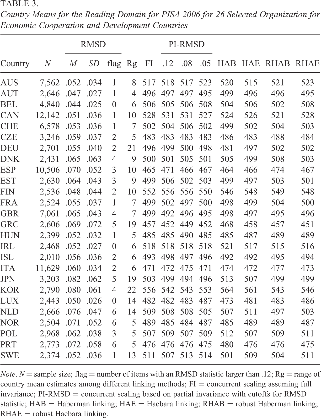
Note. N = sample size; flag = number of items with an RMSD statistic larger than .12; Rg = range of country mean estimates among different linking methods; FI = concurrent scaling assuming full invariance; PI-RMSD = concurrent scaling based on partial invariance with cutoffs for RMSD statistic; HAB = Haberman linking; HAE = Haebara linking; RHAB = robust Haberman linking; RHAE = robust Haebara linking.

In Table 3, the country mean estimates obtained from the six different methods are shown. Within a country, the range of the country’s mean differed between 4 and 22 points (M = 9.7, SD = 5.4) across the different methods. These differences between the methods can be attributed to different amounts of country DIF. It is instructive to first focus on the comparison of country means based on the assumption of full invariance in a concurrent scaling approach that ignores DIF (similar to the PISA method used until 2012) and the partial invariance approach based on the RMSD statistic with a cutoff of .12 (which is the PISA method that has been used since 2015). About 9.8% of all items across countries exceeded an absolute value of .12 for the RMSD statistic. There was an average absolute difference of 3.0 points between the two approaches, with a maximum discrepancy of 22 points (South Korea, KOR). As shown in Table 3, South Korea had four flagged DIF items with an RMSD statistic larger than .12. Those four items received country-specific item parameters in the partial invariance approach, which induced a drop of 14 points in the partial invariance approach (542 points) compared to the full invariance approach (556 points). For all other countries, the absolute differences between the two approaches were at most 7 points (Min = 0, M = 3.0, SD = 3.2). The magnitude of the difference between the full and partial invariance approach with an RMSD cutoff of .12 was, therefore, similar to that of the standard errors caused by person sampling (about 3 points). Hence, the choice of a particular linking method is of practical relevance for at least some countries (but see Jerrim et al., 2018, for a similar analysis with the PISA 2015 data).

Table 4 shows the average absolute differences and correlations of the country mean estimates for the different methods. It needs to be emphasized that even a correlation of country means as high as .996 (FI with HAE) can result in a nonnegligible average absolute difference of 1.3 points (with a maximum of 5 points for South Korea, KOR). The partial invariance approaches based on the RMSD statistic with cutoffs of .08 and .05 performed similarly to the robust Haebara approach (r = .987, .990, .995, respectively). When interpreting the results, it needs to be noted that the observed discrepancies in country means for PISA 2006 could be smaller for more recent PISA assessments as the number of items in a domain has been substantially increased in the recent PISA assessments.

Table 4.

Average Absolute Differences (Upper Diagonal) and Correlations (Lower Diagonal) for Different Linking Methods for Reading Domain in PISA 2006 for 26 Selected Organization for Economic Cooperation and Development Countries

	1	2	3	4	5	6	7	8
1: FI		3.0	3.2	2.3	4.5	1.3	4.4	3.0
2: PI-RMSD .12	.981		2.1	2.7	6.2	3.8	3.5	3.0
3: PI-RMSD .08	.980	.992		2.9	6.4	4.0	4.0	2.7
4: PI-RMSD .05	.991	.986	.987		5.8	3.2	3.9	1.7
5: HAB	.966	.930	.919	.942		4.2	6.2	5.8
6: HAE	.996	.969	.967	.982	.972		4.6	3.4
7: RHAB	.974	.983	.979	.982	.934	.964		3.0
8: RHAE	.986	.988	.990	.995	.933	.977	.987

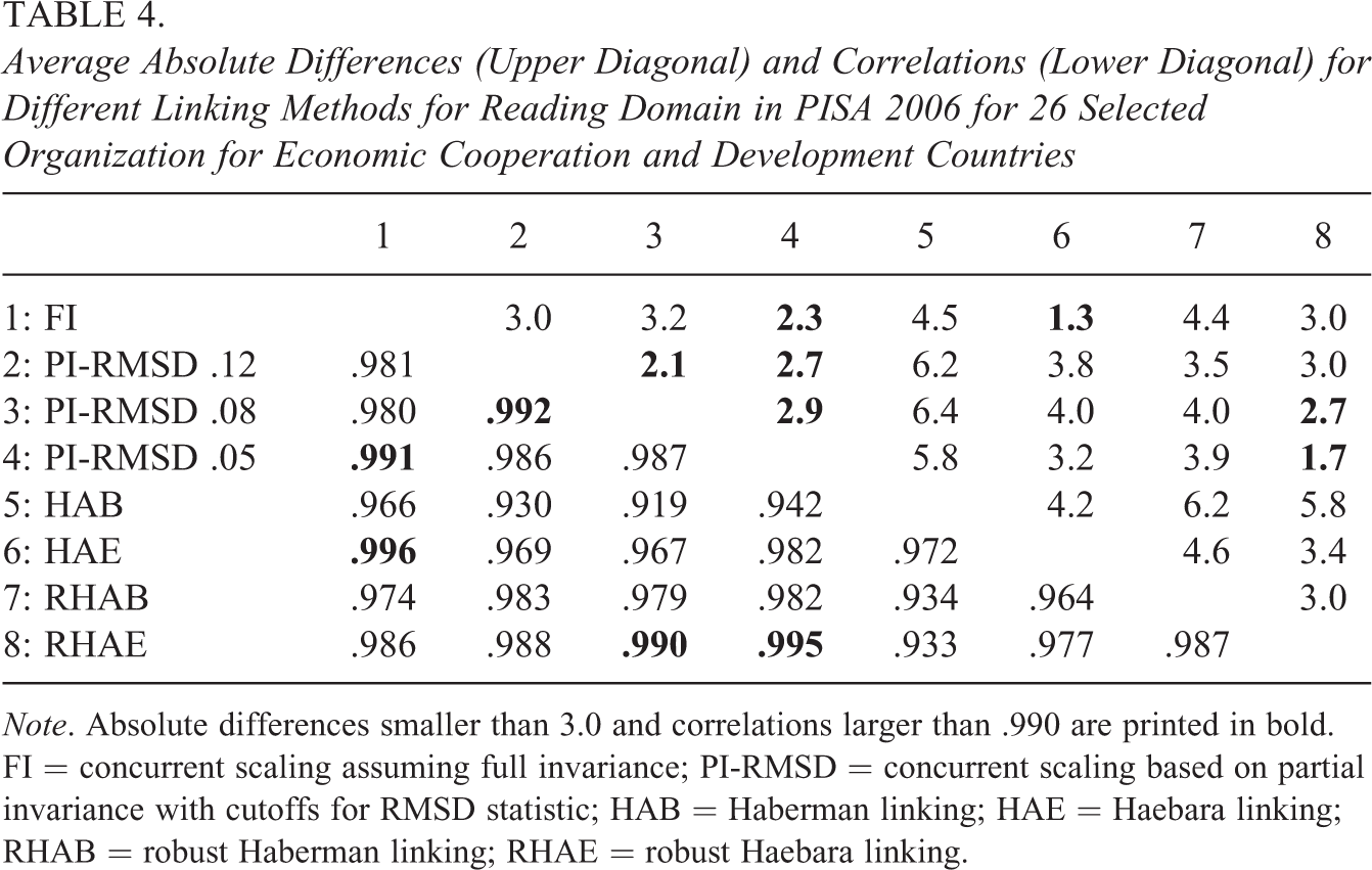
Note. Absolute differences smaller than 3.0 and correlations larger than .990 are printed in bold. FI = concurrent scaling assuming full invariance; PI-RMSD = concurrent scaling based on partial invariance with cutoffs for RMSD statistic; HAB = Haberman linking; HAE = Haebara linking; RHAB = robust Haberman linking; RHAE = robust Haebara linking.

In Table 5, the standard errors for the country means, and the differences between the scaling models and their associated standard errors are displayed. Notably, the country-specific standard errors for the model differences were smaller than the standard errors for the country means because the country means of the different models were strongly dependent as they were obtained from the same data set. For example, the average standard error for the country means under FI was 3.0, while the standard error for the FI and RHAE model difference was 1.9. Notably, 10 out of 26 comparisons between the FI and PI-RMSD(.12) (i.e., the column “FI − PI-RMSD(.12)” in Table 5) turned out to be statistically significant. The difference between the FI (PI-RMSD(.12)) and RHAE models was significant in 6 (or 4, respectively) out of 26 comparisons. To conclude, some model differences are of practical importance.

Table 5.

Standard Errors for Country Means and Differences Between Models for the Reading Domain in PISA 2006 for 26 Selected Organization for Economic Cooperation and Development Countries

	FI		PI-RMSD(.12)		RHAE		FI − PI-RMSD(.12)		FI − RHAE		PI-RMSD(.12) − RHAE
Country	M	SE	M	SE	M	SE	Δ	SE	Δ	SE	Δ	SE
AUS	516.6	2.4	518.0	2.4	523.2	2.9	−1.4	0.5	−6.5	1.4	−5.2	1.6
AUT	496.3	3.7	497.2	3.9	494.8	4.4	−0.9	1.1	1.5	1.8	2.4	2.1
BEL	506.0	3.1	505.3	3.6	508.0	3.3	0.6	2.2	−2.0	1.5	−2.7	2.6
CAN	527.6	2.1	531.0	2.2	528.0	2.5	−3.4	0.5	−0.4	1.5	3.1	1.6
CHE	502.3	3.0	503.8	2.9	503.4	3.3	−1.5	0.5	−1.1	1.6	0.4	1.4
CZE	483.2	4.4	482.9	5.0	483.7	4.5	0.2	2.0	−0.6	2.1	−0.8	3.2
DEU	496.2	4.9	499.0	5.1	502.4	5.2	−2.9	1.8	−6.3	1.8	−3.4	2.5
DNK	500.1	3.1	500.9	4.4	503.3	3.3	−0.8	3.3	−3.2	1.6	−2.4	3.9
ESP	464.8	2.2	471.1	2.6	467.0	2.4	−6.3	1.5	−2.2	1.3	4.1	1.8
EST	499.3	2.9	506.2	2.9	501.1	3.1	−6.8	0.6	−1.8	2.2	5.0	2.1
FIN	551.6	2.4	556.3	2.5	547.6	3.0	−4.6	0.5	4.0	2.0	8.7	1.9
FRA	499.1	3.8	502.2	4.2	500.1	4.2	−3.1	1.1	−1.0	2.3	2.1	2.4
GBR	498.5	2.4	492.5	2.4	496.2	3.0	6.0	1.1	2.4	1.6	−3.7	2.0
GRC	456.9	3.4	452.3	4.4	451.0	3.7	4.6	2.9	5.9	1.4	1.3	3.3
HUN	485.2	3.3	485.4	4.4	488.8	4.1	−0.2	2.3	−3.6	2.3	−3.4	2.9
IRL	518.4	3.4	517.8	3.3	515.7	4.5	0.6	0.4	2.7	2.3	2.1	2.5
ISL	493.2	1.9	497.7	3.0	493.7	2.8	−4.5	2.3	−0.6	1.9	3.9	3.0
ITA	471.4	2.2	472.0	2.1	472.5	3.0	−0.5	0.6	−1.1	1.9	−0.6	1.9
JPN	503.0	3.5	498.9	4.8	499.1	4.9	4.1	3.1	3.9	2.8	−0.2	3.8
KOR	556.2	3.7	542.0	3.6	546.5	4.2	14.2	0.7	9.7	2.4	−4.5	2.4
LUX	482.0	2.2	481.7	3.4	486.5	2.7	0.3	2.7	−4.5	1.8	−4.8	2.5
NLD	509.4	3.0	507.8	4.6	503.1	4.5	1.6	3.4	6.3	3.0	4.7	5.0
NOR	489.4	2.7	485.4	2.6	487.1	3.2	3.9	1.2	2.2	2.2	−1.7	2.5
POL	506.8	2.6	509.4	3.0	510.7	3.3	−2.6	2.0	−3.9	2.1	−1.2	2.7
PRT	475.8	3.3	475.8	3.5	475.0	3.7	0.1	1.1	0.8	1.7	0.8	1.8
SWE	510.7	2.9	507.3	4.4	511.5	3.4	3.4	2.8	−0.8	1.7	−4.2	3.2
Aver. Abs.	500	3.0	500	3.5	500	3.6	3.1	1.6	3.0	1.9	3.0	2.6

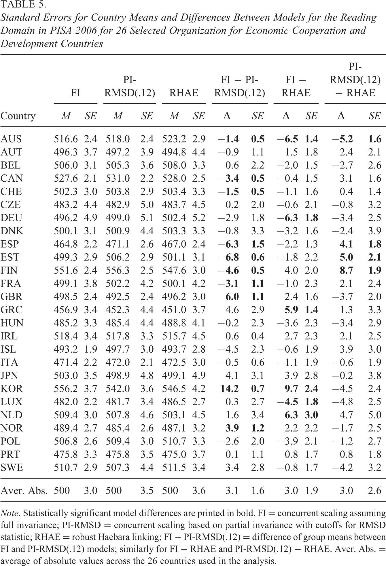
Note. Statistically significant model differences are printed in bold. FI = concurrent scaling assuming full invariance; PI-RMSD = concurrent scaling based on partial invariance with cutoffs for RMSD statistic; RHAE = robust Haebara linking; FI − PI-RMSD(.12) = difference of group means between FI and PI-RMSD(.12) models; similarly for FI − RHAE and PI-RMSD(.12) − RHAE. Aver. Abs. = average of absolute values across the 26 countries used in the analysis.

Discussion

In this article, we discussed concurrent and separate scaling approaches for comparing group means in the presence of DIF effects. We analytically showed that concurrent scaling under full invariance, concurrent scaling under partial invariance, and separate scaling with linking place different constraints on the DIF effects of reference items and biased items. In a simulation study, we showed that the performance of the different approaches depended on the nature of the DIF effects, particularly for the biased items (balanced vs. unbalanced DIF). In the case of unbalanced DIF, we found that concurrent scaling under full invariance and separate scaling with nonrobust linking produced biased country mean estimates. In contrast, concurrent scaling under partial invariance and separate scaling with robust linking could considerably reduce the bias by removing the impact of items with large DIF effects from the country comparisons. However, the performance of the partial invariance approach strongly depended on the specification of an adequate cutoff value for the RMSD statistic. In most conditions, a cutoff value of .05 performed better than a value of .12. Importantly, with a less than optimal cutoff value for the RMSD statistic, concurrent scaling under partial invariance was outperformed by separate scaling with subsequent robust linking (RHAB, RHAE).

As is the case for all simulation studies, conclusions are limited to the conditions that were investigated in our study. First, we did not consider the case of nonuniform DIF (i.e., DIF that is also present in item slopes) in the data-generating model. It is an interesting topic for future research to examine whether our findings can be generalized to this case. Although one could use similar cutoff values for the RMSD statistics, the linking approaches need further consideration by including item slope parameters. However, it should be noted that uniform DIF is more frequently found in ILSA than nonuniform DIF (Rutkowski & Svetina, 2017). Second, we restricted ourselves to a simulation study involving only 20 items. A linking study for the Rasch model found practically no differences for 20 and 40 items (Robitzsch & Lüdtke, 2020). Further studies could investigate larger numbers of items or could treat items as random instead of as fixed. Third, we assumed that the maximum proportion of biased items was 30%. We believe that the test construction would not have been successful if the majority of items were biased items (Magis & De Boeck, 2011). Third, we only chose two extreme DIF conditions for biased items, namely, the case of balanced DIF in which the DIF effects of biased items sum to zero and the case of unbalanced DIF in which all items either have a joint positive or negative biasing DIF effect δ. In reality, DIF effects of biased items are likely to follow a distribution between these two extreme scenarios. These constellations should be investigated in future simulation studies, providing more practical guidelines for choosing between different scaling approaches.

Our treatment of concurrent and separate scaling approaches for comparing group means in the presence of DIF can be extended in several ways. First, the linking methods could be investigated for polytomous data or the 3PL model, and, again, we would not expect very different findings compared to the 2PL model. However, again, the choice of a cutoff value for the RMSD item fit statistic is crucial for concurrent calibration under partial invariance (Buchholz & Hartig, 2019). Second, different linking functions could be considered. Besides the absolute value loss function $ρ (x) = |x|$ used in robust linking, the loss functions $ρ (x) = {|x|}^{0.25}$ and $ρ (x) = {|x|}^{0.5}$ are used in the invariance alignment approach (DeMars, 2020; Muthén & Asparouhov, 2014). Third, country comparisons for scales in questionnaire data in ILSA are an important outcome (Buchholz & Hartig, 2019; Rutkowski & Svetina, 2017). In this case, linking polytomous item responses based on a low number of items (e.g., I = 5) is of particular interest.

In large-scale assessment studies, the ability distributions are typically estimated using plausible values (von Davier & Sinharay, 2014). Covariates (i.e., background variables) are used in a latent regression model to compute plausible values. Notably, we did not use covariates in our study. However, we expect that our results would also hold if a latent regression model is used. The critical factor is whether the distribution of the ability in a group is correctly specified. In our simulation, we used a normal distribution in each group, and the effect on possible biased estimates would be more significant in short tests. Possible distributional misspecifications in a latent regression model refer only to the regression residuals of the ability variable, so it can be expected that distributional violations are more critical without covariates than with covariates. In future research, the influence of more complex ability distributions (i.e., asymmetric or mixture distributions) on estimated group means could be investigated under a misspecified ability distribution (i.e., assuming a normal distribution).

The linking of multiple groups in the presence of DIF can alternatively be carried out using regularization techniques. In a regularization-based approach to DIF, group-specific item parameters are decomposed into common item parameters and group-specific deviations (e.g., Liang & Jacobucci, 2020; Schauberger & Mair, 2020). Using conventional maximum likelihood estimation would result in a nonidentified model. In the regularization approach, penalty terms for the nonidentifiable group-specific deviations are subtracted from the log-likelihood function to define the optimization function, ensuring the empirical identifiability of model parameters and imposes assumptions about the distribution of the parameters of noninvariance. For example, the lasso penalty function is particularly suited to partial invariance situations (Liang & Jacobucci, 2020).

Furthermore, we believe that conducting a separate estimation with subsequent linking has several advantages over concurrent scaling that relies on full or partial invariance (see Andersson, 2018). Computation times are usually substantially lower with separate estimation. In our empirical example involving 26 countries and 28 items, separate scaling only took about 1 min, and the subsequent Haberman and Haebara linking approaches took at most 3 s, while concurrent scaling assuming full or partial invariance needed 5–10 min by using a multiple-group IRT model. It is often easier to diagnose potential estimation problems with separate estimation (Andersson, 2018). Finally, concurrent scaling can only provide more efficient estimates than separate scaling if model assumptions hold (Kolen & Brennan, 2014). As it cannot be ensured that there are no unmodeled DIF effects or that strict unidimensionality holds, situations in which concurrent scaling should be preferred are not very likely to occur (cf. von Davier et al., 2019, for an alternative view).

In the literature, it is often argued that at least partial invariance for item intercepts is needed to allow meaningful comparisons of group means (e.g., van de Vijver, 2019; Vandenberg & Lance, 2000). However, one critical aspect of the partial invariance approach (as well as other approaches that result in the removal or downweighting of the contribution of particular items, such as robust Haberman or robust Haebara linking) is that comparisons of different groups rely on different sets of items. We regard this feature as a potential threat to validity and find this practice problematic because it compares apples with oranges (see also El-Masri & Andrich, 2020). For example, the comparison of the country means for Germany with those for Italy in PISA does not involve a full set of common item parameters for each country if the sets of country-specific noninvariant items—that receive country-specific item parameters—differ between the two countries. More critically, in the current operational use since PISA 2015, the determination of how a country comparison is conducted (i.e., which items are used as reference items) is solely based on the item misfit in a psychometric model (von Davier et al., 2019). In contrast, approaches using full invariance or complete noninvariance rely on the same set of items for country comparisons. Until PISA 2015, items with DIF effects were only declared as DIF items if translation issues were confirmed (Adams, 2003). In this procedure, items with substantial DIF effects—but without translation issues—remained in a country comparison and were neither removed from scaling nor received country-specific parameters. To conclude, it has to be acknowledged that, in the presence of DIF, country comparisons depend on the particular identification constraint chosen, however arbitrary that choice may be.

Footnotes

Appendix

Notes

References

Adams

R. J.

(2003). Response to “Cautions on OECD’s recent educational survey (PISA).” Oxford Review of Education, 29(3), 379–389. https://doi.org/10.1080/03054980307445

Andersson

(2018). Asymptotic variance of linking coefficient estimators for polytomous IRT models. Applied Psychological Measurement, 42(3), 192–205. https://doi.org/10.1177/0146621617721249

Arai

Mayekawa

S. I.

(2011). A comparison of equating methods and linking designs for developing an item pool under item response theory. Behaviormetrika, 38(1), 1–16. https://doi.org/10.2333/bhmk.38.1

Battauz

(2015). Factors affecting the variability of IRT equating coefficients. Statistica Neerlandica, 69, 85–101. https://doi.org/10.1111/stan.12048

Battauz

(2017). Multiple equating of separate IRT calibrations. Psychometrika, 82(3), 610–636. https://doi.org/10.1007/s11336-016-9517-x

Battauz

(2019). On Wald tests for differential item functioning detection. Statistical Methods & Applications, 28, 103–118. https://doi.org/10.1007/s10260-018-00442-w

Bechger

T. M.

Maris

(2015). A statistical test for differential item pair functioning. Psychometrika, 80(2), 317–340. https://doi.org/10.1007/s11336-014-9408-y

Birnbaum

(1968). Some latent trait models and their use in inferring an examinee’s ability. In Lord

F. M.

Novick

M. R.

(Eds.), Statistical theories of mental test scores (pp. 397–479). MIT Press.

Buchholz

Hartig

(2019). Comparing attitudes across groups: An IRT-based item-fit statistic for the analysis of measurement invariance. Applied Psychological Measurement, 43(3), 241–250. https://doi.org/10.1177/0146621617748323

10.

Burnham

D. R.

Anderson

K. P.

(2002). Model selection and multimodel inference: A practical information-theoretic approach. Springer. https://doi.org/10.1007/b97636

11.

Byrne

B. M.

Shavelson

R. J.

Muthén

(1989). Testing for the equivalence of factor covariance and mean structures: The issue of partial measurement invariance. Psychological Bulletin, 105, 456–466. https://doi.org/10.1037/0033-2909.105.3.456

12.

Byrne

B. M.

van de Vijver

F. J. R.

(2017). The maximum likelihood alignment approach to testing for approximate measurement invariance: A paradigmatic cross-cultural application. Psicothema, 29(4), 539–551. https://doi.org/10.7334/psicothema2017.178

13.

Camilli

(1993). The case against item bias detection techniques based on internal criteria: Do item bias procedures obscure test fairness issues? In Holland

P. W.

Wainer

(Eds.), Differential item functioning: Theory and practice (pp. 397–417). Erlbaum.

14.

DeMars

C. E.

(2020). Alignment as an alternative to anchor purification in DIF analyses. Structural Equation Modeling, 27(1), 56–72. https://doi.org/10.1080/10705511.2019.1617151

15.

El Masri

Y. H.

Andrich

(2020). The trade-off between model fit, invariance, and validity: The case of PISA science assessments. Applied Measurement in Education, 33(2), 174–188. https://doi.org/10.1080/08957347.2020.1732384

16.

Fox

(2016). Applied regression analysis and generalized linear models. Sage.

17.

Fox

J.-P.

Koops

Feskens

Beinhauer

(2020). Bayesian covariance structure modelling for measurement invariance testing. Behaviormetrika, 47(2), 385–410. https://doi.org/10.1007/s41237-020-00119-3

18.

Fox

J.-P.

Mulder

Sinharay

(2017). Bayes factor covariance testing in item response models. Psychometrika, 82(4), 979–1006. https://doi.org/10.1007/s11336-017-9577-6

19.

Fox

J.-P.

Verhagen

A. J.

(2010). Random item effects modeling for cross-national survey data. In Davidov

Schmidt

Billiet

(Eds.), Cross-cultural analysis: Methods and applications (pp. 461–482). Routledge Academic.

20.

Gomez-Benito

Sireci

Padilla

J. L.

Hidalgo

M. D.

Benitez

(2018). Differential item functioning: Beyond validity evidence based on internal structure. Psicothema, 30(1), 104–109. https://doi.org/10.7334/psicothema2017.183

21.

Haberman

S. J.

(2009). Linking parameter estimates derived from an item response model through separate scalings (Research Report RR-09-40). Educational Testing Service. https://doi.org/10.1002/j.2333-8504.2009.tb02197.x

22.

Haberman

S. J.

Lee

Y.-H.

Qian

(2009). Jackknifing techniques for evaluation of equating accuracy (Research Report RR-09-02). Educational Testing Service. https://doi.org/10.1002/j.2333-8504.2009.tb02196.x

23.

Haebara

(1980). Equating logistic ability scales by a weighted least squares method. Japanese Psychological Research, 22(3), 144–149. https://doi.org/10.4992/psycholres1954.22.144

24.

Cui

(2020). Evaluating robust scale transformation methods with multiple outlying common items under IRT true score equating. Applied Psychological Measurement, 44(4), 296–310. https://doi.org/10.1177/0146621619886050

25.

Cui

Fang

Chen

(2013). Using a linear regression method to detect outliers in IRT common item equating. Applied Psychological Measurement, 37(7), 522–540. https://doi.org/10.1177/0146621613483207

26.

Cui

Osterlind

S. J.

(2015). New robust scale transformation methods in the presence of outlying common items. Applied Psychological Measurement, 39(8), 613–626. https://doi.org/10.1177/0146621615587003

27.

Holland

P. W.

Wainer

(Eds.). (1993). Differential item functioning: Theory and practice. Erlbaum.

28.

Jerrim

Parker

Choi

Chmielewski

A. K.

Sälzer

Shure

(2018). How robust are cross-country comparisons of PISA scores to the scaling model used? Educational Measurement: Issues and Practice, 37(4), 28–39. https://doi.org/10.1111/emip.12211

29.

Kankaraš

Moors

(2014). Analysis of cross-cultural comparability of PISA 2009 scores. Journal of Cross-Cultural Psychology, 45(3), 381–399. https://doi.org/10.1177/0022022113511297

30.

Koenker

(2017). Quantile regression: 40 years on. Annual Review of Economics, 9, 155–176. https://doi.org/10.1146/annurev-economics-063016-103651

31.

Köhler

Robitzsch

Hartig

(2020). A bias corrected RMSD item fit statistic: An evaluation and comparison to alternatives. Journal of Educational and Behavioral Statistics, 45(3), 251–273. https://doi.org/10.3102/1076998619890566

32.

Kolen

M. J.

Brennan

R. L.

(2014). Test equating, scaling, and linking. Springer. https://doi.org/10.1007/978-1-4939-0317-7

33.

Kolenikov

(2010). Resampling variance estimation for complex survey data. The Stata Journal, 10(2), 165–199. https://doi.org/10.1177/1536867X1001000201

34.

Kolenikov

(2011). Biases of parameter estimates in misspecified structural equation models. Sociological Methodology, 41(1), 119–157. https://doi.org/10.1111/j.1467-9531.2011.01236.x

35.

Kopf

Zeileis

Strobl

(2015). Anchor selection strategies for DIF analysis: Review, assessment, and new approaches. Educational and Psychological Measurement, 75(1), 22–56. https://doi.org/10.1177/0013164414529792

36.

Kuha

Moustaki

(2015). Nonequivalence of measurement in latent variable modeling of multigroup data: A sensitivity analysis. Psychological Methods, 20(4), 523–536. https://doi.org/10.1037/met0000031

37.

Lang

(1974). A first course in calculus. Addison-Wesley.

38.

Liang

Jacobucci

(2020). Regularized structural equation modeling to detect measurement bias: Evaluation of lasso, adaptive lasso, and elastic net. Structural Equation Modeling, 27(5), 722–734. https://doi.org/10.1080/10705511.2019.1693273

39.

Macaskill

(2008). Alternative scaling models and dependencies in PISA. TAG(0809)6a, TAG Meeting Sydney, Australia. https://bit.ly/35WwBPg

40.

Magis

Beland

Tuerlinckx

De Boeck

(2010). A general framework and an R package for the detection of dichotomous differential item functioning. Behavior Research Methods, 42, 847–862. https://doi.org/10.3758/BRM.42.3.847

41.

Magis

De Boeck

(2011). Identification of differential item functioning in multiple-group settings: A multivariate outlier detection approach. Multivariate Behavioral Research, 46(5), 733–755. https://doi.org/10.1080/00273171.2011.606757

42.

Mellenbergh

G. J.

(1989). Item bias and item response theory. International Journal of Educational Research, 13, 127–143. https://doi.org/10.1016/0883-0355(89)90002-5.

43.

Meredith

(1993). Measurement invariance, factor analysis and factorial invariance. Psychometrika, 58(4), 525–543. https://doi.org/10.1007/BF02294825

44.

Millsap

R. E.

(2011). Statistical approaches to measurement invariance. Routledge. https://doi.org/10.4324/9780203821961

45.

Monseur

Sibberns

Hastedt

(2008). Linking errors in trend estimation for international surveys in education. IERI Monograph Series: Issues and Methodologies in Large-Scale Assessments, 1, 113–122.

46.

Muthén

Asparouhov

(2014). IRT studies of many groups: The alignment method. Frontiers in Psychology, 5, 978. https://doi.org/10.3389/fpsyg.2014.00978

47.

Ogasawara

(2002). Stable response functions with unstable item parameter estimates. Applied Psychological Measurement, 26(3), 239–254. https://doi.org/10.1177/0146621602026003001

48.

Oliveri

M. E.

von Davier

(2011). Investigation of model fit and score scale comparability in international assessments. Psychological Test and Assessment Modeling, 53(3), 315–333.

49.

Organization for Economic Cooperation and Development. (2009). PISA 2006 technical report. OECD Publishing.

50.

Organization for Economic Cooperation and Development. (2015). PISA 2015 field trial analysis report. Outcomes of the cognitive assessment (JT03371930). OECD Publishing.

51.

Organization for Economic Cooperation and Development. (2017). PISA 2015 technical report. OECD Publishing.

52.

Penfield

R. D.

Camilli

(2007). Differential item functioning and item bias. In Rao

C. R.

Sinharay

(Eds.), Handbook of statistics, Vol. 26: Psychometrics (pp. 125–167). Elsevier. https://doi.org/10.1016/S0169-7161(06)26005-X

53.

R Core Team. (2020). R: A language and environment for statistical computing. R Core Team. https://www.R-project.org/

54.

Robitzsch

(2020a). L_p loss functions in invariance alignment and Haberman linking with few or many groups. Stats, 3(3), 246–283. https://doi.org/10.3390/stats3030019

55.

Robitzsch

(2020b). Robust Haebara linking for many groups: Performance in the case of uniform DIF. Psych, 2(3), 155–173. https://doi.org/10.3390/psych2030014

56.

Robitzsch

(2020c). sirt: Supplementary item response theory models (R package version 3.9-4). https://CRAN.R-project.org/package=sirt

57.

Robitzsch

Kiefer

(2020). TAM: Test analysis modules (R package version 3.4-26). http://CRAN.R-project.org/package=TAM

58.

Robitzsch

Lüdtke

(2020). A review of different scaling approaches under full invariance, partial invariance, and noninvariance for cross-sectional country comparisons in large-scale assessments. Psychological Test and Assessment Modeling, 62(2), 233–279.

59.

Rutkowski

Svetina

(2017). Measurement invariance in international surveys: Categorical indicators and fit measure performance. Applied Measurement in Education, 30(1), 39–51. https://doi.org/10.1080/08957347.2016.1243540

60.

Schauberger

Mair

(2020) A regularization approach for the detection of differential item functioning in generalized partial credit models. Behavior Research Methods, 52, 279–294. https://doi.org/10.3758/s13428-019-01224-2

61.

Soares

T. M.

Goncalves

F. B.

Gamerman

(2009). An integrated Bayesian model for DIF analysis. Journal of Educational and Behavioral Statistics, 34(3), 348–377. https://doi.org/10.3102/1076998609332752

62.

Sueiro

M. J.

Abad

F. J.

(2011). Assessing goodness of fit in item response theory with nonparametric models: A comparison of posterior probabilities and kernel-smoothing approaches. Educational and Psychological Measurement, 71(5), 834–848. https://doi.org/10.1177/0013164410393238

63.

Tijmstra

Liaw

Bolsinova

Rutkowski

(2020). Sensitivity of the RMSD for detecting item-level misfit in low-performing countries. Journal of Educational Measurement, 57(4), 566–583. https://doi.org/10.1111/jedm.12263

64.

Vandenberg

R. J.

Lance

C. E.

(2000). A review and synthesis of the measurement invariance literature: Suggestions, practices, and recommendations for organizational research. Organizational Research Methods, 3(1), 4–70. https://doi.org/10.1177/109442810031002

65.

van de Schoot

Kluytmans

Tummers

Lugtig

Hox

Muthén

(2013). Facing off with Scylla and Charybdis: A comparison of scalar, partial, and the novel possibility of approximate measurement invariance. Frontiers in Psychology, 4, 770. https://doi.org/10.3389/fpsyg.2013.00770

66.

van de Vijver

F. J. R.

(2019). Invariance alignment in large-scale studies. OECD. https://doi.org/10.1787/254738dd-en

67.

van Rijn

P. W.

Sinharay

Haberman

S. J.

Johnson

M. S.

(2016). Assessment of fit of item response theory models used in large-scale educational survey assessments. Large-Scale Assessments in Education, 4, 10. https://doi.org/10.1186/s40536-016-0025-3

68.

Verhagen

Levy

Millsap

R. E.

Fox

J. P.

(2016). Evaluating evidence for invariant items: A Bayes factor applied to testing measurement invariance in IRT models. Journal of Mathematical Psychology, 72, 171–182. https://doi.org/10.1016/j.jmp.2015.06.005

69.

von Davier

Sinharay

(2014). Analytics in international large-scale assessments: Item response theory and population models. In Rutkowski

von Davier

Rutkowski

(Eds.), Handbook of international large-scale assessment (pp. 155–174). Boca Raton: CRC Press. https://doi.org/10.1201/b16061

70.

von Davier

Yamamoto

Shin

H. J.

Chen

Khorramdel

Weeks

Davis

Kong

Kandathil

(2019). Evaluating item response theory linking and model fit for data from PISA 2000–2012. Assessment in Education: Principles, Policy & Practice, 26(4), 466–488. https://doi.org/10.1080/0969594X.2019.1586642

71.

White

(1982). Maximum likelihood estimation of misspecified models. Econometrica, 50(1), 1–25. https://doi.org/10.2307/1912526

72.

Yamamoto

Khorramdel

von Davier

(2013). Scaling PIAAC cognitive data. In OECD (Eds.), Technical report of the survey of adult skills (PIAAC) (pp. 408–440). Paris: OECD Publishing. https://bit.ly/32Y1TVt

73.

Zwitser

R. J.

Glaser

S. S. F.

Maris

(2017). Monitoring countries in a changing world: A new look at DIF in international surveys. Psychometrika, 82(1), 210–232. https://doi.org/10.1007/s11336-016-9543-8

Mean Comparisons of Many Groups in the Presence of DIF: An Evaluation of Linking and Concurrent Scaling Approaches

Abstract

Keywords

Uniform DIF in the 2PL Model

Scaling Approaches for Multiple-Group Comparisons

Concurrent Scaling Under Full Invariance

Concurrent Scaling Under Partial Invariance Using DIF Statistics

Linking With Separate Scaling Under Full Noninvariance

Haberman linking

Haebara linking

Computation of Standard Errors

Research Questions

Simulation Study

Simulated Conditions

Analysis Models and Criteria

Results

Empirical Example: Cross-Sectional Country Comparisons for Reading in PISA 2006

Discussion

Footnotes

Appendix

Notes

References