EEG connectivity analysis in infants: A Beginner’s Guide on Preprocessing and Processing Techniques

Abstract

Over the last decades, infantile brain networks have received increased scientific attention due to the elevated need to understand better the maturational processes of the human brain and the early forms of neural abnormalities. Electroencephalography (EEG) is becoming a popular tool for the investigation of functional connectivity (FC) of the immature brain, as it is easily applied in awake, non-sedated infants. However, there are still no universally accepted standards regarding the preprocessing and processing analyses which address the peculiarities of infantile EEG data, resulting in comparability difficulties between different studies. Nevertheless, during the last few years, there is a growing effort in overcoming these issues, with the creation of age-appropriate pipelines. Although FC in infants has been mostly measured via linear metrics and particularly coherence analysis, non-linear methods, such as cross-frequency-coupling (CFC), may be more valuable for the investigation of network communication and early network development. Additionally, graph theory analysis often accompanies linear and non-linear FC computation offering a more comprehensive understanding of the infantile network architecture. The current review attempts to gather the basic information on the preprocessing and processing techniques that are usually employed by infantile FC studies, while providing guidelines for future studies.

1 Introduction

The human brain is composed of anatomically different large-scaled networks, such as the default mode network, which are comprised of widespread but functionally connected components [1–3]. FC refers to the temporal relationship (or synchronization) between the activity of different brain regions [4, 5]. Studying the development of neural networks from infancy to adulthood has been a topic of great interest with many researchers investigating their association with cognitive abilities such as learning, memory, attention or intelligence [6–10] and various neurodevelopmental disorders such as autistic spectrum disorder (ASD) [11, 12], attentional deficit and hyperactive disorder (ADHD) [13] and reading difficulties [14, 15].

In general, brain networks can be measured via various methods, during both resting (not participating in any cognitive task) and active state (participating in cognitive tasks such as visual attention or working memory) [16–18]. Traditionally, functional magnetic resonance imaging (fMRI) has been one of the most popular choices for the computation of neural network FC in the adult [19, 20] and infantile brain [21, 22].

Over the last couple decades, EEG has gained more and more popularity for the study of brain as it is a relative inexpensive tool with high temporal resolution [23, 24], rendering it more suitable for FC analysis in contrast with fMRI which provides slower and indirect measurements of neural activity [25]. In fact, EEG is often preferred over fMRI when studying the immature brain as it is easily applied in awake and non-sedated infants, while being able to withstand motor-artifacts at a larger degree [26–28]. Despite its low spatial resolution, many researchers have demonstrated that brain FC measurement via EEG is comparable with that of fMRI [29–32]. Notably, FC analysis with EEG has been successfully performed in infants as early as one day [33].

In EEG, the most common technique to analyze FC is by calculating localized or widespread oscillatory (phase or amplitude) synchrony between different time points or trials [18]. These methods can be either linear or non-linear [34].

Coherence has been for decades one of the most common linear applied metric for FC analysis in adults [35–38] and infants [39–42] with several studies providing insight on network development. Other common linear metrics are cross-correlation, phase slope index (PSI) [43], phase lag index (PLI) [44], phase-locking value (PLV) [45]. On the other hand, CFC and graph theory analysis are two statistical methods that can overcome the practical obstructions of linear FC metrics. In fact, non-linear FC analysis could potentially be more suitable for the study of network communication and network development of the immature brain, which, as previously mentioned, follows both linear and non-linear developmental processes [8, 39, 46]. Nevertheless, CFC and graph analysis have been less employed in infants, with several of aspects of them remaining vague and under debate.

The interpretation of the EEG FC analysis still remains a difficult task, especially in the pediatric population, as there is not a general consensus on the details of data preprocessing and main processing, with adult standards often being applied in infants. Only recently, three infantile preprocessing pipelines were published by Gabard-Durnam et al. [47], Debnath et al. [48] and Fló et al. [49], emphasizing that the infantile EEG recordings often have different characteristics, such as more motor artifacts and shorter length, and suggesting the use of more intricate and flexible procedures. Secondly, the low spatial resolution of the EEG, due to signal diffusion, constitutes the task of cortical source-localization of the electrical signal more challenging [18], with infantile studies requiring specially designed processes that take into consideration the unique brain and EEG infantile characteristics [50, 51].

The present review aims to organize and systematize research on infantile FC through EEG analysis, with a particular focus on those studies that employed coherence analysis (twenty collected articles), CFC analysis (seven collected articles), and graph theory analysis (eight collected articles). Its additional goal is to act as a guide for the investigation of the developing brain networks while providing information on the limitations in preprocessing and processing of the EEG data, and the current efforts from various researchers to overcome these issues. Ultimately, the increase of knowledge regarding the infantile EEG characteristics and the creation of age-appropriate preprocessing and processing standards could lead to less discrepancies between the different studies and eventually into creating an easy-applied tool to measure the immature brain networks of awake and unsedated individuals.

2 Basic Infantile Head and Brain Characteristics

Before the commencement of the study and data collection, the researcher must keep in mind the different characteristics of the infantile head and brain that are relevant to the subsequent EEG data analysis, including FC measurement and the creation of realistic head models.

Initially, some of the prominent head anatomical features of infants that interest the researcher are the elevated skull conductivity, thinner skull thickness, and the presence of soft spots (i.e. fontanels and sutures) [50–53]. These characteristics are associated with higher volume conduction during EEG recording. Secondly, it is important to consider the state of infantile neural networks and their developmental patterns. These patterns exhibit both linear and non-linear trajectories, depending on the maturation stage and brain region [8, 39, 40, 46]. Multiple MRI and fMRI studies have indicated that the structural and functional development of primary neural networks (e.g., visual, auditory, sensorimotor networks) precedes that of higher-order networks (e.g., default mode, salience, dorsal attentional, ventral attentional, fronto-parietal, and limbic networks), with the prefrontal cortex being the last region to be fully functionally integrated [1, 8, 54–56].

Additionally, infantile neural networks are characterized by distinct anatomical features, often occupying different neural components. Specifically, while some theories suggest that immature neural networks initially exhibit widespread, chaotic, and random FC, gradually evolving into ‘small-world’ functional systems [33, 55, 57–61], recent EEG studies employing graph theory analysis have questioned this perspective. Particularly, they have argued that even very young infants demonstrate organized networks, particularly in their frontal and parietal regions [33, 62]. The debate also continues regarding whether the developing brain shifts from short-distance to long-distance neural activity [8, 56, 63, 64] or vice versa [39, 40, 65]. Consequently, measures such as coherence, CFC and from graph theory analysis yield diverse outcomes in pediatric populations.

For an in-depth understanding of distinct infantile coherence patterns, we recommend consulting the following articles [39, 66, 67]. To explore the developmental patterns revealed by graph theory analysis, we suggest reviewing the work by Zhao et al. [68].

Lastly, a notable feature observed during EEG recordings of the infantile brain is the predominance of slow-wave activity, such as delta and theta waves. This dominance gradually transitions to faster oscillations, including alpha, beta, and gamma waves, after the first and second postnatal years [69, 70]. Researchers should also bear in mind that generally, brain oscillations in young infants occur at lower Hz ranges compared to those in adults [7, 27, 71].

3 Preprocessing

It is generally agreed that EEG preprocessing analysis should follow different standards in adults and in infants/children because their brain is still developing and several of their EEG characteristics appear differently. For instance, the lower ranges of the infantile EEG bands [7, 27, 71] change the type of high-pass and low-pass filtering. Another major difference between these two groups stems from the fact that motor artifacts are in higher levels in infants, as they tend to make larger movements and are unable to follow instructions. So, quite often, researchers accumulate less clean EEG data and therefore the artifact identification, rejection and correction need to follow different principles in order not to compromise analyzability [47–49]. However, till this day, there are no universally accepted preprocessing standards in EEG [72], especially when it comes to the pediatric population, leading to the inconsistent utilization of preprocessing techniques, such as the order of steps, filtering, epoching or artifact correction process.

As it was mentioned in Introduction, during the last five years, three automated infantile preprocessing pipelines were developed and freely distributed to the users of EEGLAB [73], while providing the necessary code. The pipelines are the following; the Harvard automated processing pipeline for EEG (HAPPE) [47], the Maryland analysis of developmental EEG (MADE) pipeline [48] and the Automated Pipeline for Infants Continuous EEG (APICE) [49]. Notably, HAPPE tested its pipeline on 867 individuals between 3 and 36 months of age. They included both typical and atypical infants, i.e. at-low-risk for ASD and at-high-risk for ASD. On the other hand, MADE tested its pipeline in three age groups; ten 12-month-old infants, ten children between 3 and 6 years of age, and ten 16-year-old adolescents. Finally, APICE recruited twenty-four healthy neonates and twenty-six healthy 5-month-old infants.

It was mentioned by the authors that, in contrast with the standard EEG pipelines of adults that often follow manual and absolute preprocessing procedures (e.g. fixed thresholds), in infants should be followed automated, relative and more flexible processes, especially in the artifact correction and rejection stages. In particular, when dealing with artifacts, manual procedures can be time consuming, subjective and less appropriate for FC analysis [18] while the automated tools that were designed for adults (e.g. ADJUST [74], MARA [75], ICLabel [76]) can often lead to false artifact labeling and loss of important EEG data, as usually they have not been trained for pediatric datasets [49, 77]. On the other hand, the new pipelines follow automated procedures and have more age-appropriate artifact thresholds which take into consideration the lower EEG-band ranges of infants and the need to secure more data. For instance, MNE-Python [78] considers as “bad channel” as the one that leads to 10% of bad times, while MADE puts the threshold at 20% and APICE at the 30% which is the limit (see below for details).

Particularly, all three of them follow a somewhat similar order of preprocessing steps; import data, filtering, artifact rejection, epoching (optional), post-segmentation artifact rejection (optional), interpolation, re-reference. Although, their general steps are similar, APICE is more complex as it repeats several of them during pre-segmentation and post-segmentation.

Comparison studies of the above pipelines with standard procedures showed that the former perform better. In fact, comparison between APICE’s artifact correction process and other common techniques, such as Independent Component Analysis (ICA), manual ICA artifact rejection or FASTER EEGLAB plugin [79] (with or without Multiple Artifact Rejection Algorithm or MARA) showed that the last three can lead either to the rejection of more data or maintenance of larger amount of artifacts. In fact, Fló et al. [49] emphasized that ICA on its own may not be suitable for infants as a good ICA requires at least 1 Hz high-pass filtering and thus the slower infantile activity is often lost. Some other alternative algorithms for the automatic detection and rejection of bad ICs in the pediatric population is the adjusted-ADJUST [77], iMARA [80], and Wavelet-ICA (W-ICA) [81]. However, it was recently reported that iMARA may also not be the best choice for infants due to the intrinsic nature of the signal, causing problems to data decomposition [49, 82]. Interestingly, as we shall see below, the three pipelines chose to apply different techniques for artifact correction.

Before describing the pipelines it is important for the reader to be familiar with the standard order of preprocessing steps that is commonly followed in adults; import data, filtering, epoching, artifact correction and rejection, interpolation, re-reference, baseline correction. As we will discover below, epoching (if done at all) in the infantile pipelines is completed after artifact correction, in order to ensure less data rejection of the already short EEG recording of infants.

Firstly, MADE starts with an optional a priori rejection of the outer rim channels (electrodes that mainly touch the face) and then continues with high-pass filtering (0.3 Hz) and low-pass filtering (50 or 60 Hz) (Figure 1). Next, for bad channel rejection, it uses the FASTER plugin which considers a channel as ‘bad’ if it causes more than 20% of artifacts. Furthermore, it continues with further artifact correction by performing ICA on a copy of the original dataset and then the results are added back to the latter. For the automatic selection of the artifactual ICs, the author proposes the use of the adjusted-ADJUST which is an adjusted for the pediatric population tool of the original ADJUST EEGLAB plugin. In addition, in case of epoching, the pipeline allows the researcher to perform post-segmentational artifact correction, setting the amplitude threshold (for the infants) at ±150 μV and either rejects data in the near the eyes channels that exceed this standard or performs spherical spline interpolation. Finally, interpolation and average re-reference (AR) is performed for the epoched and continuous data.

Fig. 1

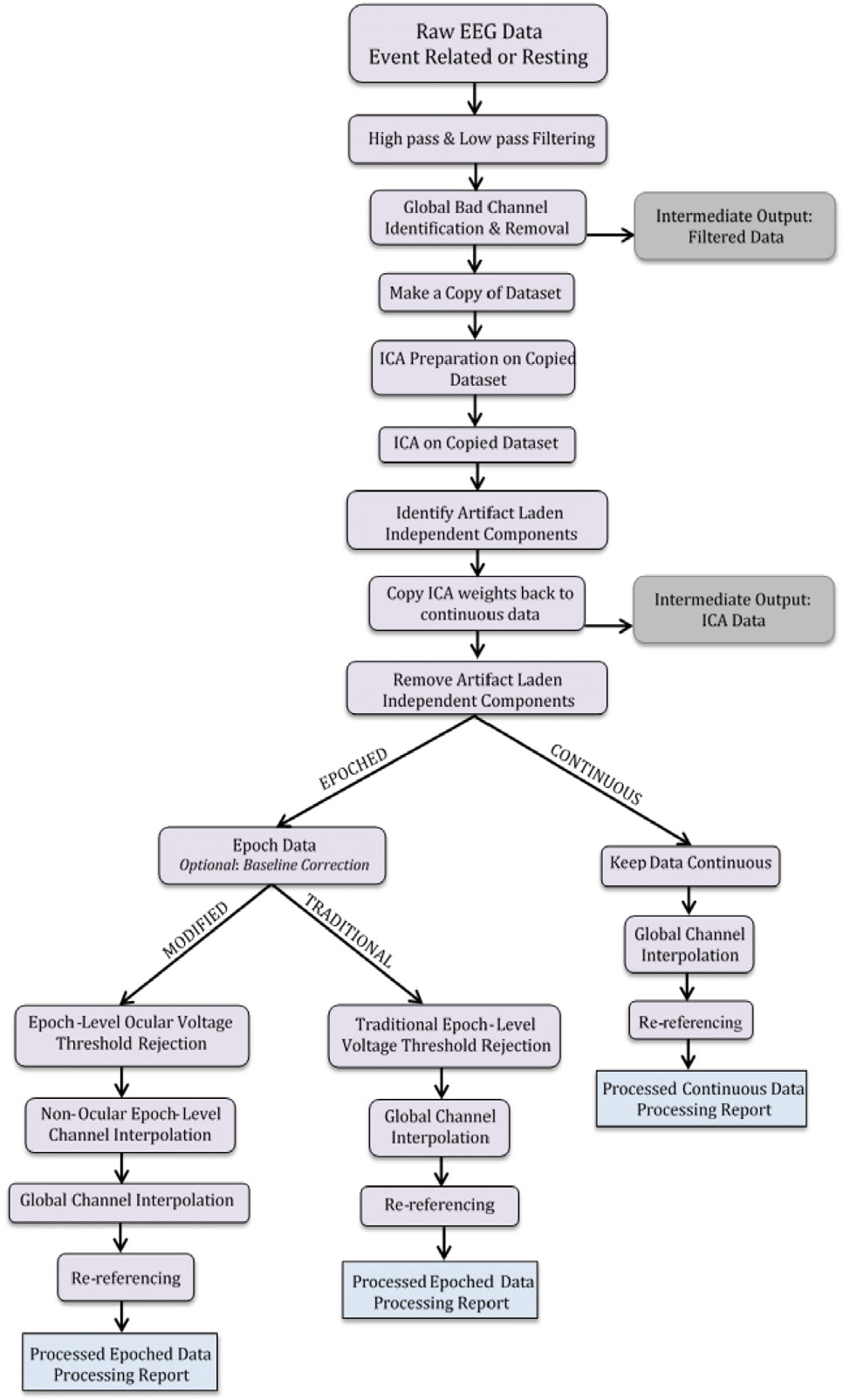
MADE preprocessing pipeline [48]. Permission granted by Wiley Online Library.

Secondly, HAPPE starts with high-pass (1 Hz) and low-pass filtering (250 Hz) (Figure 2). Then, it allows the researcher to select the channels that he/she wishes to analyze based on the 10-20 International system (plus more if needed). In fact, performing channel reduction from the 128 channels is recommended for better ICA performance as high-density EEG along with short length of recording (which infants often have) compromises the stability and robustness of ICA. Next, the electrical line noise is removed via the multi-taper regression function of the CleanLine program [83], while automated bad channel (more than 3 standard deviation (SD) from the mean) detection is performed twice.

Fig. 2

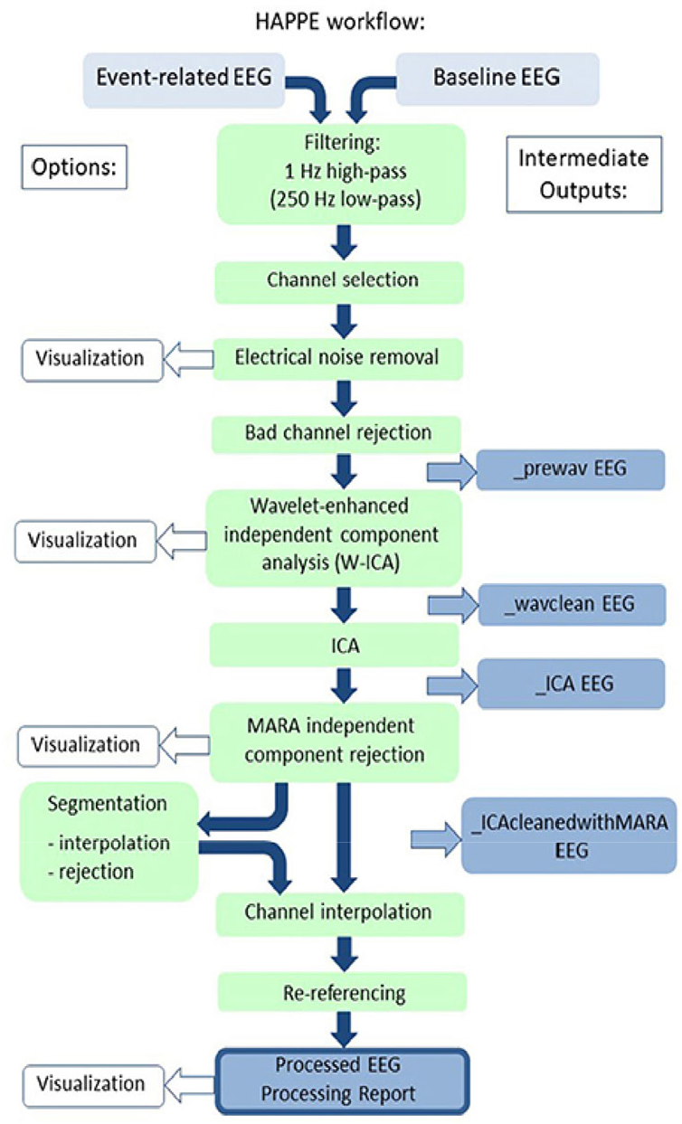
HAPPE preprocessing pipeline [47]. Under Creative Commons Licence (CC BY) (https://creativecommons.org/licenses/by/4.0/) by Frontiers.

Furthermore, W-ICA is performed for the detection of gross artifacts, such as high-amplitude signals and signal discontinuations, and the differentiation between good and artifactual ICs. After W-ICA, HAPPE continues with ICA decomposition, via the extended Infomax algorithm, for the residual artifacts, while the rejection of the artifactual ICs is performed via MARA. Interestingly, it has been argued that an initial W-ICA leads to better ICA results. Next, epoching and post-segmentation artifact correction are optional steps. In fact, there are two post-segmentation artifact correction options depending from the recording length. Specifically, in short recordings, interpolation is completed via FASTER, while for longer recordings it is proposed to reject bad segments from the entire or designated channels, based on the criteria of amplitude and probability. Finally, HAPPE finishes with interpolation via spherical spline and re-reference (average or otherwise).

Notably, the creators of HAPPE expanded the pipeline for low-density EEG recording (HAPPE In Low Electrode Electroencephalography (HAPPILEE) [84], and they tested it in the pediatric population of the previous dataset.

Thirdly, APICE allows various procedures and actions with the creation of four different pipelines; APICEa (skips the in-depth artifact correction process), APICE, APICE + W-ICA and APICE + Denoising Source Separation (DSS) for Event-Related Potentials (ERPs) (Figure 3). Its basic steps are as follows; high-pass (0.1 Hz) and low-pass filtering (40 Hz), artifact detection/ correction/rejection, define bad sample and channels, target principal component analysis (PCA), define bad sample and channels, spherical spline interpolation of channels with short bad times, W-ICA with iMARA (optional), whole-channel spherical spline interpolation, artifact detection/correction/detection, define bad sample and channels, epoching, bad epoch detection, whole-channel spherical spline interpolation, bad epoch rejection, DSS (optional), AR, baseline correction (optional). Notably, the authors mentioned that the implementation of ICA and DSS slightly improves the quality of the dataset.

Fig. 3

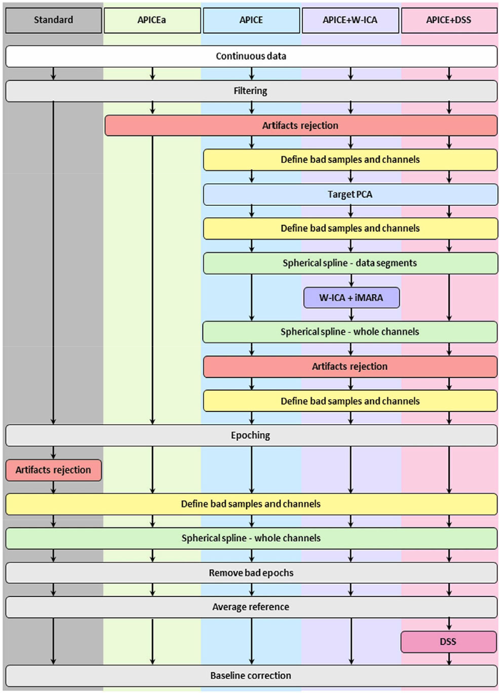
APICE preprocessing pipeline [49]. Under a Creative Commons Licence (CC-BY-NC-ND) (https://creativecommons.org/licenses/by-nc-nd/4.0/). Permission granted by Elsevier.

Interestingly, its artifact correction procedure is quite complex. In particular, for the artifact detection and correction process, the pipeline uses multiple algorithms with flexible adaptive thresholds based on the specific electrodes, the age of the subject, the EEG condition (resting or active state). In fact, it goes twice through 5 different cycles, using algorithms which are responsible for different types of artifacts e.g. compute channel correlation to find bad channels, use of absolute thresholds to reject data with excessive high amplitude and use of relative thresholds (based on amplitude, variance, running average, discontinuities, rapid signal change) to detect motor artifacts. Next, target PCA is performed for the correction of transient artifacts, such as signal discontinuities, in those specific segments that have been labeled as artifactual. Also, bad epoch is defined based on three parameters; as the segment with any bad time, if it contains 30% of bad channels and if more than 50% of its content has been interpolated.

It is worth mentioning that APICE differentiates between “Bad Times” and “Bad Channels”, with the former being salvageable. Bad channels in the continuous data are those which are bad for more than 30% of the time, whereas in the segmented data are those with more than 100 ms of “badness” within one epoch.

Lastly, we decided to include recommendations regarding preprocessing that precedes FC analysis. Firstly, high-pass filtering is not recommended as it can bring dependencies between adjacent data samples [85], compromising the true neural connectivity measurement. Detrending methods, such as piecewise detrending, have been proposed as an alternative to high-pass filtering [85, 86]. Secondly, fixed-length epochs are considered more appropriate for FC analysis [87] with 4-second segmentation being suggested as the basis as it provides stability [18, 88]. Bastos & Schoffelen [34] mentioned that short epochs should be avoided as they can lead to connectivity bias. It should be noted that various epoch-lengths have been recommended for FC analysis depending from the method that is employed. For example, it has been mentioned that 6-second epoching is a good choice for amplitude envelope correlation while 12-second epoching for PLI [18]. Thirdly, automated instead of manual procedures have been suggested for artifact correction when computing FC as connectivity bias is decreased. Nevertheless, the appropriateness of automated procedures for FC analysis is not always supported [89].

Fourth, there have been studies which investigated the appropriateness of different types of re-reference for FC analysis. Kayser and Tenke [90] highlighted that a single reference is not suitable for this type of processing as a commonality may appear in all electrodes, compromising the true neural connectivity between the electrodes [91, 92]. Chella et al. [91] reported that linked mastoids (LM) reference was also deemed not appropriate for connectivity analysis, as some studies have found that these areas may not be as separate from brain activity as commonly thought [18]. Also, they found that vertex (Cz) reference lead to the biggest distortions of the EEG data. In contrast, several recent and older studies have reported that Reference Electrode Standardization Technique (REST) and (common) average reference (AR) are the best choice for FC analysis [18, 91, 93] with the former being the most suitable as it provides the most objective measurements. AR is considered the closest resemblance of REST, leading to less EEG signal distortions than any other reference such as Cz or mastoids. In fact, AR is considered the most appropriate type of re-referencing when computing coherence [94], with high-density EEG recording reportedly increasing the effectiveness of AR [95, 96] and dropping the error of connectivity values below 10% [97]. However, as argued by Smith et al. [98], the small head of infants provides extensive scalp coverage regardless of electrode density, making the choice of a specific re-reference less important in certain linear FC metrics, such as cross-correlation. Finally, (surface) Laplacian or current source density (CSD) is a re-reference free montage [99] and has been shown to be effective in associating behavior and EEG signal in two neonatal studies [60, 100].

4 Processing

4.1 Coherence and CFC

FC analysis proceeds preprocessing, with several existing methods offering either linear and non-linear connectivity measurement. There are several reviews and studies in literature that have described and compared the advantages and disadvantages of these methods. For example, Bastos and Schoffelen [34], and Wang et al. [101] reviewed several variations of coherence metrics (i.e. ordinary coherence, slope of the phase difference spectrum, PSI, imaginary coherence and PLV), Sakkalis [102] compared the basic linear metrics with non-linear ones, Bakhshayesh et al. [103] compared 26 FC metrics such as coherence, mean-phase coherence, mutual information (kernel) etc, Hindriks [104] compared PLI with lagged coherence, and Hülsemann et al. [105] reviewed some of the methods for CFC calculation. All metrics have their pros and cons, and each of them performs better at one aspect and bad in another one.

The current study focuses mostly on the traditional type of coherence (i.e. ordinary coherence) and the CFC metrics that have been applied in infantile FC studies. Interestingly, it has been suggested that both of them are produced by the same neural network mechanisms [106].

Firstly, coherence was initially proposed by Goodman in 1960 [107] and is based on a bivariate (electrode-to-electrode) autoregressive model computing the time-domain correlation between two signals [108–110], with 1 indicating synchronization and functional communication between the underlying areas and 0 the lack of inter-areal coordination [111, 106]. In plain language, coherence measures the statistical relation between the power spectra of two signals, as recorded by two different channels, revealing their phase synchrony. It requires first performing spectral analysis using wavelet decomposition methods, such as fast Fourier transformation (FFT) or the Welch’s method [112]. An interesting older review discussed the relationship and commonness between coherence and correlation calculation [113]. In fact, it is worth noting that coherence does not simply reflect Pearson correlation but the frequency-dependent squared cross-correlation. Nevertheless, the disadvantages of this metric have also been addressed by a recent review [114].

There are two reported equations in literature for the calculation of the two main types of coherence, i.e. complex (1) and ordinary coherence (2), with the latter being the magnitude squared of complex coherence and the most common in research [111].

$C\chi y(\omega )=\frac{S\chi y(\omega )}{\sqrt{S\chi \chi (\omega )Syy(\omega )}}$

1

$G^2\chi y(\omega )=\frac{{|S\chi y(\omega )|}^2}{S\chi \chi (\omega )Syy(\omega )}$

2

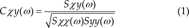
with: a) Sxx(ω) = power spectral density of x

b) Syy(ω) = power spectral density of y

c) Sxy(ω) = cross-spectral density of xy

Volume conduction is one of the major issues when computing coherence, often leading to increased false-positive coherence values [112, 115]. Specifically, it refers to the tendency of the electrodes to pick up the activity of nearby areas and is related to the low-spatial resolution of the EEG. One countermeasure is to calculate the imaginary [116] and not the absolute value of coherence or to apply an inverse solution and construct a source model. This problem has prompted numerous researchers to try and develop novel coherence metrics that could potentially minimize the effect of volume conduction such as the partial coherence field [117], coherence with CSD [118], isolated effective coherence [119] and reduced coherence [97]. Another limitation that is posed by coherence analysis is the fact that it requires relative lengthy epochs, as short ones can create biases when it comes to signal connection. Notably, False Discovery Rate (FDR) is an algorithm used to decrease the chance of finding false-positive brain connectivity values by applying a specific threshold usually at 1%, 5% or 10% [120]. Finally, coherence can be influenced by both phase and amplitude changes and thus it is unclear whether this metric reflects phase or amplitude interactions, or both [45].

Moreover, CFC refers to the coupling of a slow frequency with a faster one [121, 122] (S-F coupling) and it can be divided into phase-phase coupling (PPC), phase-amplitude coupling (PAC) and ampitude-amplitude coupling (AAC or CFS). Specifically, S-F coupling indicates the non-linear communication between distributed brain networks and has been associated with higher cognitive functions such as information processing, attention, learning and memory [5, 122, 123]. Interestingly, it has been argued that the structural base which supports CFC, i.e. thalamo-cortical and cortico-cortical networks, is present from the third trimester of pregnancy [124, 125]. In fact, several neonatal studies managed to successfully demonstrate that PAC can be present from birth [57, 126–130], possibly indicating brain maturation including myelination and information processing. It’s important to highlight that the choice of the most suitable CFC metric for investigating brain network communication remains a subject of ongoing debatebecause there is supporting evidence for all three options [5, 34]. Nevertheless, during the last decade, CFC analysis has gained popularity for the measurement of the non-linear local and widespread network communication in the young brain. However, till this day only a few studies have employed it in infants.

Interestingly, both linear and non-linear methods can be applied for the computation of CFC; cross-correlation, envelope to signal correlation (ESC) [131], PLV, mean vector length (MVL) [132], general linear model measure (GLM) [133], amplitude power spectral density (APSD) [134], coherence value (CV) [135], modulation index (MI) [136], event related phase amplitude coupling (ERPAC) [137] and mutual information for phase-amplitude coupling (MI-PAC) [138]. Notably, in many studies that calculate PAC, researchers first perform Hilbert transformation (complex demodulation) to obtain the phase and amplitude values of the sinusoidal waves, and then they continue with the application of coupling method [128–130, 139].

Next, we present some of the limitations of CFC metrics. In particular, ESC has the disadvantage to be sensitive to coupling phase and less effective in measuring coupling intensity [140]. The latter limitation also concerns PLV, GLM, APSD, CV and ERPAC. Then, MVL and MI require lengthy data in order to have good result. In addition, only MI and GLM can measure biphasic coupling with the former being suggested for short and noisy data, while the latter for lengthy and clean data [105]. Also, the reader should keep in mind that ERPAC is for FC analysis of ERPs [140].

Many of the coherence and CFC metrics can be applied in MATLAB and EEGLAB with already embedded functions (e.g. coherence, partial coherence, imaginary part of coherency, PLV, cross-correlation) or additional toolboxes such as PACTools [141] that computes MVL, MI, PLV, GLM and MI PAC, and MNE-Python (e.g. coherence, partial directed coherence, imaginary part of coherency, cross-correlation, PSI, ESC). Other common MATLAB toolboxes for EEG analysis is Brainstorm [142] and Fieldtrip [143]. Also, EEG Analysis System (James Long Company, NY, USA) is another popular software for the same purpose.

4.2 Coherence and CFC application in infant studies

Coherence analysis has been performed in typical infants and toddlers for the study of language [41, 144], inhibition [42, 145–147], motor-skills [67, 148–150], working-memory [26, 65, 146, 151–153], attention [144, 145, 154]. In addition, it has been applied in infants at-risk for ASD [155, 156], preterm [95, 148, 157] and with extremely low-birth weight [158]. It should be noted that several of these studies measured and/or the sleep state of the individuals [95, 157–159].

As we can see in Table 1, the above (ordinary) coherence studies used different recording, preprocessing and processing procedures.

Table 1

Coherence studies

Articles	EEG bands of interest	Areas of interest	Length of data	Epoch Length	High- and low-pass filtering	Artifact correction process	Software/FC analysis
Kühn-Popp et al. [41]	alpha (6–9 Hz)	Frontal-central and frontal-occipital	Baseline: 3 pre-cleaned min/2.5 cleaned minutes	1024 ms with 50% overlap	0.1–20 Hz	Manual and semi-automated post-segmentation procedures: for eye and motor artifacts → visual inspection and automated artifact rejection if their amplitude exceeded ±120μV the mean amplitude and by setting minimal-maximal difference at ±100 μV	Coherence correlation application in the Vision Analyzer software
Tran et al. [155]	theta(4–6 Hz), alpha(6–12 Hz)	Fronto-temporal, fronto-central	Active state:2.5 pre-cleaned min/87 cleaned secconds	3 s	1.5–50 Hz	Semi-automated pre-segmetation procedures: a) for gross artifacts → perform artifact subspace reconstruction and infinite impulse response spectral weighting and reject data if exceeded SD by 8, b) for bad channels → reject channels if had more than 3-sec of flat-line or had less than 0.75 correlation with other channels, c) for eye, motor and heart beat artifacts → perform Adaptive Mixture ICA (AMICA) [160] + manual removal of bad ICs	Coherence analysis in MATLAB/ EEGLAB via the newcrossf function
Righi et al. [156]	gamma (30–50 Hz)	Frontal and temporo-parietal	Baseline: aproximately 5 pre-cleaned min ± 1.5 min + Active state: 3 pre-cleaned min/cleaned lengths not mentioned	Not mentioned	0.1–100 Hz + notch filter at 58–62 Hz	Automated procedures: reject data if exceeded ± 200 μV the mean data or if more than 10% of the segments were bad	Coherence analysis in MATLAB/ EEGLAB via the newcrossf function
Myers et al. [95]	0–3, 4–6, 7–9, 10–12, 12–14, 15–17, 18–20, 21–23 , 24–36,37–48 Hz	All brain areas	Sleep state:1 pre-cleaned hour/at least 3 cleaned min	30 seconds	0.1 to 400 Hz + notch filter at 60 Hz	Automated post segmentation procedures: a) for individual bad data → reject if exceeded SD by 50 μV, b) for bad epochs → reject if channels exceeded SD by 25%	Coherence analysis with FDR at 10% in MATLAB
Grieve et al. [158]	delta (1–4 Hz), theta(4–8 Hz), alpha (8–12 Hz), beta (12–24 Hz), low gamma (24–40 Hz), gamma (40–50 Hz)	All brain areas	Sleep state: pre-cleaned length not mentioned/5.5 ± 2.85 cleaned min for full-term, 11.3 ± 9.2 cleaned min for preterm infants	30 seconds	0.1 to 400 Hz + notch filter at main frequency powers	Automated pre-segmentation procedures: see Grieve et al. [159]	Average coherence of all electrodes with FDR at 5% in MATLAB
Grieve et al. [159]	6, 10, 18 Hz	All brain areas	Sleep state: pre-cleaned length not mentioned/2 cleaned min	1 second	1–400 Hz	Automated pre-segmentation procedures: for bad channels → reject data if exceeded SD by 50 μV	Spatial signal correlation and coherence analysis in MATLAB after making a head model from a single cortical current dipole
Whedon et al. [145]	alpha(6–9 Hz)	Frontal polar, medial and lateral frontal	Baseline: lengths not mentioned	Not mentioned	0.1–100 Hz	Automated procedures: a) for eye artifacts → identification based on the peak-to-peak criterion at ≥50 μV, b) for motor artifacts → identification based on the peak-to-peak criterion at >200 μV} reject segments if artifact scored	Coherence analysis in the EEG Analysis System via the algorithm by Saltzberg et al. [161]
Xiao et al. [67]	alpha (6–9 Hz)	Frontal, motor, and parietal	Baseline: at least 80-120 pre-cleaned sec/cleaned length not mentioned + Active State: 200 pre-cleaned and cleaned sec	Not mentioned	0.3–30 Hz	Semi-automated procedure: a) for bad segments→ visual inspection and rejection, b) for bad electrodes → rejection if their kurtosis exceeded SD by 5, c) for eye and motor artifacts → ICA+ manual rejection of bad ICs	Coherence analysis in MATLAB/ EEGLAB via the mscohere function
Nishiyori et al. [148]	alpha band (6–9 Hz)	Frontal, motor, and parietal	Baseline: 2 pre-cleaned min + Active state: 180 pre-cleaned sec/less than 47.6 ± 22.3 cleaned sec (unclear whether for both EEG conditions or just one)	Not mentioned	0.3–30 Hz	Semi-automated procedure: a) for bad segments→ visual inspection and rejection, b) for bad electrodes rejection if their kurtosis exceeded SD by 5, c) for eye and motor artifacts → ICA+ manual rejection of bad ICs	Coherence analysis in MATLAB/ EEGLAB via the mscohere function
Broomell et al. [42]	alpha (6–9 Hz)	Fronto-temporal	Baseline: 1 pre-cleaned min/42 cleaned sec	Not mentioned	0.1–100 Hz	Automated procedures: a) for eye artifacts → identification based on the peak-to-peak criterion at ≥100 μV, b) for motor artifacts → identification based on the peak-to-peak criterion at >200 μV} reject segments if artifact scored	Coherence analysis in the EEG Analysis System via the algorithm by Saltzberg et al.
Corbetta et al. [150]	alpha (6–9 Hz)	Lateral frontal and central sites	Baseline: 1 pre-cleaned min + Active state: 5-5.5 pre-cleaned min/cleaned lengths not mentioned	Not mentioned	0.1–100 Hz	Automated procedures: a) for eye artifacts → identification based on the peak-to-peak criterion at ≥100 μV, b) for motor artifacts → identification based on the peak-to-peak criterion at >200 μV } reject segments if artifact scored	Coherence analysis in the EEG Analysis System via the algorithm by Saltzberg et al. (equation 9)
Mundy et al. [144]	theta (4–6 Hz)	Frontal -central, frontal-occipital	Baseline: 3 pre-cleaned min/ cleaned length not mentioned	Not mentioned	1–100 Hz + notch filter at 60 Hz	Semi-automated procedures: a) gross motor artifacts → visual inspection and rejection, b) for eye and motor artifacts → reject data based on the average data scoring	Coherence analysis in the EEG Analysis System via the algorithm by Saltzberg et al.
Bell & Fox [151]	alpha band (6–9 Hz)	Frontal-parietal, frontal-occipital	Baseline: 2 pre-cleaned min/90 cleaned sec	30 seconds	1–100 Hz	Automated post-segmentational procedures: for eye artifacts → reject data based on the scoring using the signal from Fp1 and Fp2	Coherence analysis in the EEG Analysis System via the algorithm by Saltzberg et al.
Bell & Fox [149]	alpha (6–9 Hz)	Medial frontal/ parietal, medial frontal/ occipital, lateral frontal/ parieta1, lateral frontal/occipital, parietal/ occipital	Baseline: 3 pre-cleaned min/ cleaned length not mentioned	Not mentioned	1–100 Hz + notch filter at 60 Hz	Automated procedures: for eye and motor artifacts → reject data based on the average data scoring	Coherence analysis in the EEG Analysis System via the algorithm by Saltzberg et al.
Bell [146]	alpha (6–9 Hz)	frontal pole, medial frontal, lateral frontal, parietal, occipital	Baseline: 1 pre-cleaned min + Active state: pre-cleaned length not mentioned/ cleaned length not mentioned	Not mentioned	1–100 Hz	Automated procedures: a) for eye artifacts → identification based on the peak-to-peak criterion at ≥100 μV, b) for motor artifacts → identification based on the peak-to-peak criterion at >200 μV } reject segments if artifact scored	Coherence analysis in the EEG Analysis System via the algorithm by Saltzberg et al.
Bell & Wolfe [152]	alpha (6-9 Hz)	Medial frontal with all other electrode sites	Baseline: 1 pre-cleaned min/ cleaned length not mentioned + Active state: lengths not mentioned	Not mentioned	1–100 Hz	Semi-automated: a) for eye artifacts → identification based on visual inspection and the peak-to-peak criterion at ≥100 μV b) for motor artifacts → identification based on the peak-to-peak criterion at >200 μV } reject segments if artifact scored	Coherence analysis in the EEG Analysis System via the algorithm by Saltzberg et al.
Cuevas et al. [147]	alpha (6-9 Hz)	Medial frontal–all other electrode sites	Active state: lengths not mentioned	Not mentioned	0.1–100 Hz	Automated procedures: a) for eye artifacts → identification via scoring using the signal from Fp1 and Fp2, b) scoring for gross motor artifacts, c) scoring for hear beat artifacts } reject segments if artifact scored	Coherence analysis in the EEG Analysis System via the algorithm by Saltzberg et al.
Cuevas et al. [153]	theta (1.5–5.5 Hz), alpha (5.5–9.5 Hz), beta 1 (9.5–13.5 Hz)	Frontal-parietal, frontal-temporal, frontal-occipital	Baseline: 1 pre-cleaned min/ cleaned length not mentioned + Active state: lengths not mentioned	Not mentioned	0.1–100 Hz	Automated procedures: a) for eye artifacts → identification based on the peak-to-peak criterion at ≥100 μV, b) for motor artifacts → identification based on the peak-to-peak criterion at >200 μV } reject segments if artifact scored	Coherence analysis in the EEG Analysis System via the algorithm by Saltzberg et al.
Cuevas et al. [65] + Cuevas & Bell [26]	alpha (6–9 Hz)	Medial frontal–all other electrode sites	Baseline: 1 pre-cleaned min/ cleaned length not mentioned + Active state: lengths not mentioned	Not mentioned	0.1–100 Hz	Automated procedures: a) for eye artifacts → identification via scoring using the signal from Fp1 and Fp2, b) scoring for gross motor artifacts, c) scoring for hear beat artifacts } reject segments if artifact scored	Coherence analysis in the EEG Analysis System via the algorithm by Saltzberg et al.
Duffy et al. [157]	0.5–32 Hz	All brain areas	Sleep state: pre-cleaned length not mentioned/ less than 15.4 ± 3.13 cleaned min	2 seconds	1–90 Hz	Semi-automated pre-segmentation procedures: a) visual inspection and rejection of bad epochs, b) for motor artifacts → automated rejection of data above 32 Hz	Coherence analysis in the Nicolet software via the algorithm by Saltzberg et al.

High-density recording (≥124 electrodes) was performed by five of the above studies [95, 155, 156, 158, 159], with two of them [155, 156] significantly reducing the number of electrodes to just twelve during data analysis. The rest of the studies performed an initial low-density recording (≤32 electrodes) while analyzing an even smaller amount of electrodes (i.e. ≤20). Next, all of the above studies performed AR except Tran et al. [155] and Duffy et al. [157] who applied CSD. Also, for spectral analysis, FFT [41, 95, 158, 159], Welsch’s method [67, 148, 155], discrete Fourier transform [26, 42, 65, 144–147, 149–153] and Morlet wavelet transform [156] were chosen.

Other type of linear connectivity metrics have been employed in infantile EEG studies, such as the imaginary part of coherency [162], cross-correlation [163], weighted PLI (wPLI) and/or PLI [88, 164, 165], but these are beyond the scope of the current review.

Next, CFC has been employed to demonstrate the development of the infantile neural networks in the typical [57, 60, 128, 139] and atypical brain (i.e. infants with encephalopathy or premature birth) [126, 127, 129, 130]. It’s worth noting that Tokariev [60], Moghimi [127], and Witte [139], along with their colleagues measured the brain activity during quiet and/or active sleep.

Much like in coherence studies, these CFC studies also applied different recording, preprocessing and processing techniques. Firstly, low-density (<20 electrodes) [60, 126, 127, 129, 130, 139] and high-density EEG recording (>65 electrodes) [57, 128] was performed. Secondly, the majority of them measured PAC across all electrodes and brain sites, except Tokariev et al. [60] who calculated all three CFC metrics. Third, all researchers chose to focus on different EEG bands. In particular, for the slower waves, frequencies such as 0.7–2 Hz [57], 0.75–3 Hz [139], 1–2 Hz [129, 130], 0.5–1.5 Hz [126], 0.5–2.5 Hz [127] and 2-8 Hz [128] were selected, while for the faster activity the researchers chose 11.3–32 Hz, 3–12 Hz, 12–30 Hz, 8-25 Hz, 4–7.5 Hz and 15– 45 Hz respectively. Interestingly, Tokariev et al. [60] measured S-F coupling between multiple frequency pairs; 0.7, 1.0, 1.4, 2.0, 2.8, 4.0, 5.7, 8.0, 11.3, 16.0, 22.6, and 32.0 Hz. Fourth, all of them performed AR except Tokariev et al. [60] and Shibata & Otsubo [126] who chose CSD and single electrode reference (Cz or Pz) respectively.

One of the main differences between the preprocessing applied by the CFC and coherence studies is that the former performs an additional filtering on the specific EEG bands of interest, while spectral analysis can often be omitted if the (absolute or relative) power calculation is not the goal of the study (only Attaheri et al. [128] and Witte et al. [139] performed one). Below, we delineate the details of the preprocessing and processing techniques (Table 2).

Table 2.

CFC studies

Articles	Length of data	Filtering	EpochLength	Artifact Correctionprocedure	CFC metric	FC method and software
Attaheriet al. [128]	Baseline:5 pre-cleaned min/ cleaned length not mentioned + Active state: 20.33 pre-cleaned min/5.5 cleaned min	First: 0.5–45 Hz + Second: 2-8 Hz, 15–45 Hz	4.23 seconds ± 0.88-seconds	Automated pre-segmentation procedures: a) for noise artifacts → modified PCA, b) for bad channels → identified via probability + kurtosis criterion and interpolated + Automated post-segmentation procedures: a) for bad channels → identified via probability + kurtosis criterion and interpolated,b) reject epochs if exceeded1000 μV or 3 SD from the mean	PAC	MI via WinPACT in MATLAB/ EEGLAB
Tokarievet al. [60]	Sleep state: 20 pre-cleand andcleaned min	First: not mentioned + Second: Set ofinto 13 EEG bands filters with central frequencies: 0.5, 0.7, 1, 1.4, 2, 2.8,4, 5.7, 8, 11.3, 16, 22.6, 32 Hz	5 minutes	Manual pre-segmentation procedures: visual inspection and choose the least noisy segments	PAC, AAC, PPC	PLV (for PAC + PPC) and cross-correlation (for AAC) in MATLAB and Labview [166]
Moghimiet al. [127]	Quiet sleep state:15 pre-cleaned min/ cleaned length not mentioned + Sleep state with auditory stimulus: pre-cleaned length not mentioned/ 45.15 ± 4.93 cleaned min (7 min were used for PAC)	First: 0.5–20 Hz+ Second: 0.5–2.5, 4–7.5 Hz + Third: 1.5–10, 3–20 Hz	14 seconds	Automated pre-segmentation procedures: reject data if amplitude exceeded 5 SD from the mean	PAC	Synchronization index (measures locking strength) (with second filtering) + MI (with third filtering) in MATLAB
Shibata & Otsubo [126]	Unclear whether awake or sleep state: 6-28 pre-cleaned min/upto 6 cleaned min	No filter	2 minutes	Manual pre-segmentation procedures: visual inspection and choose the least noisy segments + Post-segmentation (does not mention manual or automated): rejection of heart beat and motor artifacts	PAC	MI + direct MVL via PACT in MATLAB/EEGLAB
Witteet al. [139]	Sleep state:3 pre-cleaned hours/80 s	Not mentioned (except for the second filter for the high frequency at 3–12 Hz)	4 seconds	Manual pre-segmentation procedures: visual inspection and choose the epochs that contained burst patterns	Phase synchrony + PAC	Bispectral analysis + amplitude envelope correlation (software not mentioned)
Wanget al. [130]	Sleep state:6 pre-cleanedhours/at least30 cleaned min	First: 0.5-70 Hz + notch filter at 60 and 47 Hz + Second: 1–2 Hz, 12–30 Hz	1 second	Automated post-segmentation procedures: a) for motor artifacts → reject epochs if exceeded 50 μV or less than3 μV from the meanb) for bad channels → reject if amplitude exceeded 4 SD the mean data	PAC	MVL in MATLAB
Marischalet al. [57]	Baseline:5 pre-cleaned min/1 cleaned min	First: 1-100 Hz + Second: 2–20 Hz, 40-100 Hz	2 seconds	Automated pre-and post-segmentation procedures: via HAPPE pipeline	PAC	MI and phase-max via PACTtools in BEAPP [167]

4.3 Graph theory analysis

Generally, a “graph” refers to the visual depiction of a network that is comprised by nodes (i.e. vertices) and edges (i.e. connections) [46]. A node is defined by the spatial position of the EEG electrodes [168], while an edge represents the temporal correlation or coherence between the signals [169, 170]. Graphs can be divided into four categories; weighted directed, unweighted directed, weighted undirected and unweighted undirected [171]. Usually, weighted directed graphs provide more information about networks than the others. Also, connection metrics can be shown in the form of adjacency or connectivity matrices with the latter being a broader term than the former one.

There are several types of graph theory measures, with some of the basic general categories being degree, strength, cluster coefficient, path length, modularity, small-worldness etc [172].

Then, graph theory analysis is divided into four steps; a) determine network nodes via electrode array or MRI data, b) measure the linkage between nodes e.g. via coherence, c) create a correlation matrix (i.e. adjacency matrix or undirected graph) by setting firstly a connection threshold, then taking all the pairwise correlations between nodes, d) compute the graph measures of interest and compare them with other random networks.

Specifically, connectivity thresholds of the edge densities between the nodes can be either absolute (i.e. setting an absolute correlation limit to what will be considered significant connection) or proportional (i.e. finding the strongest threshold of each participant while keeping the number of connections fixed for all them) with the latter approach leading to homogeneity across the graph networks of the group and to more stable networks [33, 173]. Nevertheless, it has been argued that proportional thresholding increases the risk of finding random connections in case of low pre-existing FC.

The recommended lower cut-off point by several adult [174, 175] and infantile studies [7, 33, 62, 98] when performing graph theory analysis is between 0.1-0.5. It should be mentioned that thresholding could be skipped when calculating for example weighted graphs and measures, such as the weighted degree [98, 171]. However, there is still not a general consensus regarding the specific threshold values, with many studies performing different ones [176].

Interestingly, it should be mentioned that high-density EEG recording is associated with elevated numbers of calculated nodes and improved network accuracy [177].

For further information on graph theory analysis see the reviews by Bullmore and Sporns [171], Farahani et al. [46] while Zhao et al. [68] provide a comprehensive review on graph theory analysis in the infantile population.

Moreover, graph theory analysis has increasingly accompanied linear and non-linear FC EEG studies. This integration is used to explore and visualize the evolving architecture of neural networks in both healthy term [7, 33, 62, 89, 98, 178–180] and preterm infants [179, 181].

Similarly in the coherence and CFC studies, researchers applied different recording, preprocessing and processing procedures in this type of analysis. Firstly, most of them performed low-density electrode recording and processing (<20 electrodes) [33, 62, 89, 98, 181], except Rotem-Kohavi et al. [180] who recorded and processed 64 electrodes, Omidvarnia et al. [179] who recorded 28–64 channels and processed 25 of them, and Xie et al. [7] who recorded 128 electrodes and processed 126. The recording was performed on awake [7, 180] and/or sleeping infants [33, 62, 89, 98, 179], while Hendrikx et al. [181] used one-channel EEG (C3–C4) on sedated infants. Next, they performed automated or semi-automated artifact correction procedure on epoched [7, 33, 62, 98] or continuous data [179–181], except Bosch-Bayard et al. [89], who visually inspected and chose the least noisy epochs. Artifact correction procedure on the epoched data was either pre-segmentational [62, 89], post-segmentational [7, 33], or both [98] and were similar with those of coherence and CFC studies. Epoch lengths were composed by 1.00 s [7, 62, 98], 2.00 s [62], 2.56 s [89], or 4.00 s [33]. Also, all of them performed AR except Omidvarnia et al. [179] who applied CSD.

As we will see below, for the FC calculation, the researchers employed wPLI, partial coherence, cross-correlation or PLI. The last two are linear FC metrics while the first and some variations of the second are reportedly able to compute both linear and non-linear signal interactions [182–184]. On Table 3 below we provide more information about the specifics of their graph theory analysis.

Table 3.

Graph theory studies

Articles	Length of data	Frequencies of interest	FC calculation tool	Graph analysis measures	Type of graph and/or matrix + connectivity threshold(if applied)	Software and toolbox or algorithm for graph analysis	Source localization procedure
Rotem-Kohaviet al. [180]	Baseline: 30 pre-cleaned sec + Active state:90 pre-cleaned sec / cleaned lengths not mentioned	4–40 Hz	FDR controlled PC algorithm (PCFDR) [120] + FDR at 5%	1) characteristic path length2) density2) global efficiency3) modularity	Undirected graph (threshold not mentioned)	MATLAB/Brain Connectivity Toolbox [185]	-
Tóthet al. [33]	Sleep state: 5 pre-cleaned min/ 140 cleaned seconds	Delta: 0.5–4 Hz, theta: 4–8 Hz, lower alpha: 8–10 Hz, upper alpha: 10–12 Hz, beta: 13–30 Hz, gamma: 30–45 Hz	PLI	1) maximal degree, 2) maximal betweenness centrality,3) leaf fraction,4) diameter,5) tree hierarchy	Undirected weighted graph + proportional thresholding	BrainWave software/ Kruskal’s Minimum spanning tree (MST) algorithm [186]	-
Hendrikxs et al. [181]	Awake state:5 pre-cleaned min/ cleaned length not mentioned + Sedated state: 10 pre-cleaned hours/ 6 cleaned hours	Not mentioned	Cross-correlation	1) vertex degree,2) global degree	Undirected weighted graph + adjacency matrix (thresholding not mentioned)	MATLAB/toolbox for network analysis provided by MIT Strategic Engineering	-
Smithet al. [98]	Mixture of awake and sleep state: 20.8 pre-and post-cleaned hours	0.5–55 Hz	Cross-correlation	1) degree2) clustering coefficient,3) shortest path length	Weighted graph + adjacency matrix + proportional thresholding	Software not mentioned	-
Hu et al. [62]	Mixture of awake and sleep state: 20-70 pre-cleaned min/Awake state: 240 cleaned sec + Sleep state: 240 cleaned seconds	Delta (2–4 Hz), theta (4.5–7.5 Hz), alpha (8–12.5 Hz), and beta(13–30 Hz)	Cross-correlation + wPLI	1) network strength,2) normalized normalized global clustering coefficient,3) normalized characteristic path length length,4) small-worldness	Weighted adjacency matrix + absolute thresholding	MATLAB/Brain Connectivity Toolbox	-
Omidvaria et al. [179]	Sleep state: Pre-cleaned length not mentioned/5 cleaned minutes	Theta(3-8 Hz), alpha(8-15 Hz)	Orthogonalized envelope correlation [187] + FDR at 1%	1) clustering coefficient,2) characteristic path length,3) modularity,4) small-worldness	Weighted graphs + adjacency matrix + binary thresholding	MATLAB/Brain Connectivity Toolbox	-
Xie et al. [7]	Active state: 10-15 pre-cleaned min/at least 200± 40 cleaned seconds	Theta (2–6 Hz), alpha (6–9 Hz), beta (9–13 Hz)	wPLI + FDR at 5%	1) path length,2) clustering coefficient,3) small-worldness	Adjacency matrix + proportional thresholding	MATLAB/Brain Connectivity Toolbox and GRETNA toolbox [188]	FEM model + eLORETA [189] in MATLAB/ Fieldtrip toolbox
Bosch-Bayard et al. [89]	Sleep state: Pre-cleaned length not mentioned / 61.44 cleaned seconds	Delta (1–4 Hz), theta (4–8 Hz), alpha (8–12 Hz), beta 1 (12–20 Hz), beta 2 (20–30 Hz)	Isolated effective coherence + FDR at 5%	1) eigenvector centrality,2) global connectivity index	Directed graph (threshold not mentioned)	MATLAB	Montreal Neurological Institute (MNI) head template + sLORETA [190] in MATLAB

5 Source localization of the EEG signal

Finding the location of the recorded EEG signal can be a challenging task due to the low spatial resolution of this particular tool and the volume conduction phenomenon. However, only recently the infantile studies started describing the methodology they followed for this task.

According to the EEGLAB [191] and Fieldtrip tutorials [192], the procedure of source localization requires the following information; a) the EEG recording signal, b) the spatial sensor (i.e. electrode) positions, c) the brain dimensions and volume conductivity properties (head modeling e.g. Boundary Element Method-BEM and Finite Element Model-FEM, as well as spherical harmonics expansions), d) the source location (source modeling).

Next, source localization continues with the implementation of a mixture of forward and inverse solutions techniques [18]. In particular, both solutions employ anatomical information from MRI studies, stored in the Neurodevelopmental MRI Database [193].

One popular algorithm used as a solution to the inverse problem is the low resolution brain electromagnetic tomography (LORETA) [194, 195], which can be implemented using the LORETA-Key software. Its newest types are the standardized LORETA (sLORETA) and the exact LORETA (eLORETA). Interestingly, it has been reported by adult studies that eLORETA offers similar source localization results as resting fMRI [30]. Several LORETA and sLORETA functions can also be employed by MATLAB and some of its toolboxes such as EEGLAB, Fieldtrip and Brainstorm. Other common inverse methods are the dipole fitting, minimum norm estimation and beamforming [196].

Furthermore, EEGLAB provides various extensions and plug-ins dedicated for the forward and inverse solutions. Some of the most popular ones include the Neuroelectromagnetic Forward Head Modeling Toolbox (NFT) [197], the Source Information Flow Toolbox (SIFT) [198], dipole fitting 1 (DIPFIT-1) and dipole fitting 2 (DIPFIT-2) [199]. Additionally, erpsource is another EEGLAB plugin used for localization of ERPs [200]. Lastly, other software and toolboxes that offer source localization techniques are BESA, MNE-Python, SimNIBS, Brainstorm, COMSOL Multiphysics, CURRY, OpenMEEG [201] and Neurodynamic Utility Toolbox for Magnetoencephalography (NUTMEG) [202]. It should also be noted that the source-localization and connectivity values that are computed by these software have often discrepancies as different approaches and strategies are implemented [50, 203].

Also, deep learning (DL) algorithms have been applied for the solution of the inverse problem, with multi-layer perceptron network and convolutional neural network being the most popular techniques [196, 204]. Nevertheless, it has been argued that the small amount of EEG data, that infants often have, makes the use of DL for FC analysis less effective [205].

Interestingly, over the past two decades, a select group of researchers have painstakingly devised meticulous protocols for source localization and head modeling specifically tailored to the pediatric population [50, 51, 206–208]. These efforts take into consideration the distinct anatomical and EEG characteristics inherent to this age group, such as head dimensions, skull anatomy, conductivity, and network anatomy. Notably, Xie et al. [50] directed their attention toward FC analysis subsequent to the source localization process.

An illustrative example of a contemporary pipeline designed for the development of age-appropriate head models is the groundbreaking work conducted by O’Reilly et al. [51], as depicted in Figure 4. Their efforts culminated in the creation of a comprehensive procedure, largely made for Python use, for the generation of age-appropriate structural templates and the subsequent reconstruction of EEG data sources for infants between 0 and 24 months. In particular, this pipeline applies on the pediatric BEM head model, taken from the Neurodevelopmental MRI database, the following techniques; infantile-appropriate skull conductivity values, meninges and scalp separation, skin and skull extraction with Laplacian smoothing, mesh decimation and post-processing for topological correction. Interestingly, when O’Reilly and his team compared the above process on both BEM and FEM head models, they found that the former provides more stable networks. Nevertheless, BEM head model has certain disadvantages in reconstructing certain network anatomical characteristics (i.e. less effective for regional brain layer discontinuance such as the existence of fontanels).

Fig. 4

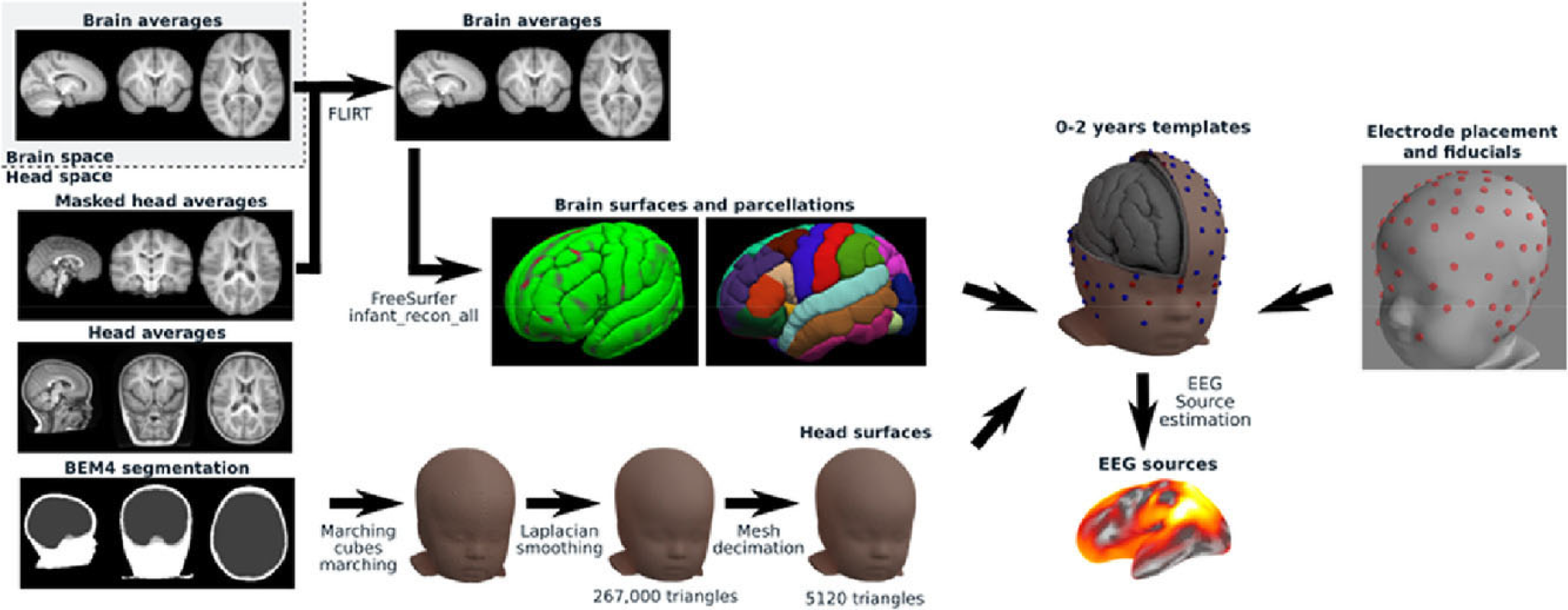
Head modeling pipeline [51]. Under a Creative Commons Licence (CC-BY-NC-ND) (https://creativecommons.org/licenses/by-nc-nd/4.0/). Permission granted by Elsevier.

Next, Xie et al. [50] (Figure 5) developed two SL pipelines and connectivity calculation for use in MATLAB, specifically designed for young children aged between 12 and 36 months. In particular, the first pipeline performs a phase-phase synchrony, while the second an amplitude-amplitude correlation. The steps in the pipeline are as follows; a) cortical source reconstruction of high-density EEG data using realistic MRI models with the utilization of age-appropriate MRI templates taken from the Neurodevelopmental MRI Database and the work by O’Reilly et al. [51], b) segmentation of anatomical MRI templates, c) creation of forward model via FEM and BEM for the first and second pipeline, respectively, d) inverse solution using eLORETA or minimum norm estimation, e) parcellation of reconstructed source areas into regions of interest, f) FC calculation.

Fig. 5

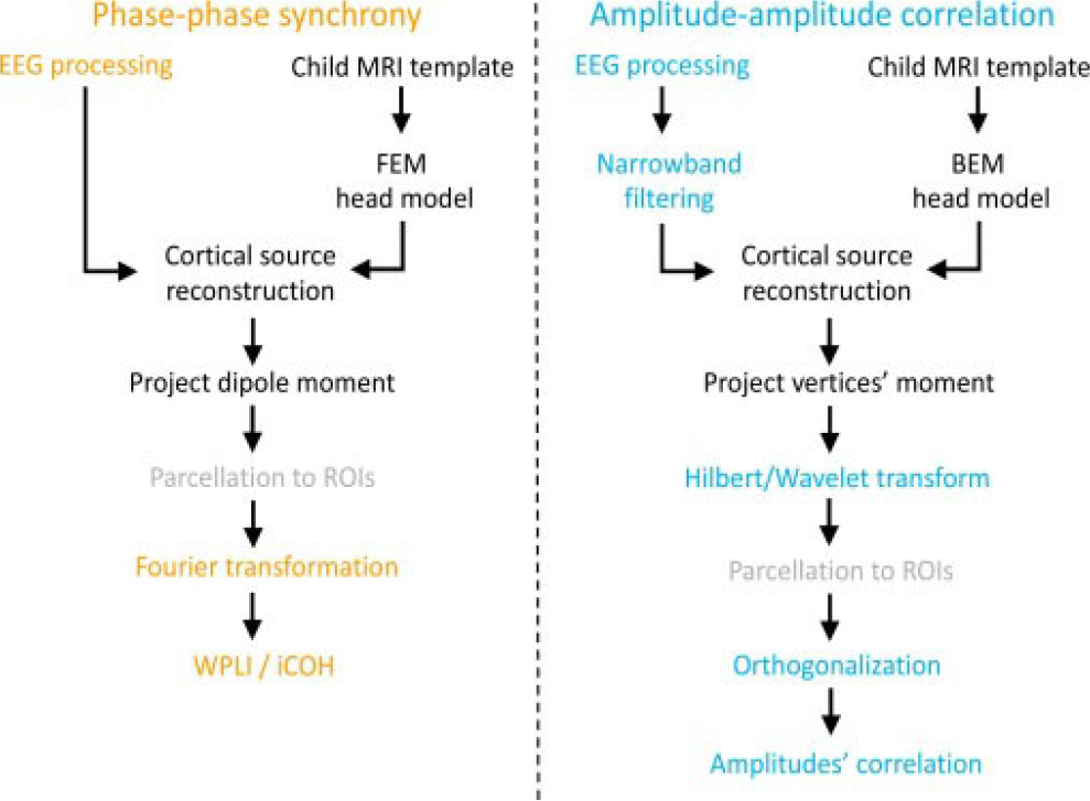
Source localization pipeline for two types (phase-phase synchrony and amplitude-amplitude correlation) of FC analysis [50]. Under Creative Commons Licence (CC BY) (https://creativecommons.org/licenses/by/4.0/) by Elsevier.

In addition to utilizing Fieldtrip and Brainstorm, the authors also employed the OpenMEEG toolbox to calculate the lead-field matrix for the second pipeline. Lastly, the authors applied age-appropriate conductivity values, orthogonalization, wPLI and the imaginary part of coherency.

Finally, several suggestions have been made to acquire better signal information for FC analysis and source localization. Firstly, high-density EEG recording is better for subsequent cortical source analysis [50, 51]. Secondly, as previously discussed, variations of coherency metrics have been proven better options for reducing volume conduction. For example, wPLI and orthogonalized power envelope correlation are considered “robust” linear (and probably non-linear for the former) FC metrics for the computation of phase-to-phase synchrony and amplitude-amplitude correlation respectively, with less influence by volume conduction [50]. Furthermore, various traditional machine learning (ML) algorithms are being more and more employed for infant-appropriate neural feature classification [209, 210] such as the support vector-machine [211] and random forests [212], usually for the identification of different cognitive states and disorders [213–216]. Notably, a recent ML tutorial proposed the combination of ML techniques with wPLI and Riemannian geometry for connectivity computation that is less affected by volume conduction and individual differences [209].

6 Discussion

It is well known that the FC analysis in the immature brain requires different type of data analysis compared to adults, as infants not only exhibit distinct brain characteristics (e.g. lower EEG band ranges, slow-wave domination, higher skull conductivity, different network anatomy, different head size etc), but also their initial EEG data often demonstrate increased motor artifacts, shorter lengths, increase influenced by volume conduction, therefore compromising data quality and analyzability. Thus, researchers often apply age-appropriate preprocessing and processing techniques.

However, there are still no universal recording, preprocessing and processing standards in the infantile population, resulting in different data quality due to the application of different techniques and thus making the final results challenging to compare.

Subsequently, over the last decade, various researchers have argued regarding the necessity of avoiding manual and/or non-pediatrically adapted automated procedures employed in adult studies and have attempted to develop age-appropriate tools (e.g. adjusted-ADJUST, infantile head models), techniques (e.g. different filtering, lower artifact thresholds, pre-and post-segmentation artifact correction) and pipelines (e.g. APICE) with the goal of ‘saving’ as much EEG data as possibly, while enhancing data quality and obtaining true FC measures.

Firstly, the three infantile preprocessing pipelines that were recently published for the EEGLAB, aimed to provide automated, age-appropriate and more flexible standards for preprocessing the infantile EEG data. Although, as a whole, they have been found to perform better than the manual and adult automated procedures, APICE follows the most intricate and more flexible process, especially during the artifact correction stage. In contrast, MADE applies the least complex artifact correction procedure.

In particular, one of MADE’s disadvantage is the use of high-pass filtering at 0.3 Hz before performing ICA, which compromises the effectiveness of the latter, as 1-2 Hz high-pass filtering is the general recommendation before ICA. However, MADE’s age-appropriate artifact thresholds, the use of the pediatric suitable tool for automated artifact correction/rejection (i.e. adjusted-ADJUST) and the providable option for post-segmentation artifact correction make it a better choice than most common preprocessing pipelines. Next, one of HAPPE’s disadvantage is the non-use of pediatric-suitable tool for the automated artifact correction phase (i.e. MARA). Nevertheless, its whole process is strengthened by the implementation of W-ICA and the option to adjust the analysis based on the number of the electrodes, allowing for a decrease of the number of electrodes to be analuzed. In fact, it has been argued that the less the number of the electrodes the higher the effectiveness of ICA. Interestingly, the same authors recently released a new pipeline (HAPPILEE) that is dedicated for the preprocessing of low-density EEG (i.e. 32 channels) which is frequently the case for the majority of the EEG studies that investigate FC. Lastly, APICE performs the most complex and flexible artifact correction procedure as this stage is repeated multiple times, using different algorithms with flexible adaptive thresholds based on the electrode, the individual and the EEG condition (i.e. resting or task state). Also, via its sub-pipelines, it allows for the avoidance of ICA and the 1–2 Hz high-pass filtering, thus ‘saving’ the slower oscillatory activity that infants exhibit in larger amounts than adults. In conclusion, APICE could be a better choice when the goal of the study is the investigation of slow oscillations, while providing the most options for preprocessing through its four different sub-pipelines. Nevertheless, it should be noted that APICE was tested in a limited amount of infants, in comparison with HAPPE which recruited higher numbers of individuals from three different health groups (i.e. typical, ASD and at-risk for ASD).

One of the main limitations of the three infantile preprocessing pipelines is that, due to their short ‘lifespan’, they have not been widely applied in studies. To the best of our knowledge only one FC study [57] used one of them (i.e. HAPPE). Additionally, none of them compared their artifact correction stage with AMICA, which is considered the most efficient ICA algorithm [217], with some infantile studies supporting its effectiveness [218].

It should also be mentioned that, in recent years, a few authors provided guidelines for preprocessing when performing FC analysis. In particular, they have suggested the use of automated preprocessing procedures, detrending methods instead of high-pass filtering, relative lengthy epoching (e.g. with 4 s being suggested by Miljevic et al. [18]) and AR. Nevertheless, these recommendations are based on adults studies and it is less clear whether infantile FC studies should also follow them or a variation of them.

Furthermore, the matter of electrode density is still under discussion, with some researchers supporting the appropriateness of high-density recording before coherence analysis with AR, and/or cortical source localization. In fact, it has been found that the network anatomy accuracy of graph theory analysis decreases with low-density EEG recording [18], something that is often the case in infant studies. On the other hand, it is suggested that high-density recording with short lengths compromises the effectiveness of ICA.

Therefore, although it is obvious that the researcher should always evaluate the pros and cons of low- and high-density recording based on the specific analysis goals, the latter may be the best option when the objective of the study is the calculation of FC, especially via graph theory analysis. In such instances, ICA should be avoided and preprocessing with APICE is recommended. In contrast, the extended recordings of sleeping participants may permit ICA more easily.

Regarding FC computation in infants, the (ordinary) coherence coefficient is a popular metric for signal synchrony and local/widespread FC with its results approaching those of fMRI [32, 116, 219, 220]. Nonetheless, one of the issues with performing coherence analysis is its susceptibility to volume conduction, with infants showing higher influence due to their unique anatomical features. This leads to an increased risk of computing false FC values and makes the task of source-localization even more difficult. Consequently, the researchers should often apply more rigorous techniques to overcome this problem.

Towards this goal, several connectivity metrics have been developed, such as the partial, imaginary, isolated effective and reduced coherencies and with CSD. Interestingly, the orthogonalized power envelope correlation and the wPLI are regarded as less influenced by volume conduction. In addition, FC studies often apply the FDR algorithm to decrease the chances of finding false-positive values.

Notably, in the last two decades, several pipelines have been developed for the calculation of age-appropriate source localization and head modeling. Among these pipelines, one specializes in the FC analysis that follows the localization of the EEG signals. However, it should be highlighted that the procedures recommended by Xie et al. [50] are specifically tailored for toddlers and may not be suitable for infants.

The limitation of linear connectivity analysis can be overcome by using non-linear metrics, which could be a more appropriate way to represent communication between the components of brain networks, especially when performing a longitudinal study in infants as their neural networks develop both linearly and non-linearly, based on the maturational stage and brain region. In particular, PPC, AAC and PAC have been associated with neural communication with the latter being the most frequently employed form of CFC. However, to the best of our knowledge, there has not been any specific recommendation regarding its utilization in infants, mostly due to its infrequent application in this population.

On the other hand, the use of graph theory analysis in infant studies is more common and offers a more detailed and visual understanding of both linear and non-linear FC. Some of the general observations that have been made, mostly by adult studies, suggest that the weighted graphs can provide thorougher information on network FC in comparison with the unweighted and undirected graphs, and proportional thresholding offers higher network stability but increases the risk of computing false connections. Also, even-though the ‘thresholding’ debate is ongoing, it has been argued that the most appropriate absolute thresholding, in both adults and infants, is between 0.1 and 0.5.

As displayed throughout the text, most of the studies we listed performed different recording, preprocessing and processing techniques in their small amount of data (their resting and active-states are approximately 2 and 2.5 min respectively), while the above preprocessing and processing recommendations were not followed with consistency. To begin, out of the thirty-five collected articles, twenty-nine conducted low-density recording. Secondly, aside from one study, none of the others opted to utilize the newly developed infantile preprocessing pipelines, although a significant portion of these studies took place prior to the publication of these pipelines. Thirdly, no study used piecewise detrending instead of high-pass filtering. Fourth, various studies that measured resting and active-state of the awake infantile brain used short epochs such as 3 s, 2 s and 1 s, while several others kept their data continuous. Fifth, even-though the majority of the studies chose pre-segmentation artifact correction procedure (with the exception of three studies), less flexible standards were often followed (e.g. set amplitude threshold for data rejection at 100 μV or even 50 μV instead of 150 μV). Notably, three studies performed both pre- and post-segmentation artifact correction procedure. Sixth, even-though most studies followed automated procedures, eight of them applied manual or semi-automated artifact correction processes, and while only a minority (with low-density recordings) performed ICA, two of them used low limit for high-pass filtering (i.e. 0.3 Hz), possibly compromising its effectiveness. Seventh, with the exception of five studies, AR was performed for re-referencing. Eighth, among the studies that employed graph theory analysis, only half of them conducted high-density EEG recording. Among these, three studies employed proportional thresholding, one employed absolute, one binary and the remaining three did not provide information on the used thresholding method. Also, half of them computed the weighted graph (directed or undirected) and the other half the adjacency or connectivity matrices. Ninth, source-localization analysis was performed by two graph theory analysis studies, via sLORETA and eLORETA. Tenth, various tools and techniques that allow the reduction of volume conduction effect were utilized by a few of the studies that performed coherence analysis and source localization; CSD coherence was calculated by two studies, orthogonalized power envelope correlation by one and isolated effective coherence by one. Eleventh, six overall studies applied FDR with different thresholds.

Thus, it becomes apparent that the studies often use different techniques and methods to analyze their data, potentially leading to data inconsistencies and making the comparison with each other more difficult.

Lastly, it is worth discussing that preprocessing of awake and sleeping states follows different steps. For instance, in the latter condition, researchers do not always perform artifact correction -and can even skip filtering- as they choose artifact-free segments in advance by visual inspection, as data length can last for a few hours. Also, if epoched, the segment-length is often longer than that of the awake state e.g. 30-seconds, 2-minutes or even 5-minutes. Nevertheless, automated artifact correction procedures are not rare in these types of studies, and short epochs (e.g. 1-second) can also be created if data length is less than 30 minutes.

In the end, more research is required to investigate the appropriateness of recording, preprocessing and processing techniques in infants at various maturational stages and clinical groups (e.g. premature, epileptic, ADHD), and during different recording states (i.e. sleeping, baseline, active state), with the goal of creating age-appropriate standards for EEG analysis and facilitating the easier comparability of the relative research. In addition, the usefulness of the newly made preprocessing and source-localization pipelines will eventually be shown as more studies apply them. We also propose the use of both linear and non-linear FC metrics for the study of the developing networks, to shed light on the dual nature of the developmental processes, while comparing these results with the more rigorous FC methods that were mentioned earlier.