Sage Journals: Discover world-class research

Abstract

From August 19 to 21, 2022, the BCI Controlled Robot Contest finals in the World Robot Contest 2022 were held in Beijing, China. Fifteen teams participated in the finals in the Algorithm Contest of Motor Imagery BCI. This paper introduces the algorithms in the motor imagery (MI) classification area, describes the competition content and set, and summarizes the algorithms and results of the top five teams in the finals.

First, the MI paradigm and the overview of the existing motor imagery brain–computer interface classification algorithms are introduced, followed by the introduction of the algorithms of the top five teams in the final step by step, including electroencephalography channel selection, data length selection, data preprocessing, data augmentation, classification network, training, and testing settings. Finally, the highlights and results of each algorithm are discussed.

Keywords

brain–computer interface motor imagery convolutional neural network EEGNet World Robot Contest 2022

1 Introduction

For many people with severe motor disabilities, the inability to communicate normally with the outside world can have a significant impact on their quality of life. In such cases, brain– computer interface (BCI) technology serves as a communication bridge that translates the neuronal activity of the human brain and communicates with outside devices through commands. BCI systems can be divided into many categories based on the neuroimaging technique used to capture neural activity. Based on neuroimaging techniques, noninvasive BCI systems can be divided into many categories, such as electroen-cephalography (EEG), magnetoencephalography, functional magnetic resonance imaging, and functional near infrared. Among these neuroimaging techniques, EEG is widely used due to its ease of use, safety, portability, relatively low cost, and most importantly, high temporal resolution [1].

EEG records the electrical fields produced by the active brain, which can be decoded to understand the physical and psychological status [2]. Motor imagery (MI) is one of the most widely used cognitive tasks based on sensorimotor rhythms (SMRs). EEG-based MI tasks are achieved by imagining a specific kinesthetic movement of an individual’s limbs without actually performing it [3]. The widely studied MI tasks include left hand, right hand, left foot, right foot, both feet, and tongue [4, 5]. They are also applied to other parts of the body, such as elbow extension/flexion [6] and finger movements [7].

EEG-based MI signals are widely used in healthcare [8] (such as controlling wheelchairs or robots [9, 10] and stroke rehabilitation [11]) to restore, recover, and even replace lost or impaired human body functions. In nonmedical applications, EEG-based MI signals are used for human enhancement, controlling driverless vehicles, gaming, and security domain identification and authentication [12 –15].

The working principle of the EEG-based MI-BCIs is the changes in SMRs. Based on neurophysiological research in the sensorimotor cortex, MI alters the mu (8–12 Hz) and beta (18–26 Hz) rhythms [16]. The energy modulation of brain rhythms due to an event in a specific frequency range is called event-related desynchronization (ERD)/event-related synchronization (ERS) [17]. Contralateral sensorimotor cortical EEG signals showed a decrease in the mu and beta bands, called ERD, representing a decrease in the amplitude of the activated cortical EEG signals. At the same time, the increased amplitude of the mu and beta bands in the resting state of the ipsilateral cortical signal is called ERS [18]. Since ERD/ERS is mixed with other brain activities, such as muscle movements and eye blinks, which are unintentionally generated by the users, the motor imagery brain–computer interface (MI-BCI) algorithm must distinguish MI activities from other involuntary actions in the control signal. The existing studies on MI-BCI include enhancing the recognition and classification performance of MI tasks, reducing calibration time, BCI illiteracy, asynchronous MI systems, increasing the number of commands, adaptive MI-BCI, online MI-BCI, and training protocol, among others [1, 19]. Focusing on online MI-BCI, this paper briefly introduces the existing MI-BCI approaches and details the top five approaches in the finals in the Algorithm Contest of Motor Imagery BCI in the World Robot Contest 2022.

The remainder of this paper is organized as follows. Section 2 introduces some existing MI-BCI approaches. Section 3 describes the competition content and set. Section 4 presents the algorithms and results of the top five teams in the finals. Section 5 summarizes the highlights of each team’s algorithm. Finally, Section 6 draws conclusions.

2 Overview of existing MI-BCI approaches

The framework of EEG-based MI-BCI generally includes data acquisition, preprocessing, feature extraction, and classification and evaluation. This section briefly introduces the existing approaches for preprocessing, feature extraction, and classification of MI signals.

To extract valuable MI components from the EEG signal, preprocessing includes four main parts: channel selection, signal filtering, signal normalization, and artifact removal.

In an existing research, more EEG channel signals are usually used to obtain more spatial information to improve performance. However, there may be channels that contain irrelevant or redundant information about the MI task. Therefore, using more EEG channels does not guarantee performance improvement [20]. Many studies related to channel selection are conducted to remove redundant channels irrelevant to the MI task [21 –25].

Based on the ERD/ERS of SMRs, signal filtering selects the most valuable frequency range for the MI tasks [26, 27].

Signal normalization refers to the uniform normalization of all channels on the time axis, with relative relationships still existing between different channels.

Artifact removal removes artifact noise and improves the signal-to-noise ratio.

MI recognition and classification are required after preprocessing. MI classification algorithms are categorized into two groups: traditional machine learning and deep learning (DL).

Traditional MI classification algorithms mainly extract domain (time domain, frequency domain, time-frequency domain, spatial domain, spatio-temporal domain) features and then utilize classifiers (linear discriminant analysis, support vector machine, shallow neural networks) to perform the classification task. Time-domain features, such as mean, variance, Hjorth parameters, and skewness, are extracted in the time domain at different time points or different periods [28]. The most popular frequency domain features and time-frequency features include fast Fourier transform (FFT) [29], short-time Fourier transform (STFT) [30], and wavelet transform (WT) [31]. Considered practical features, spatial domain features are most widely applied in MI classification tasks and designed to identify features from specific electrode locations on the scalp. Common spatial patterns (CSP) [32] and its derivatives [33 –38] are the most common feature extraction approaches for EEG-based MI signals. The spatio-temporal features include both temporal and spatial (channel) domain information. The primary spatio-temporal approach is based on the Riemannian manifold [39].

Common spatial patterns [32] aims to design spatial filters to maximize the difference in variance values between the two EEG spatio-temporal signal matrixes after filtering, thus obtaining feature vectors with a high degree of discrimination. The features are then fed into the classifier for classification. Covariance matrix diagonalization is the basic principle of CSP. For multi-classification tasks, CSP can construct multiple spatial filters using the One-Versus-One or One-Versus-Rest strategies. Sparse CSP [33], L1-norm-based CSP [34], stationary CSP [35], divergence CSP [36], and probabilistic CSP [37] enhance CSP [32] functionality by regularization or other techniques. Filter bank CSP (FBCSP) [38] is an extended version of CSP [32]. It first slices the data frequency band and performs CSP filtering on each sub-band after slicing.

When EEG data are acquired and converted into a sample covariance matrix (SCM), a Riemannian manifold is generated, which is different from the Euclidean space. Barachant et al. [39] introduced the mapped covariance matrix on the tangent space of Riemannian manifolds and the minimum distance to Riemannian mean in Riemann manifolds. Xie et al. [40] considered a particular case of the symmetric positive definite to derive a simple and effective bilinear sub-manifold learning algorithm, alleviating the overfitting and computational problems of traditional classification methods on high-level manifolds. There are also some recently proposed advanced algorithms related to Riemannian geometry or Riemannian manifold [41 –46] in MI-BCI.

Based on input formulation, DL for EEG-based MI classification can be divided into three categories [38]: features, topological maps, and raw signal values.

Features are extracted from the original signal and fed into a DL network for classification. Luo et al. [47] extracted spatial frequency sequential time slices from EEG signals using FBCSP and classified them using long short-term memory and gated recursive unit models.

The EEG signal is represented as a two- or three-dimensional image depending on the spatial topology of the electrodes [48].

Raw signal input utilizes the amplitude in the time domain and trains the neural network end to end. The average classification accuracy of algorithms based on raw signal input is higher than others [49], with no risk of information loss.

A convolutional neural network (CNN) is more widely employed among the different DL network frameworks [50]. EEGNet [51] is a parameter-light CNN architecture suitable for different EEG classification tasks, achieving remarkable performance in MI classification tasks. Shallow ConvNet [52], a CNN model specifically for oscillatory signals, is widely used in MI classification tasks. MI-EEGNET [53], a ConvNet based on Inception and Xception architectures, is proposed for MI classification. EEG-TCNet [54], improving EEGNet [51] by adding a temporal convolutional network (TCNet), shows better results in MI classification tasks. C2CM [55] is a novel CNN architecture with a new temporal data representation. Some recent multi-view, multi-scale, or multi-branch contributions [27, 56 –60] exhibited advanced performance levels. Adding feature fusion to CNN networks [60, 61] also demonstrated excellent results. Additionally, some applications of attention-based DL networks in MI have been developed in recent years. Song et al. [62] proposed EEG Conformer, a convolutional transformer for EEG decoding and visualization. Liu et al. [63] proposed TCACNet, a temporal and channel attention convolutional network for MI-EEG classification. Altaheri et al. [64] proposed an attention-based temporal convolutional network (ATCNet) for EEG-based MI classification.

The DL model capacity is adequate for MI classification; however, the small amount of MI data tends to result in network overfitting. Five popular approaches, which include data augmentation, dropout, batch normalization, transfer learning, and feature fusion, can be used to improve model performance [49]. Data augmentation expands the amount of data, thus solving the problem of MI data scarcity. Popular data augmentation approaches in MI classification include copying [52], sliding window overlap, spatially rotating [65], and adding perturbations. Dropout prevents overfitting by randomly removing some connections between neurons [51]. Batch normalization can speed up model learning, simplify the tuning process, stabilize network learning, and has a specific regularization effect. Transfer learning can be used to reduce the discrepancy in the data distribution between the training data (source domain) and testing data (target domain) and simultaneously solve the problems of individual differences and inadequate labeled training data [66]. In the case of small training data, transfer learning can capture knowledge from a pretrained network to help train the model better [67], reducing the training cost and the possibility of overfitting. In addition, transfer learning facilitates the transfer of knowledge from one subject to another and from one session to another [67], alleviating the problem of significant individual differences in EEG signals. Feature fusion improves model performance by combining various extracted features [60], which can combine information from different layers or models or fuse in-depth features with manually extracted features.

3 Experimental setup

3.1 Paradigm

The competition consists of three stages: stages A and B of the preliminaries and the finals.

Figure 1 shows the MI dataset composition in the finals. This dataset consists of EEG data from six subjects with three different MI tasks, namely, the imagination of movement of the left hand (class 1), right hand (class 2), and feet (class 3). Two sessions on different days were recorded for each subject, i.e., one for training and another for testing. Each session is comprised of six blocks separated by breaks. One block consists of 30 trials (10 for each class in a random order), yielding 180 per session.

Fig. 1

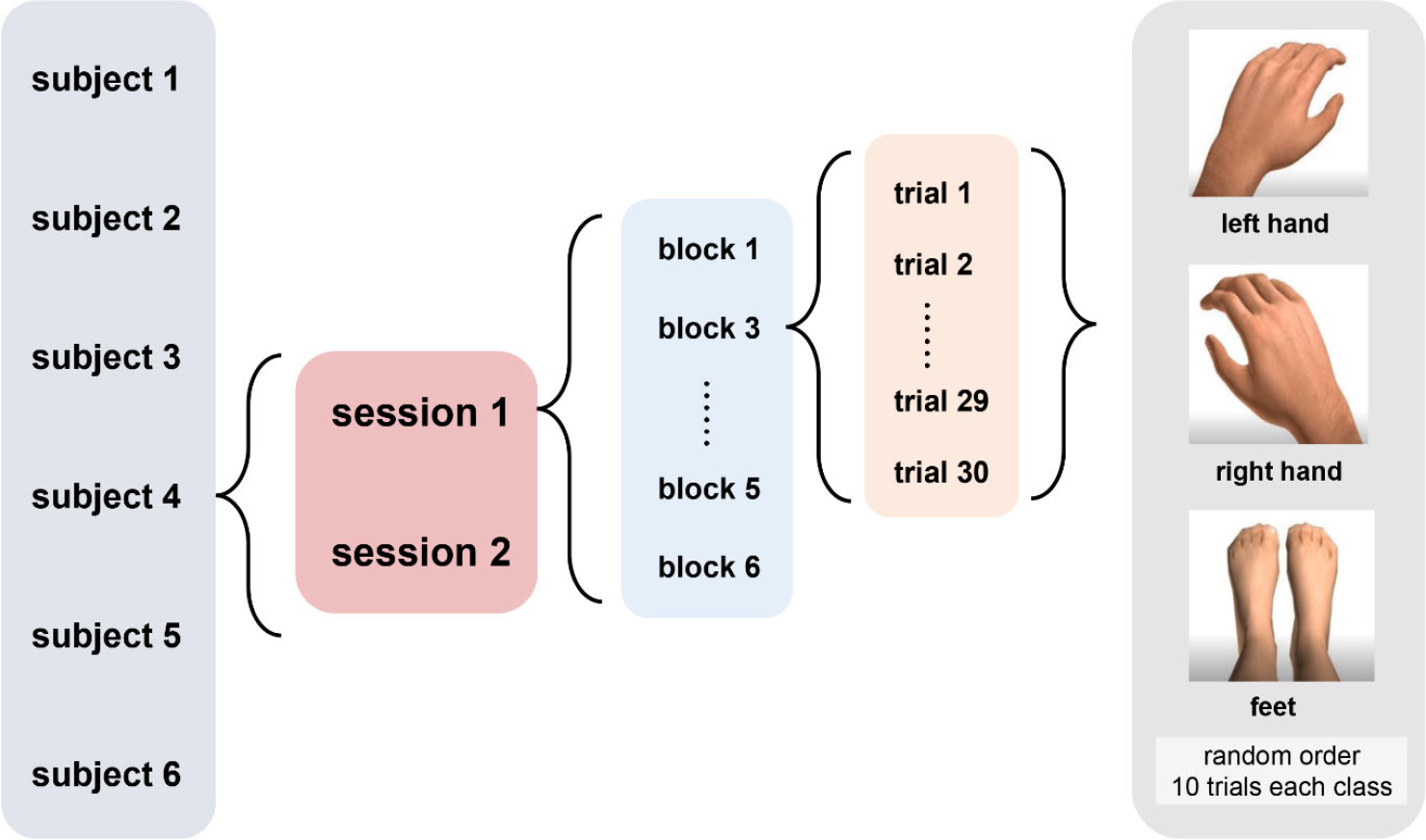
MI data composition in the finals.

In the experiment, the subjects sat in a comfortable armchair in front of a computer screen. At the beginning of a trial (t = 0), a cue in the form of a dynamic photo appeared and stayed on the screen for 2 s, prompting the subjects to perform the current MI task. The subjects were asked to perform the MI task for 5 s until the task photo disappeared from the screen at t = 7 s. After a short break, the subsequent trial (t = 12 s) was performed. Figure 2 shows the experimental procedure flowchart.

Fig. 2

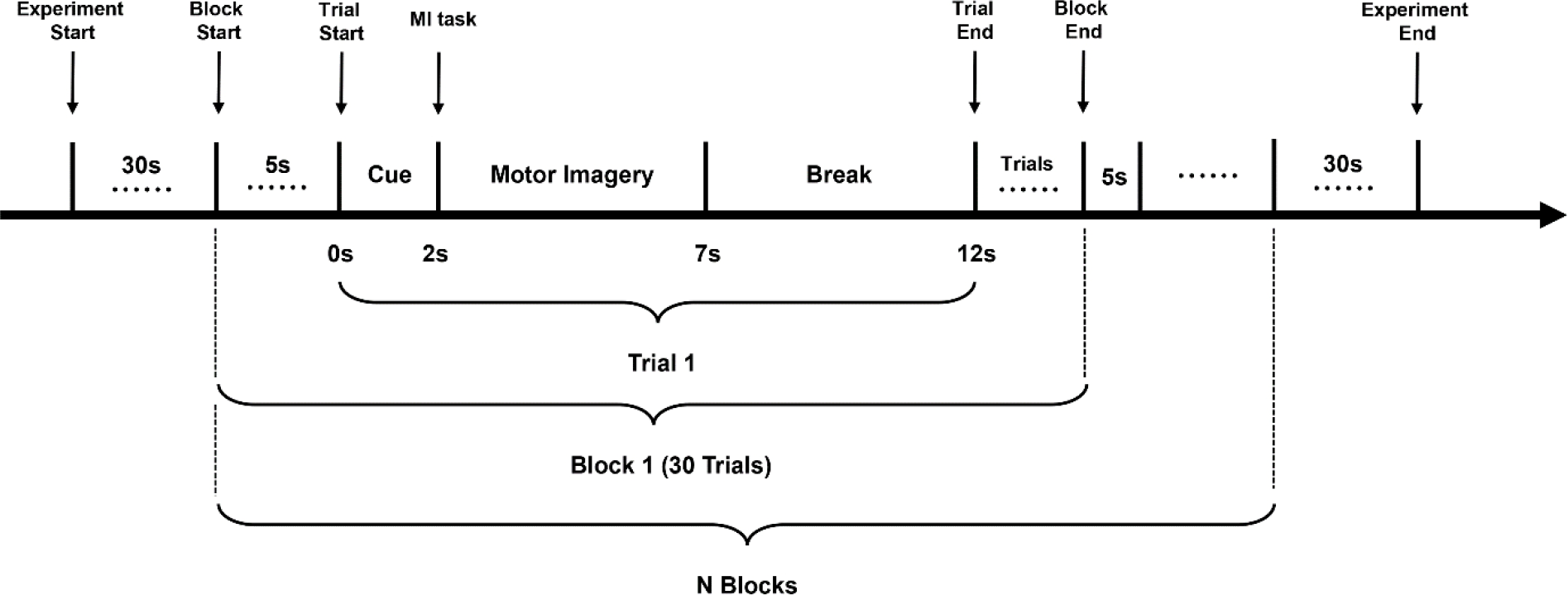
Experimental procedure flowchart.

A 64-channel acquisition device produced by Neuracle was used to acquire experimental data. The 65th lead was trigger information. The actual sampling rate was 1000 Hz, and the data were downsampled to 250 Hz. No other filtering was performed. The dataset paradigm provided by stages A and B were the same as the finals, except that stages A and B contained five subjects, respectively, and participants were provided with three blocks of data for each subject as training data and two blocks as test data.

3.2 Online test

In the preliminary stages A and B, participants were provided with three blocks of data for each subject as training data and two blocks as test data. Participants were required to train their models and upload them online for evaluation. In the finals, the test data were acquired at the competition site. The algorithm of each team was evaluated in real time, and the results were displayed on a large screen.

The dataflow is provided in a simulated online mode. The algorithm obtains a new data packet for each call to the datalog function, containing 40 ms of experimental EEG data and the trigger information. In the same block, packets are sent sequentially in time order. When the datalog function is called once, the competition system returns a new packet, which can be cached or processed. When the algorithm determines that the received data is sufficient to satisfy the judgment condition, it needs to call the feedback function to report the recognition results to the competition system. The competition system combines the effective data length with feedback accuracy to calculate the information translate rate (ITR).

3.3 Metric

The MI competition adopted the ITR as the evaluation criterion:

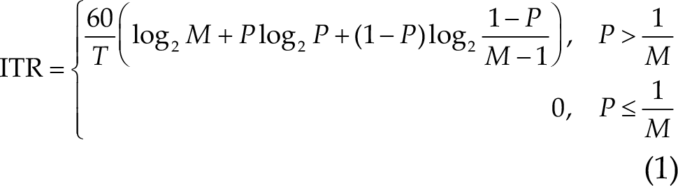
ITR = {\begin{array}{r} \frac{60}{T} (\log_{2} M + P \log_{2} P + (1 - P) \log_{2} \frac{1 - P}{M - 1}), & P > \frac{1}{M} \\ 0, & P \leq \frac{1}{M} \end{array}

where T denotes the average sampling time, M denotes the number of classes, and P denotes the recognition accuracy. The unit of ITR is bits/min. In particular, when the accuracy P is less than $\frac{1}{M}$ , i.e., the algorithm accuracy is less than random classification accuracy, the ITR is forced to be 0. When the system calculates the ITR, the average trial time includes a simulated rest time of 0.5 s.

The MI contest is designed as a triple classification task (M = 3). Figure 3 shows the relationship between the ITR and accuracy for average sampling time T. When T is fixed, it is observed that the higher the accuracy, the higher the ITR grows exponentially and nonlinearly. Assuming that T is 0.5 s, the average decision length is 125 time points when the sampling frequency is 250 Hz. When the accuracy is 0.6, 0.7, and 0.8, the ITR is 25.68, 48.44, and 79.56, respectively. When the classification accuracy is consistent, the ITR increases doubly with time by half. Assuming that the classification accuracies are 75%, the ITR is 62.84 and 31.42 when T = 0.5 s and T = 1 s, respectively. Therefore, the algorithms are required to improve efficiency by reducing the sampling time while ensuring as much accuracy as possible.

Fig. 3

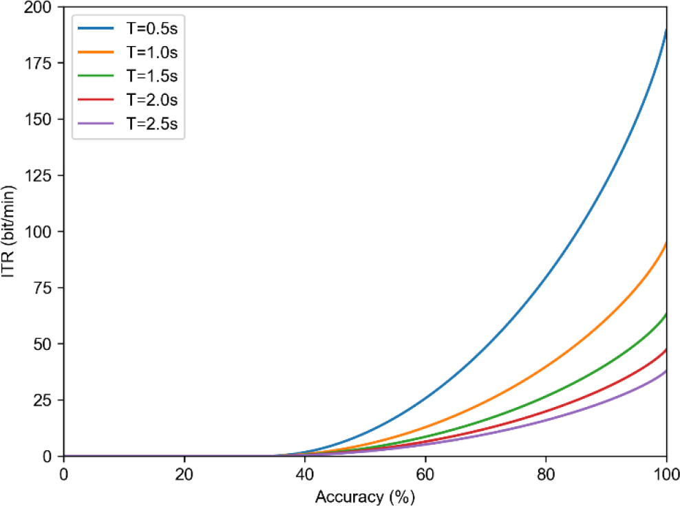
Relationship between the ITR and accuracy for average decision time T.

4 Methodology

4.1 EEG channel selection

Compared with other paradigms, MI does not require external stimulus signals. The subjects imagine the movements of the limbs or different parts of the body to induce changes in the activity of the relevant areas of the cerebral cortex. EEG signals with more channels are usually used to improve classification accuracy; however, there may be channels that contain irrelevant or redundant information related to MI tasks, which will affect the performance improvement of BCI. Therefore, selecting channels related to MI is beneficial to prevent noise signal interference and improve accuracy.

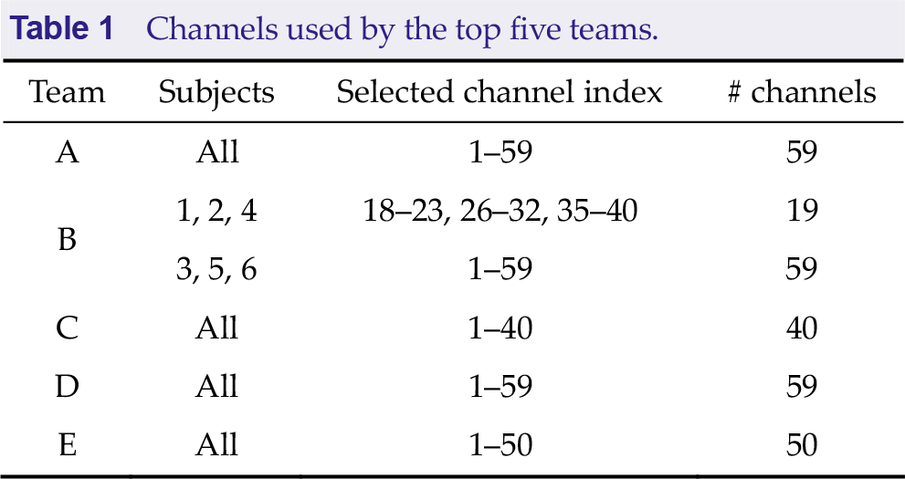
The contest provides 64 electrode signals, of which 1–59 are EEG channels. Figure 4 shows the EEG electrode index and name. Table 1 summarizes the EEG channels used by the top five teams. It is concluded that two teams selected all EEG channels, two manually selected specific EEG channels, and team B employed different channel selections for different subjects.

Fig. 4

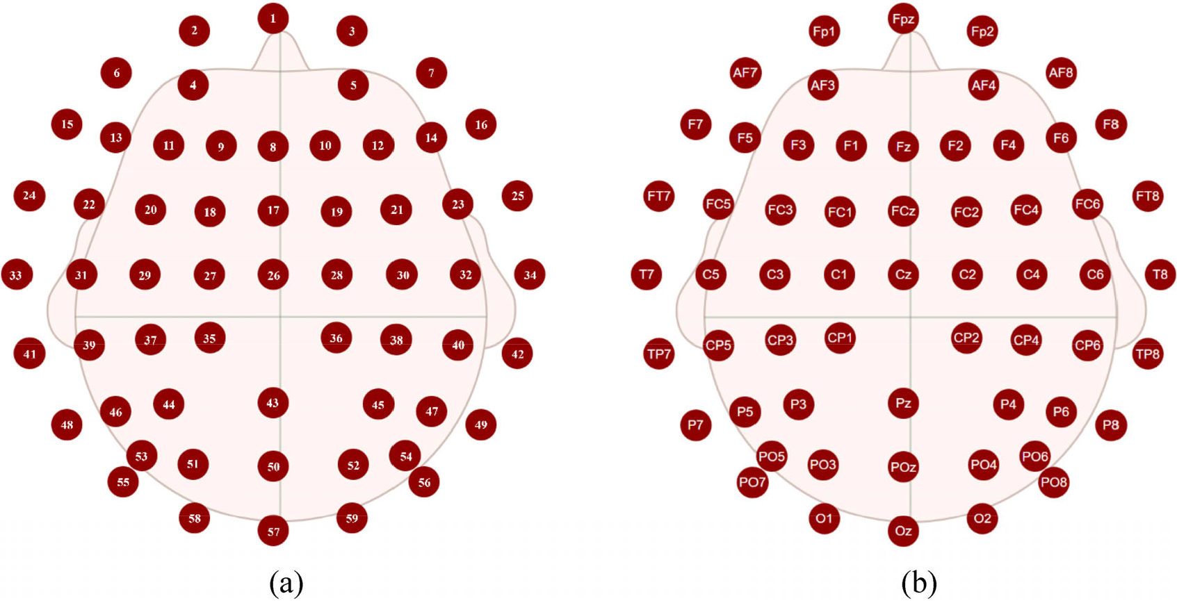
EEG electrode index and corresponding electrode name. (a) Electrode index. (b) Electrode name. Pictures from the Neuracle NeuSen W Series Wireless EEG Acquisition System.

Table 1

Channels used by the top five teams.

Team	Subjects	Selected channel index	# channels
A	All	1–59	59
B	1, 2, 4	18–23, 26–32, 35–40	19
B	3, 5, 6	1–59	59
C	All	1–40	40
D	All	1–59	59
E	All	1–50	50

4.2 Data length selection

The previous section introduced the metric ITR of the contest. Based on Eq. (1), both classification accuracy P and sampling time T affect the ITR.

Note that the two variables are nonlinearly related. ITR changes slowly near zero when the classification accuracy is close to the accuracy of random prediction, while it changes rapidly as the classification accuracy increases. Similarly, minimizing the sampling time with higher accuracy will result in more ITR improvement. However, shorter sampling times are typically associated with decreased accuracy. Therefore, better trading off the classification accuracy and sampling time for higher ITR is expected.

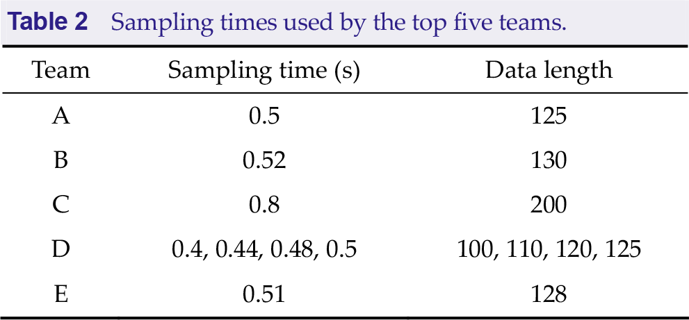
Table 2 summarizes the sampling time used by the top five teams. As the sampling rate is 250 Hz, the sampling points are calculated as data length. It was discovered that teams A, B, and E selected sampling times around 0.5 s, team D selected four different sampling times from 0.4 s to 0.5 s for training, and team C selected 0.8 s. The MI in the contest is a three-category classification task, and the test accuracy for most subjects is between 50% and 70%. In this range, the negative impact of increased accuracy is less significant than the negative impact of increased sampling time. Therefore, participants tend to lose test accuracy to gain higher ITR. In addition, all teams select a certain data length at the start of the trials.

Table 2

Sampling times used by the top five teams.

Team	Sampling time (s)	Data length
A	0.5	125
B	0.52	130
C	0.8	200
D	0.4, 0.44, 0.48, 0.5	100, 110, 120, 125
E	0.51	128

4.3 Data preprocessing

EEG signals have weak amplitudes and low signal-to-noise ratios due to irrelated components. Data preprocessing is a vital step to better extract helpful information.

The signal has some internal connection, which cannot be found clearly due to external noise. Detrending helps to eliminate the trend changes and presents the characteristics of the signal. Notch filter filters out signals in a specific frequency range, generally used to remove power interference signals. The bandpass filter removes frequency components irrelevant to the desired MI signal and retains the frequency range relevant to the MI signal.

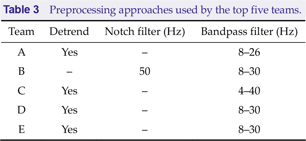
Table 3 summarizes the preprocessing approaches used by the top five teams. It should be noted that all teams chose Butterworth filters as bandpass filters. Team C chose third-order Butterworth filters, while the other teams chose fifth-order Butterworth filters. Team C first trained cross-subject models and then fine-tuned the models on the current subject. The input signals of all models were preprocessed in the same way.

Table 3

Preprocessing approaches used by the top five teams.

Team	Detrend	Notch filter (Hz)	Bandpass filter (Hz)
A	Yes	–	8–26
B	–	50	8–30
C	Yes	–	4–40
D	Yes	–	8–30
E	Yes	–	8–30

4.4 Data augmentation

The contest only provides 180 trials for training, which may easily cause overfitting with DL approaches. One trial contains 5 s data, while participants only use part of it. Data augmentation is essential to solve the problem of overfitting by using a more comprehensive set of data.

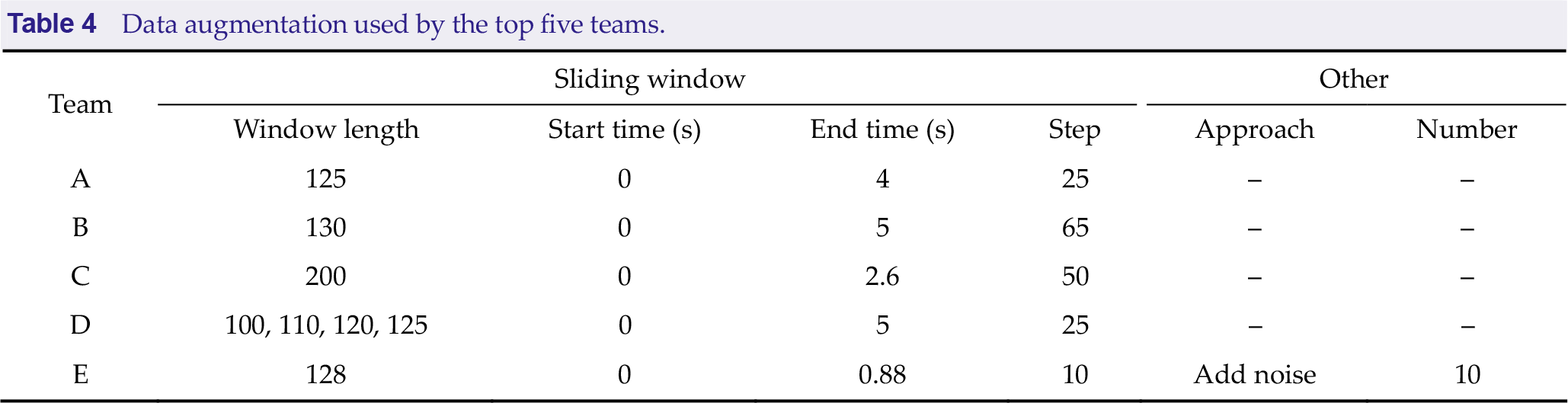
Table 4 summarizes the data augmentation used by the top five teams. All teams used sliding windows to enlarge the training set. The start time and end time represent the data segments in each trial of 5 s data for data augmentation. Step represents the number of sampling points between adjacent sliding windows. Team E applied sliding window augmentation before data preprocessing and then adds noise to the data, improving the robustness of the model:

noise = \frac{(λ \times σ^{2})}{2}

where λ is a randomly sampled parameter from a uniform distribution U(−0.5, 0.5) and σ ² is the variance of the data. Finally, they concatenated the noise-added data and the raw data.

Table 4

Data augmentation used by the top five teams.

Team	Sliding window				Other
Team	Window length	Start time (s)	End time (s)	Step	Approach	Number
A	125	0	4	25	–	–
B	130	0	5	65	–	–
C	200	0	2.6	50	–	–
D	100, 110, 120, 125	0	5	25	–	–
E	128	0	0.88	10	Add noise	10

4.5 Classification network

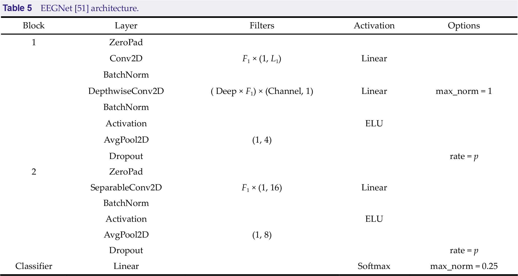
Deep learning has largely alleviated the requirement for manual feature extraction. In the past few years, deep CNNs have achieved excellent performance in EEG signal decoding. All teams in the contest used EEGNet for feature extraction and classification; however, slight differences in parameter settings were observed. Table 5 presents the EEGNet architecture. ZeroPad pads the input tensor boundaries with zero, and Conv2D indicates applying convolution over time dimension. DepthwiseConv2D indicates applying depth-wise convolutions to learn spatial filters within a temporal convolution. SeparableConv2D indicates applying separable convolutions to learn how to combine spatial filters across temporal bands optimally. BatchNorm, AvgPool2D, and ELU denote an operation of batch normalization, average pooling, and exponential linear unit activation function, respectively. Dropout indicates ignoring some neurons during the training process randomly. Maxnorm indicates regularizing each spatial filter by using a maximum norm constraint of 1 on its weights. Filters are represented as “kernel number” × (kernel size).

Table 5

EEGNet [51] architecture.

Block	Layer	Filters	Activation	Options
1	ZeroPad
	Conv2D	F1 × (1, L1)	Linear
	BatchNorm
	DepthwiseConv2D	(Deep × F ₁) × (Channel, 1)	Linear	max_norm = 1
	BatchNorm
	Activation		ELU
	AvgPool2D	1, 4)
	Dropout			rate = p
2	ZeroPad
	SeparableConv2D	F ₁ × (1, 16)	Linear
	BatchNorm
	Activation		ELU
	AvgPool2D	(1, 8)
	Dropout			rate = p
Classifier	Linear		Softmax	max_norm = 0.25

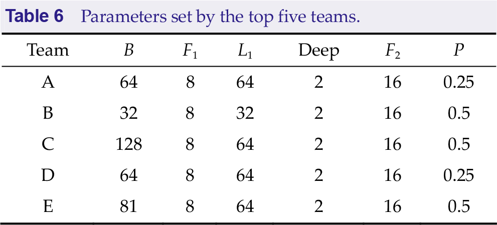
The input EEG signals were all organized in B × 1 × Channel × T, where B is the batch size, Channel is the number of channels (channel dimension), and T is the number of sampling points (time dimension). Table 6 summarizes the parameters set by the top five teams. F ₁ and F ₂ are the number of temporal and pointwise filters to learn, respectively, L ₁ is the length of temporal convolution in the first layer, deep is the number of spatial filters to learn within each temporal convolution, and p is the dropout rate.

Table 6

Parameters set by the top five teams.

Team	B	F ₁	L ₁	Deep	F ₂	P
A	64	8	64	2	16	0.25
B	32	8	32	2	16	0.5
C	128	8	64	2	16	0.5
D	64	8	64	2	16	0.25
E	81	8	64	2	16	0.5

4.6 Training and test settings

The approaches applied were introduced to prevent overfitting in the preprocessing stage. In the training stage, dividing the validation set and choosing an appropriate epoch can also prevent overfitting. Additionally, setting diverse seeds to train multiple models can stabilize the prediction output.

Table 7 summarizes the parameters set by the top five teams at the training stage. It was found that there were two forms to divide the validation set, randomly or by blocks. Random indicates randomly selecting part of the data as the validation set, and ratio is represented as “training set/validation set” in Table 7. Block denotes leaving the last or any block as the validation set. In the given maximum epochs, the models showing the best performance on the validation set are saved as the final models. The epoch selection method is represented as the “best epoch/maximum epoch” in Table 7.

Table 7

Parameters set by the top five teams at the training stage.

Team	Division		Epoch	Model number
Team	Setting	Ration	Epoch	Model number
A	Block	–	Best/100	11
B	–	–	50	1
C	Random	0.75/0.25	Best/1000	5
D	Block	–	Best/100	4*3
E	Random	0.9/0.1	Best/171	1

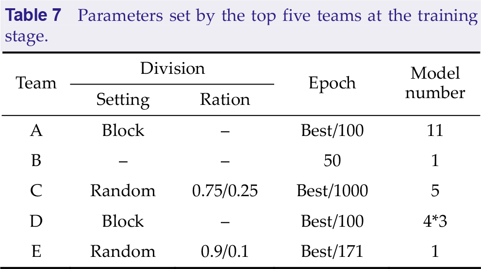
Team A selected the best epoch based on the validation set and then retrained all data according to the best epoch to obtain the final models. Team C first trained cross-subject models on data other than the target subjects and then fine-tuned the models with the target subject’s data. The validation division and epoch selection of these two phases were kept consistent and used five-fold cross-validation to obtain the final five models. The model number indicates the number of models trained for every subject. It should be noted that team D selected four different data lengths and trained three models at each data length.

Team C defined two training modes because of dividing the three trainings into two phases. For each phase of the training process for each subject, the mode that performs best on the validation set is selected for training.

Mode 1: All model weights can be updated and trained for 1000 epochs, of which the best performing model on the validation set is saved.

Mode 2: All model weights can be updated and trained for 1000 epochs. The third and fourth layer weights are frozen to train 200 epochs. The third and fourth are unfrozen and the first and second layers are frozen to train 200 epochs. The first and second layer weights are unfrozen to train 200 epochs. The best model in the last 200 epochs are selected to save.

All teams chose cross-entropy as the loss function, and Adam optimizer optimization update. Team B set the learning rate and weight decay to 0.01 and 0.001, respectively, while the other teams set the learning rate and weight decay to 0.001 and 0, respectively.

Data preprocessing and data length remained the same during the testing stage. For teams using multiple models for ensemble, they averaged all prediction probabilities and selected the category with the highest confidence as the final result. It should be noted that team A dropped the units in the model at the testing stage to prevent overfitting.

5 Results

The Algorithm Contest of Motor Imagery BCI includes preliminary stages A and B and the finals. The preliminary stages A and B were held online in July and August 2022, and the final stage was held in Beijing, China, from 19 to 21 August 2022.

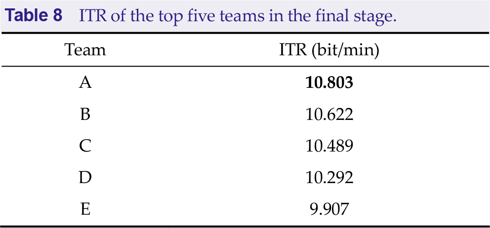
Table 8 presents the ITR of the top five teams in the final stage. Team A, from Huazhong University of Science and Technology, won the first place.

Table 8

ITR of the top five teams in the final stage.

Team	ITR (bit/min)
A	10.803
B	10.622
C	10.489
D	10.292
E	9.907

6 Summary

6.1 Team A

A suitable number of sliding window data augmentations were performed. It is presumed that the cerebral cortex is more active at the beginning of MI. Applying data augmentation for this part of the data can better expand the dataset and prevent overfitting. However, the end data contain only a little information or even have a negative impact.

Additionally, using a model ensemble for the prediction can make the output more stable.

6.2 Team B

Selecting different data channels for different subjects fuses knowledge and data to improve data quality, thus facilitating model training.

6.3 Team C

To cope with the problem of insufficient amount of MI data, Team C first trained the cross-subject model on data other than the target subjects and then fine-tuned it on the target subjects.

6.4 Team D

Team D also used a model ensemble for output prediction; however, each model was trained using a different length of data. Samples better distinguished at some lengths may have higher confidence at other lengths.

6.5 Team E

In addition to using sliding window augmentation, team E added noise to the current data and mixed it with the raw data for training to improve model robustness.

7 Conclusion

This paper reviewed the algorithms employed in the Algorithm Contest of Motor Imagery BCI in the BCI Controlled Robot Contest in WRC 2022. The participating algorithms varied based on traditional algorithms and DL end-to-end algorithms. However, the top five teams in the finals all utilized DL networks for feature extraction and classification, notably, with EEGNet as the backbone model. In recent years, DL has received increasing attention due to its good performance in MI classification. However, the generalizability and representativeness of the present DL networks for MI are not sufficient. It is expected that more generalizable and efficient DL networks will be implemented in MI classification tasks. In addition, data augmentation increases the robustness of the model. The top five teams in the finals all conducted data augmentation with sliding windows. The model ensemble facilitates the classification results more stable.

The overall test results of the final subjects were unsatisfactory, considering that the subjects may not have been trained in their imaginations or did not receive feedback when imagining. Therefore, it is difficult for algorithms to recognize the actual MI categories. The higher-ranked participating algorithms all use EEGNet as the backbone to train the classification model. Furthermore, the participating algorithms maintain a high degree of consistency in EEG length selection and data augmentation. In future research, it is expected that more diverse and innovative algorithms can be effectively employed in the competition. For MI tasks, the accuracy is more worthy of attention than the sampling time for prediction. The participating teams can consider how to improve the prediction efficiency of data far away from the decision surface without losing the accuracy.

Footnotes

Conflict of interests

All contributing authors report no conflict of interests in this work.

Funding

This research was supported by the STI 2030—Major Project (Grant No. 2021ZD0201300), Shenzhen Science and Technology Program (Grant No. JCYJ20220818103602004), Hubei Province Funds for Distinguished Young Scholars (Grant No. 2020CFA050).

Authors’ contribution

Jiayu An and Xinru Chen designed the study and analysed the results. All the authors were involved in writing the manuscript, and have approved the publishing version.

References

Singh

Hussain

Lal

, et al. A comprehensive review on critical issues and possible solutions of motor imagery based electroencephalography brain-computer interface. Sensors 2021, 21(6): 2173.

Binnie

Prior

. Electroencephalography. J Neurol Neurosurg Psychiatry 1994, 57(11): 1308–1319.

Lotze

Halsband

. Motor imagery. J Physiol Paris 2006, 99(4/5/6): 386–395.

Brunner

Leeb

Müller-Putz

, et al. BCI Competition 2008–Graz data set A. http://www.bbci.de/competition/iv

Leeb

Brunner

Muller-Putz

, et al. BCI Competition 2008{Graz data set B. https://www.researchgate.net/publication/238115253_BCI_Competition_2008_Graz_data_set_B

Grangeon

Guillot

Sancho

, et al. Rehabilitation of the elbow extension with motor imagery in a patient with quadriplegia after tendon transfer. Arch Phys Med Rehabil 2010, 91(7): 1143–1146.

Miao

Zeng

Wang

, et al. Index finger motor imagery EEG pattern recognition in BCI applications using dictionary cleaned sparse representation-based classification for healthy people. Rev Sci Instrum 2017, 88(9): 094305.

Rim

Sung

Min

, et al. Deep learning in physiological signal data: a survey. Sensors 2020, 20(4): 969.

Ron-Angevin

Velasco-Álvarez

Fernández-Rodríguez

, et al. Brain–computer interface application: auditory serial interface to control a two-class motor-imagery-based wheelchair. J Neuroeng Rehabil 2017, 14(1): 49.

10.

Fernández-Rodríguez

Velasco-Álvarez

Ron-Angevin

. Review of real brain-controlled wheelchairs. J Neural Eng 2016, 13(6): 061001.

11.

López-Larraz

Sarasola-Sanz

Irastorza-Landa

, et al. Brain–machine interfaces for rehabilitation in stroke: a review. NeuroRehabilitation 2018, 43(1): 77–97.

12.

van Erp

Lotte

Tangermann

. Brain–computer interfaces: beyond medical applications. Computer 2012, 45(4): 26–34.

13.

LaFleur

Cassady

Doud

, et al. Quadcopter control in three-dimensional space using a noninvasive motor imagery-based brain-computer interface. J Neural Eng 2013, 10(4): 046003.

14.

Zhou

Yin

, et al. Toward brain-actuated car applications: self-paced control with a motor imagery-based brain-computer interface. Comput Biol Med 2016, 77: 148–155.

15.

Zhang

Yao

Kanhere

, et al. MindID: Person identification from brain waves through attention-based recurrent neural network. Proc ACM Interact Mob Wearable Ubiquitous Technol 2018, 2(3): 1–23.

16.

Pfurtscheller

Brunner

Schlögl

, et al. Mu rhythm (de)synchronization and EEG single-trial classification of different motor imagery tasks. NeuroImage 2006, 31(1): 153–159.

17.

Neuper

Wörtz

Pfurtscheller

. ERD/ERS patterns reflecting sensorimotor activation and deactivation. Prog Brain Res 2006, 159: 211–222.

18.

Pfurtscheller

Neuper

. Future prospects of ERD/ERS in the context of brain-computer interface (BCI) developments. Prog Brain Res 2006, 159: 433–437.

19.

George

Smith

Madiraju

, et al. Motor imagery: a review of existing techniques, challenges and potentials. In 2021 IEEE 45th Annual Computers, Software, and Applications Conference (COMPSAC). Madrid, Spain, 2021, pp 1893–1899.

20.

Asensio-Cubero

Gan

Palaniappan

. Multiresolution analysis over simple graphs for brain computer interfaces. J Neural Eng 2013, 10(4): 046014.

21.

Feng

Jin

Daly

, et al. An optimized channel selection method based on multifrequency CSP-rank for motor imagery-based BCI system. Comput Intell Neurosci 2019, 2019: 8068357.

22.

Jin

Miao

Daly

, et al. Correlation-based channel selection and regularized feature optimization for MI-based BCI. Neural Netw 2019, 118: 262–270.

23.

Varsehi

Firoozabadi

SMP

. An EEG channel selection method for motor imagery based brain-computer interface and neurofeedback using Granger causality. Neural Netw 2021, 133: 193–206.

24.

Han

Zhao

Sun

, et al. A fast, open EEG classification framework based on feature compression and channel ranking. Front Neurosci 2018, 12: 217.

25.

Meng

Dong

Gao

, et al. Correlation and sparse representation based channel selection of motor imagery electroencephalogram (in Chinese). J Electron Inf Technol 2022, 44(2): 477–485.

26.

Shajil

Mohan

Srinivasan

, et al. Multiclass classification of spatially filtered motor imagery EEG signals using convolutional neural network for BCI based applications. J Med Biol Eng 2020, 40(5): 663–672.

27.

Jia

Lin

Wang

, et al. MMCNN: a multi-branch multi-scale convolutional neural network for motor imagery classification. In Machine Learning and Knowledge Discovery in Databases: European Conference, ECML PKDD 2020. Lecture Notes in Computer Science, vol 12459. Hutter Kersting

Lijffijt

Cham: Springer, 2021, pp 736–751.

28.

Pawar

Dhage

. Feature extraction methods for electroencephalography based brain-computer interface: a review. IAENG Int J Comput Sci 2020, 47(3): 501–515.

29.

Djamal

Abdullah

Renaldi

. Brain computer interface game controlling using fast Fourier transform and learning vector quantization. J Telecomm Electron Comput Eng (JETC) 2017, 9(2–5): 71–74.

30.

Wang

Cao

Zhang

, et al. Short time Fourier transformation and deep neural networks for motor imagery brain computer interface recognition. Concurrency Computat Pract Exper 2018, 30(23): e4413.

31.

Hsu

Sun

. EEG-based motor imagery analysis using weighted wavelet transform features. J Neurosci Methods 2009, 176(2): 310–318.

32.

Lotte

Guan

. Regularizing common spatial patterns to improve BCI designs: unified theory and new algorithms. IEEE Trans Biomed Eng 2011, 58(2): 355–362.

33.

Arvaneh

Guan

Ang

, et al. Optimizing the channel selection and classification accuracy in EEG-based BCI. IEEE Trans Biomed Eng 2011, 58(6): 1865–1873.

34.

Wang

Tang

Zheng

. L1-norm-based common spatial patterns. IEEE Trans Biomed Eng 2012, 59(3): 653–662.

35.

Samek

Vidaurre

Müller

, et al. Stationary common spatial patterns for brain–computer interfacing. J Neural Eng 2012, 9(2): 026013.

36.

Samek

Kawanabe

Müller

. Divergence-based framework for common spatial patterns algorithms. IEEE Rev Biomed Eng 2014, 7: 50–72.

37.

Chen

Gao

, et al. Probabilistic common spatial patterns for multichannel EEG analysis. IEEE Trans Pattern Anal Mach Intell 2015, 37(3): 639–653.

38.

Ang

Chin

Zhang

, et al. Filter bank common spatial pattern (FBCSP) in brain-computer interface. In 2008 IEEE International Joint Conference on Neural Networks (IEEE World Congress on Computational Intelligence) . Hong Kong, China, 2008, pp 2390–2397.

39.

Barachant

Bonnet

Congedo

, et al. Multiclass brain–computer interface classification by Riemannian geometry. IEEE Trans Biomed Eng 2012, 59(4): 920–928.

40.

Xie

, et al. Motor imagery classification based on bilinear sub-manifold learning of symmetric positive-definite matrices. IEEE T Neur Sys Reh 2017, 25(6): 504–516.

41.

Chu

Zhao

Zou

, et al. Decoding multiclass motor imagery EEG from the same upper limb by combining Riemannian geometry features and partial least squares regression. J Neural Eng 2020, 17(4): 046029.

42.

Larzabal

Auboiroux

Karakas

, et al. The Riemannian spatial pattern method: mapping and clustering movement imagery using Riemannian geometry. J Neural Eng 2021, 18(5): 056014.

43.

Jin

, et al. Motor imagery EEG classification based on Riemannian sparse optimization and dempster-shafer fusion of multi-time-frequency patterns. IEEE T Neur Sys Reh 2023, 31: 58–67.

44.

Singh

Lal

Guesgen

. Motor imagery classification based on subject to subject transfer in Riemannian manifold. In 2019 7th International Winter Conference on Brain-Computer Interface (BCI). Gangwon, Korea (South), 2019, pp 1–6.

45.

Mishra

Jagadish

Kiran

MPRS

, et al. A novel classification for EEG based four class motor imagery using kullback-leibler regularized Riemannian manifold. In 2018 IEEE 20th International Conference on e-Health Networking, Applications and Services (Healthcom). Ostrava, Czech Republic, 2018, pp 1–5.

46.

Guan

Zhao

Yang

. Motor imagery EEG classification based on decision tree framework and Riemannian geometry. Comput Intell Neurosci 2019, 2019: 5627156.

47.

Luo

Zhou

Chao

. Exploring spatial-frequency-sequential relationships for motor imagery classification with recurrent neural network. BMC Bioinformatics 2018, 19(1): 344.

48.

Liao

Luo

Yang

, et al. Effects of local and global spatial patterns in EEG motor-imagery classification using convolutional neural network. Brain Comput Interfaces 2020, 7(3/4): 47–56.

49.

Al-Saegh

Dawwd

Abdul-Jabbar

. Deep learning for motor imagery EEG-based classification: a review. Biomed Signal Process Contr 2021, 63: 102172.

50.

Altaheri

Muhammad

Alsulaiman

, et al. Deep learning techniques for classification of electroencephalogram (EEG) motor imagery (MI) signals: a review. Neural Comput Appl 2023, 35(20): 14681–14722.

51.

Lawhern

Solon

Waytowich

, et al. EEGNet: a compact convolutional neural network for EEG-based brain-computer interfaces. J Neural Eng 2018, 15(5): 056013.

52.

Schirrmeister

Springenberg

Fiederer

LDJ

, et al. Deep learning with convolutional neural networks for EEG decoding and visualization. Hum Brain Mapp 2017, 38(11): 5391–5420.

53.

Riyad

Khalil

Adib

. MI-EEGNET: a novel convolutional neural network for motor imagery classification. J Neurosci Methods 2021, 353: 109037.

54.

Ingolfsson

Hersche

Wang

, et al. EEG-TCNet: an accurate temporal convolutional network for embedded motor-imagery brain–machine interfaces. In 2020 IEEE International Conference on Systems, Man, and Cybernetics (SMC) . Toronto, ON, Canada, 2020, pp 2958–2965.

55.

Sakhavi

Guan

Yan

. Learning temporal information for brain-computer interface using convolutional neural networks. IEEE Trans Neural Netw Learn Syst 2018, 29(11): 5619–5629.

56.

Mane

Chew

Chua

, et al. FBCNet: a multi-view convolutional neural network for brain-computer interface. arXiv 2021, arXiv: 2104.01233. https://arxiv.org/abs/2104.01233

57.

Liu

Yang

, et al. FBMSNet: A filter-bank multi-scale convolutional neural network for EEG-based motor imagery decoding. IEEE T Bio-med Eng 2022, 70(2): 436–445.

58.

Niu

, et al. A parallel multiscale filter bank convolutional neural networks for motor imagery EEG classification. Front Neurosci 2019, 13: 1275.

59.

Zhao

Zhang

Zhu

, et al. A multi-branch 3D convolutional neural network for EEG-based motor imagery classification. IEEE T Neur Sys Reh 2019, 27(10): 2164–2177.

60.

Amin

Alsulaiman

Muhammad

, et al. Deep Learning for EEG motor imagery classification based on multi-layer CNNs feature fusion. Future Gener Comput Syst 2019, 101: 542–554.

61.

Musallam

AlFassam

Muhammad

, et al. Electroencephalography-based motor imagery classification using temporal convolutional network fusion. Biomed Signal Proces 2021, 69: 102826.

62.

Song

Zheng

Liu

, et al. EEG conformer: Convolutional transformer for EEG decoding and visualization. IEEE T Neur Sys Reh 2023, 31: 710–719.

63.

Liu

Shi

Hui

, et al. TCACNet: temporal and channel attention convolutional network for motor imagery classification of EEG-based BCI. Inform Process Manag 2022, 59(5): 103001.

64.

Altaheri

Muhammad

Alsulaiman

. Physics-informed attention temporal convolutional network for EEG-based motor imagery classification. IEEE T Ind Inform 2023, 19(2): 2249–2258.

65.

Krell

Kim

. Rotational data augmentation for electroencephalographic data. In 2017 39th Annual International Conference of the IEEE Engineering in Medicine and Biology Society (EMBC). Jeju, Korea (South), 2017, pp 471–474.

66.

Weiss

Khoshgoftaar

Wang

. A survey of transfer learning. J Big Data 2016, 3: 9.

67.

Zhu

, et al. Separated channel convolutional neural network to realize the training free motor imagery BCI systems. Biomed Signal Proces 2019, 49: 396–403.

Algorithm contest of motor imagery BCI in the World Robot Contest 2022: A survey

Abstract

Keywords

1 Introduction

2 Overview of existing MI-BCI approaches

3 Experimental setup

3.1 Paradigm

3.2 Online test

3.3 Metric

4 Methodology

4.1 EEG channel selection

4.2 Data length selection

4.3 Data preprocessing

4.4 Data augmentation

4.5 Classification network

4.6 Training and test settings

5 Results

6 Summary

6.1 Team A

6.2 Team B

6.3 Team C

6.4 Team D

6.5 Team E

7 Conclusion

Footnotes

Conflict of interests

Funding

Authors’ contribution

References