
Abstract
Recently, rapid serial visual presentation (RSVP), as a new event- related potential (ERP) paradigm, has become one of the most popular forms in electroencephalogram signal processing technologies. Several improvement approaches have been proposed to improve the performance of RSVP analysis. In brain–computer interface systems based on RSVP, the family of approaches that do not depend on training specific parameters is essential. The participating teams proposed several effective training-free frameworks of algorithms in the ERP competition of the BCI Controlled Robot Contest in World Robot Contest 2021. This paper discusses the effectiveness of various approaches in improving the performance of the system without requiring training and suggests how to apply these approaches in a practical system. First, appropriate preprocessing techniques will greatly improve the results. Then, the non-deep learning algorithm may be more stable than the deep learning approach. Furthermore, ensemble learning can make the model more stable and robust.
Keywords
1 Introduction
Brain–computer interface (BCI) provides people with an alternative way to communicate with external devices, which can directly measure the user’s brain activity and converts it into the corresponding signal in the BCI [1]. The electro- encephalogram (EEG) is the most commonly used input signal in BCIs because of its simplicity [2]. The measurement method of brain activity is used in functional near-infrared, functional magnetic resonance, and EEG [3]. Additionally, using EEG signals for affective interaction can make interfaces more intuitive [4].
P300 evoked potential [5], motor imagery [6], and rapid serial visual presentation (RSVP) [7] are widely used paradigms in BCIs. RSVP is one form in which visual stimuli are displayed rapidly (2–20 Hz) in chronological order at a fixed position on screen [8], and EEG recordings of subjects’ brain activities are collected throughout the experiment. Specifically, RSVP is an EEG signal induced by small probability events. After stimulation, RSVP will have a positive peak in EEG data. Additionally, RSVP is the response in the time domain.
Figure 1 shows the workflow of RSVP used in the event-related potential (ERP) competition (training-free) of the World Robot Contest 2021 (WRC2021), meaning that each subject has an independent classifier.
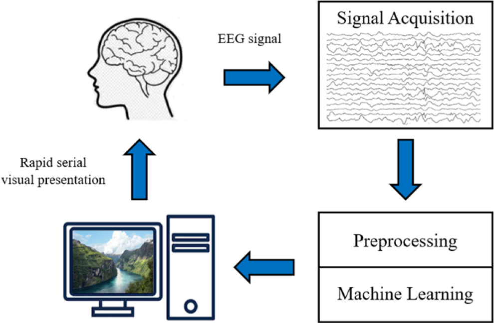
Workflow of RSVP.
First, the subjects are shown with specific images at a high presentation rate on the computer screens, and their brains generate associated RSVP signals. After feature extraction, the contestants use the algorithms to give the corresponding prediction results. Finally, the organizing committee judges the prediction accuracy.
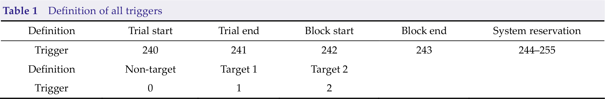
During each trial, subjects had a preparation time of 2000 ms at first and were then showed a new picture displayed on the screen every 100 ms. The images include target and non-target images. For this ERP competition, Table 1 presents the definition of the triggers; the target images are cars (label 1) and humans (label 2), whereas the non-target images are backgrounds (label 0). Additionally, a data imbalance problem exists: RSVP data contain many non-target images and only a small number of target images, with a ratio of around 15:1, which becomes a great challenge for algorithm designs.
Definition of all triggers
Many algorithms based on traditional machine learning have been proposed for single-trial RSVP EEG classification. Linear discriminant analysis (LDA) and Fisher LDA (FLD) have been widely used in these classical algorithms. For example, hierarchical discriminant component analysis (HDCA) and spatially weighted FLD principal component analysis (PCA; SWFP) are two popular classical algorithms.
Specifically, HDCA uses LDA to obtain spatial weighting vectors for different time periods to calculate the projections of the single-trial RSVP EEG data. SWFP algorithm learns a spatio- temporal weights matrix through FLD to amplify discriminative components and then uses PCA to reduce temporal dimension [9]. Most traditional methods are linear algorithms. However, linear constraint makes traditional methods train faster and more robust, limiting the classification performance [10].
Furthermore, many new convolutional neural network (CNN) models have been proposed for single-trail RSVP EEG classification, such as ShallowConvNet, DeepConvNet [11], which will be introduced in detail in the following sections. Shaheen et al. [12] proposed a deep belief net classifier to classify single-trial RSVP EEG data. Zang et al. [13] also proposed PLNet to classify single-EEG data. They obtained that the net is more efficient than most deep learning methods.
In this paper, we introduce the algorithms used by the top-five teams (Hust-BCI, pikapika, Brainstorming, XDU_ERP, Mind Reader) in the finals of the ERP competition (training-free) of the WRC2021. For simplicity, the algorithms of the five teams will be called Algo-H (Hust-BCI), Algo-P (pikapika), Algo-B (Brainstorming), Algo-X (XDU_ERP), and Algo-M (Mind Reader). The five teams will be called Team-H (Hust-BCI), Team-P (pikapika), Team-B (Brainstorming), Team-X (XDU_ERP), and Team-M (Mind Reader). This paper aims to evaluate the performance of different algorithms in the training-free scenario.
2 Methods
In this section, we first introduce preprocessing approaches, such as filter and Euclidean space alignment (EA) [14]. Then, we introduce two frameworks, because only Team-H uses the non-deep learning framework, while other teams use the deep learning framework. The non-deep learning framework mainly includes xDAWN [15], tangent space mapping [16], and logistic regression [17]. The deep learning frameworks apply networks such as EEGNet, DeepConvNet, and long short-term memory (LSTM) [18], which are usually used in BCI. Finally, we introduce the training strategy in a training-free scenario and flowcharts of the five teams.
2.1 Experimental arrangement
Figure 2 shows the detailed layout of RSVP. During each trial, subjects had a preparation time of 2000 ms at first and were then showed a new picture displayed on the screen every 100 ms. The images include target and non-target images, approved by the institutional review board of Tsinghua University (NO. 20210032).
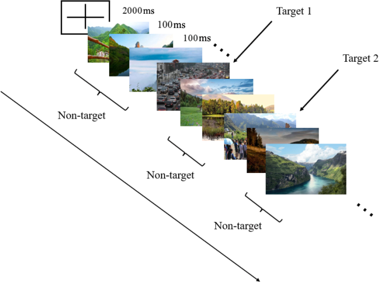
RSVP in BCI competition.
For this ERP competition, Table 1 presents the definition of the triggers; the target images are cars (label 1) and humans (label 2), whereas the non-target images are backgrounds (label 0). Additionally, a data imbalance problem exists: RSVP data contain many non-target images and only a small number of target images, with a ratio of around 15:1, which becomes a great challenge for algorithm designs. In the computational aspect, a successful BCI system must address the following two issues. First, a successful BCI system must extract the event-specific signatures that characterize the brain signals specific to the target (or non-target) images embedded in the EEG recordings. This is often enforced by a training process, where the signatures are extracted from the training data whose event associations are already known. Second, a successful BCI system must effectively utilize the event-specific signatures to classify EEG recordings whose event association is unknown. This is often enforced by a classifier in the testing process.
Figure 3 shows the data collection process of the competition. There were four subjects in the competition. For each subject, the organizing committee collects three blocks with 10 trials in each block.
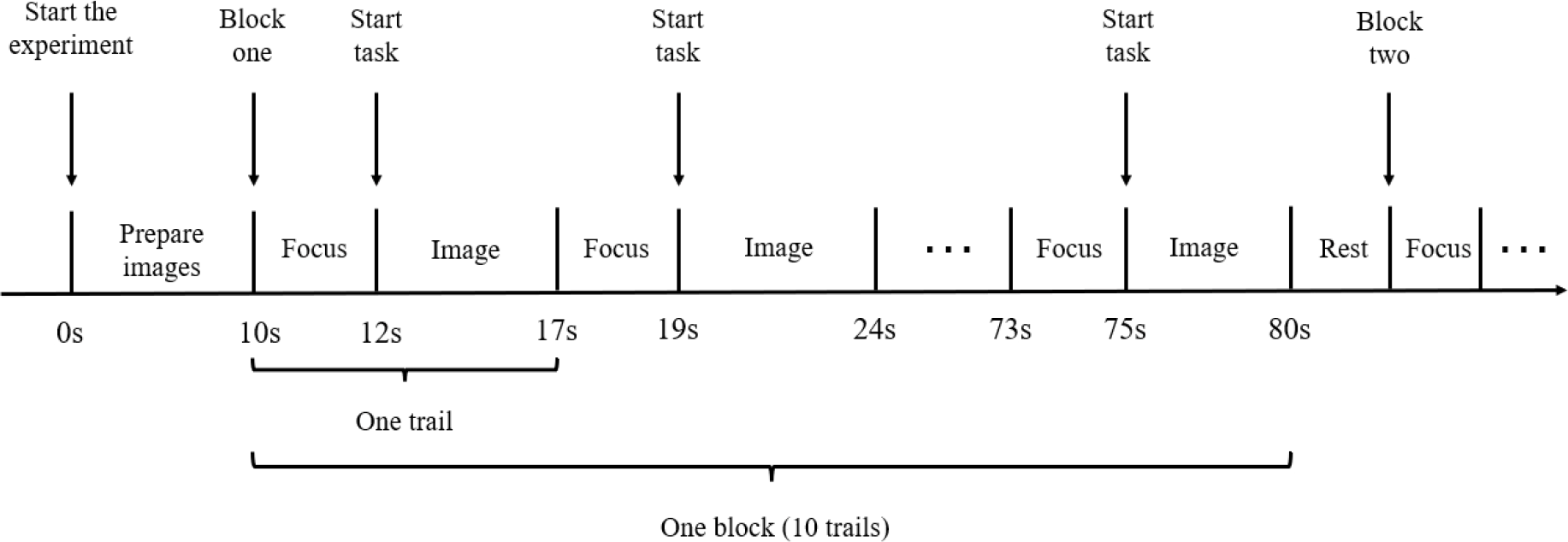
Data collection process of the competition.
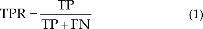
The following equation defines the competition’s evaluation metric, true positive rate (TPR). Here TP refers to the total number of the data with labels 1 and 2 that the model correctly predicts; FN refers to the total number of the data with labels 1 and 2 that the model wrongly predicts.
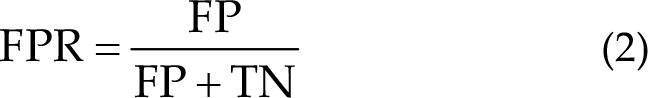
The following equation defines the evaluation metric, false positive rate (FPR). Here, FP refers to the total number of the data with label 0 that the model wrongly predicts; TN refers to the total number of the data with label 0 that the model correctly predicts.
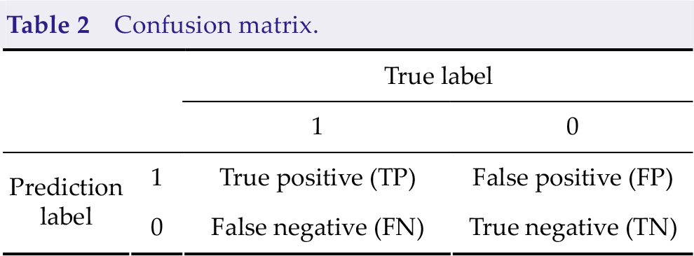
A more specific explanation is shown in Table 2. Receiver operating characteristic (ROC) and area under the curve (AUC) are often used to evaluate the advantages and disadvantages of a binary classifier. In Fig. 4, the ordinate of the ROC curve is TPR, and the abscissa of ROC is FPR.
Confusion matrix.
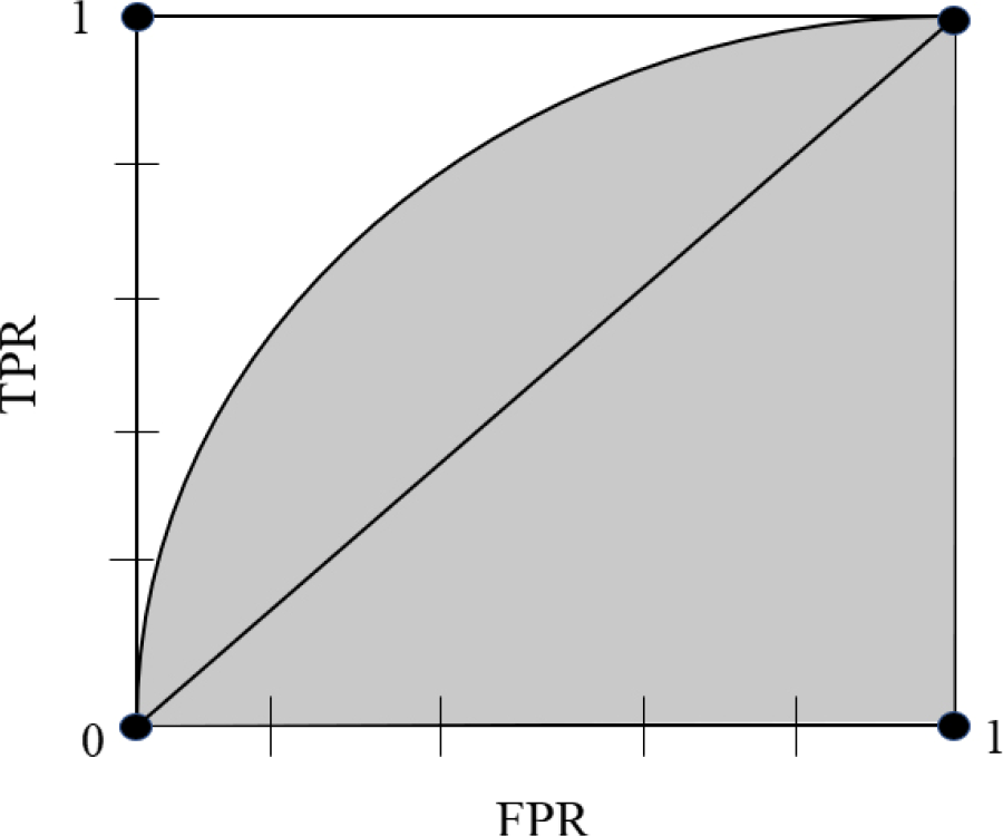
AUC and ROC.
AUC is one of the main offline evaluation indicators used by classification models, especially binary classification models. There are two meanings of AUC. One is the traditional meaning of “area under ROC curve”, and it is the shaded part in Fig. 4.
The other is about the explanation of sorting ability. For example, the meaning of AUC of 0.7 can be roughly understood as follows: given a positive sample and a negative sample, in 70% of cases, the model scores the positive sample higher than the negative sample. It can be seen that under this explanation, we are only concerned about the score between positive and negative samples, while the specific score is irrelevant. The equation is given as follows:

Here, PTrue is the probability of predicting the positive sample as 1; PFalse refers to the probability of predicting the negative sample as 1.
2.2 Preprocessing approach
2.2.1 Filter
Among the five teams in the competition, only Team-B did not use filters.
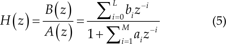
Team-H used infinite impulse response (IIR) filters to filter data along one dimension after training parameters based on previous training sets without a bandpass filter, where IIR filters follow the input–output relationship:
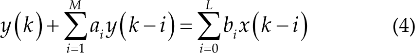
where x(k) and y(k) are the filter’s input and output, respectively, and M(≥ L) is the filter order, ai and bi are the parameters of the equation. The transfer function of the IIR filter can be written in the following general form:
Team-P continuously used 50, 20, 10, 30, and 40 Hz notch filters, respectively, and finally uses an 8th order Butterworth filter with an upper cut-off frequency of 0.72 Hz (Nyquist frequency) and a lower cut-off frequency of 0.008 Hz (Nyquist frequency) after baseline drift, and the corresponding real frequency is 1–90 Hz.
The relationship between Nyquist frequency and real frequency is given as follows:
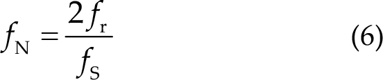
Here, fN is the Nyquist frequency, fr is the real frequency; fS is the sample frequency (250 Hz in the competition).
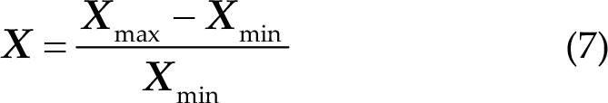
Team-B did not use a bandpass filter but used data standardization with the following equation:
Team-X uses a third-order Butterworth filter with an upper cut-off frequency of 0.32 Hz and lower cut-off frequency of 0.008 Hz, and the corresponding real frequency is 1–40 Hz.
Team-M also uses a third-order Butterworth filter with an upper cut-off frequency of 0.32 Hz and a lower cut-off frequency of 0.008 Hz, and the corresponding real frequency is 1–40 Hz.
2.2.2 Euclidean space alignment
Zanini et al. [19] proposed Riemannian alignment (RA), which is a transfer learning approach in the Riemannian space. The performance of the classifier with RA can be improved using the auxiliary data of other subjects with only a few labeled trials.
Specifically, RA first calculates the covariance matrices of some resting trials, where the subjects keep still. Then, it calculates the Riemannian mean

where ∑i is the covariance matrix of the ith trial, and
Inspired by RA, He et al. proposed EA, which does not need any labeled data from the new subject and can make the data distributions from different subjects more similar. The idea has been widely used in transfer learning [20–24]. The approach is also based on a reference matrix
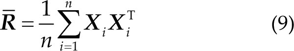
where

where
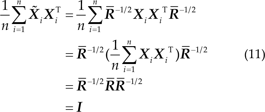
Thus, the mean covariance matrices of all subjects are equal to the identity matrix after alignment. Therefore, the distributions of the covariance matrices from different subjects are more similar, which is very desirable in transfer learning.
2.3 Non-deep learning framework
2.3.1 xDAWN
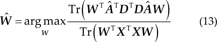
xDAWN is a spatial filtering approach that can find a transformation to improve the signal-to- noise ratio (SNR) of the ERP signal and reduce the dimension of the data [25].
The details of xDAWN are as follows: The EEG signal that contains the P300 component is
In reality, the P300 signal is assumed to be
The optimal filters
2.3.2 Tangent space mapping
Tangent space mapping maps a point on a Riemannian manifold into the Euclidean space, so that machine learning approaches in the Euclidean space can be applied.
First, the Riemannian mean
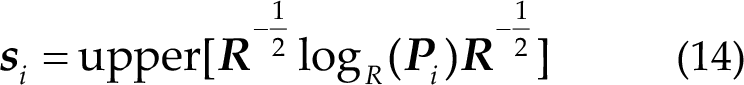
where the upper(·) means that the upper triangular part of the symmetric matrix is retained and vectorized, the weight of diagonal elements is 1, and the weight of other elements is
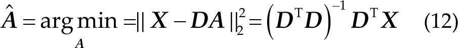
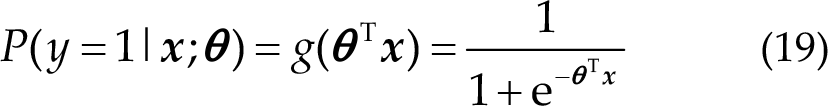
2.3.3 Logistic regression
Logistic regression is a machine learning approach for solving binary classification problems, which are used to estimate the possibility of classification.
The logistic and linear regression are generalized linear models. Logistic regression assumes that the dependent variable y follows the Bernoulli distribution, whereas linear regression assumes that the dependent variable y follows the Gaussian distribution. Therefore, it has many similarities with linear regression. Without a sigmoid activation function, the logistic regression algorithm is a linear regression.
In practice, linear regression is commonly used to fit the real data; the function is as follows:

Here,
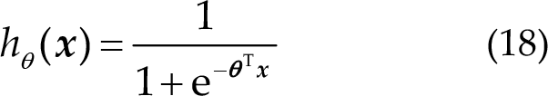
However, there are many data that do not obey the linear relationship. Thus, we use the sigmoid function to expand the use of hypothesis function. The sigmoid function introduces nonlinear factors into logistic regression, also known as logistic function:
where
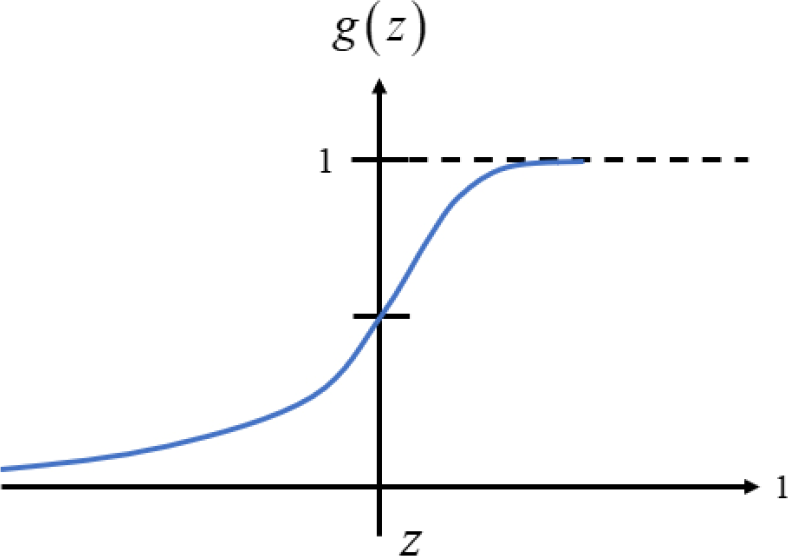
Sigmoid function.
Then, the form of hypothesis function is given as follows:
Therefore,
where
A machine learning model limits the decision function to a certain set of conditions, determining the hypothesis space of the model. The assumptions made by the logistic regression model are as follows:
The cost function in logistic regression J(θ) is given by
A better logistic regression model can be obtained by continuously optimizing the cost function.
2.4 Deep learning framework
2.4.1 LSTM
The LSTM network is a variant of a recurrent neural network (RNN). RNN can only have short-term memories because the gradient of the loss function decays exponentially with time (called the vanishing gradient problem). LSTM network combines short- and long-term memories through gate control, mitigating the vanishing gradient problem to a certain extent. It can learn long-term dependent information.
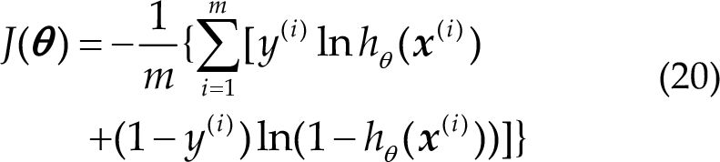
Figure 6 shows a schematic of RNN and LSTM. In the standard RNN, this repeated module has a very simple structure, such as a tanh layer. LSTM is the same structure but different from a single neural network layer. It has four neural network layers, with each having a specific purpose.
RNN and LSTM schematics. (a) RNN. (b) LSTM.
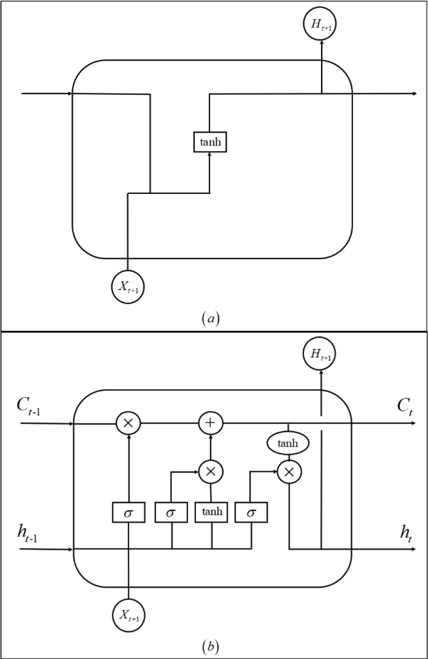
LSTM can remove or add information to the cell state because of the gate structure that contains a sigmoid neural network layer and a bitwise multiplication operation, as shown in Fig. 7.
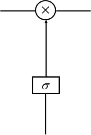
Gate structure of LSTM.
The sigmoid layer outputs a value between 0 and 1, describing how much each part can pass through. Here, 0 stands for “not allowed to pass any quantity”, and 1 stands for “allowed to pass all quantity”. More specifically, LSTM has three gates to control cell state. The first step in LSTM is to decide the information to forget from the cell state. The decision was made through a forget gate. The gate reads

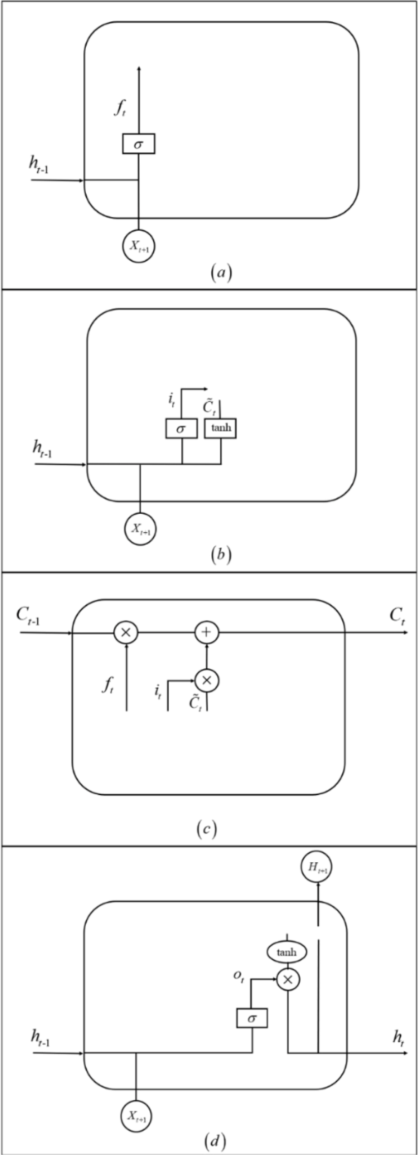
Meaning of the different parts of LSTM. (a) Forgetting information of LSTM. (b) Updating information of LSTM. (c) Updating cell state of LSTM. (d) Output information of LSTM.
Figure 8(b) shows the information to be updated:


Figure 8(c) shows the update cell state:

Figure 8(d) shows the output information:


Therefore, with the described architecture, LSTM can effectively process the time series data, such as EEG signal or Natural Language Processing (NLP) data, which studies the theory of communication between human and computer with natural language, such as machine translation, text classification, text semantic comparison and speech recognition.
2.4.2 EEGNet
EEGNet is a compact CNN architecture for EEG-based BCIs that: (1) can be applied in several different BCI paradigms, (2) can be trained with small data, and (3) can produce useful EEG features.
Figures 9 and 10 show a full description of the EEGNet model. EEG trials have C channels and T time samples. Lawhern et al. fit the model using Adam optimizer and cross-entropy loss function [26].
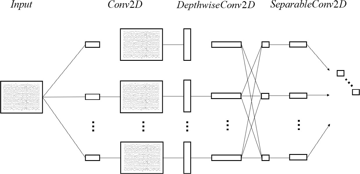
EEGNet architecture.
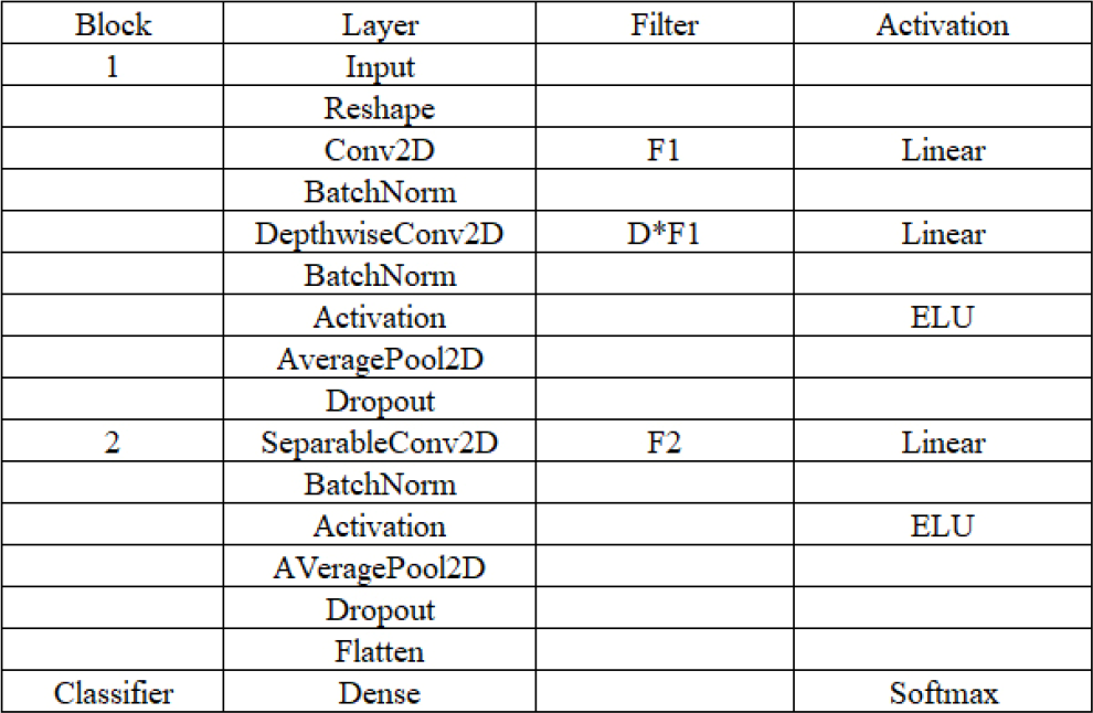
Network layer structure of EEGNet.
The first part of the network is time convolution, which can replace the frequency filter. The second part is a depthwise convolution, connecting to each feature map individually to learn frequency- specific spatial filters.
The third part is separable convolution. It combines depthwise and pointwise convolutions and collects a temporal summary from each feature map and optimally mixes all feature maps separately. Figure 10 shows the full details of the network architecture.
2.4.3 DeepConvNet
Robin et al. designed the DeepConvNet architecture inspired by successful architectures in computer vision, as described by Krizhevsky et al. [27].
DeepConvNet has four blocks, “Conv-Pool-block”. The first block has two convolution layers and max pooling with a special first block designed to handle EEG signal. The second, third, and fourth blocks consist of a convolution layer and a max pooling layer. The last layer is a dense softmax classification layer; the details are shown in Fig. 11. Figure 12 shows the parameters of DeepConvNet.
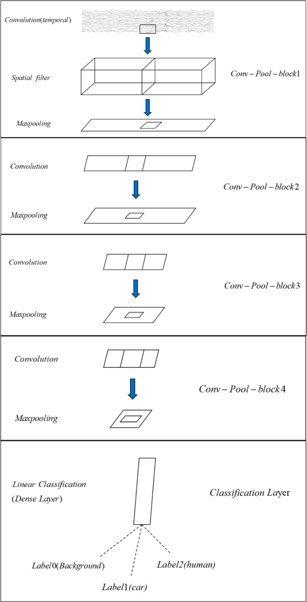
Conv-Pool-block of DeepConvNet.
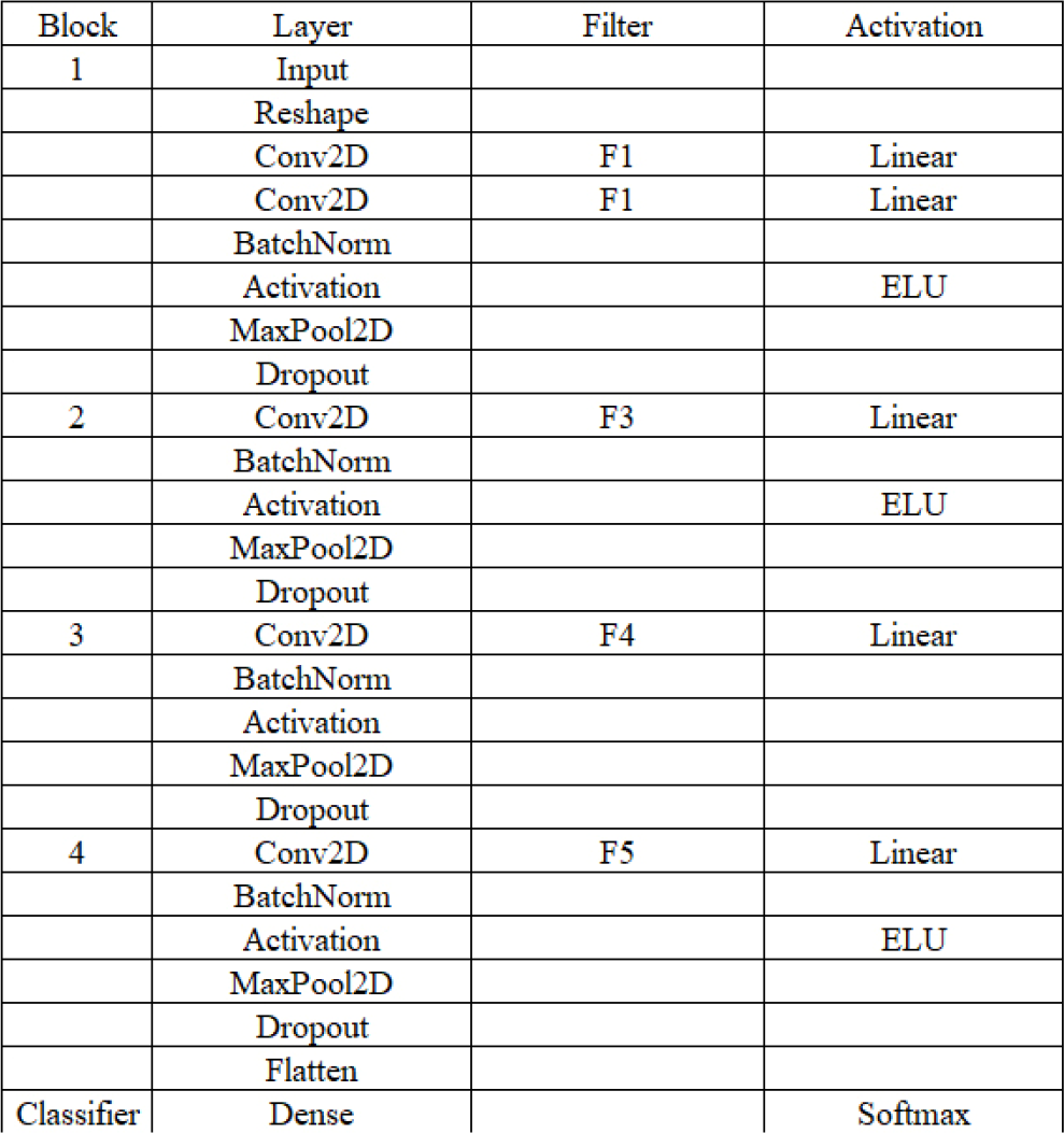
Network layer structure of DeepConvNet.
Especially, using two layers in the first block implicitly regularizes the overall convolution by forcing a separation of the linear transformation into a combination of a temporal convolution and a spatial filter.
2.5 Training strategy in training-free scenario
Although participants cannot obtain training data from subjects in the competition, they can use data from subjects in the preliminary. There are six different subjects in the preliminary competition, and the competition organizer provides 21 blocks for each subject.
The shape of the EEG data is (X,C,Y). Here, X is the number of trials, C is the number of channels, T is the time point length of the EEG data.
In Algo-H, participants use the non-deep learning framework to first divide the data into four-time point lengths of 125, 145, 165, and 185. Because there is a certain data imbalance in RSVP data, the ratio of the data with label 0 to data with labels 1 and 2 is 15:1. Thus, the idea of OvR (One vs. Rest) multi-classifier is used. The OvR classification strategy is to train N classifiers by taking samples of one category as positive examples and samples of all other categories as negative examples at a time. For example, the data with labels 1 and 2 are combined into one class, and the data with label 0 is set as one class separately. Therefore, two classifiers are used for the multi-classification problem. The first classifier separates 0 from (1, 2), and the second classifier separates 1 from 2. Therefore, there are eight classifiers for four-time point lengths. Participants use xDAWN and Tangent space as feature extraction, and the classifier is logistic regression. Figure 13(a) shows the details of Algo-H.
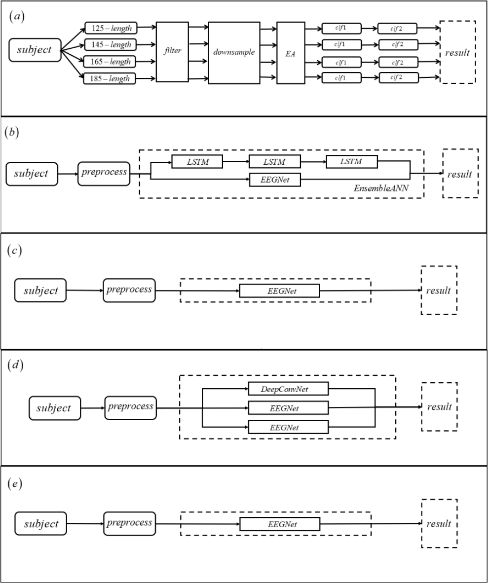
Flowcharts of the five algorithms. (a) Algo-H. (b) Algo-P. (c) Algo-B. (d) Algo-X. (e) Algo-M.
In Algo-P, participants used the deep learning framework. First, they used the notch filter of 50, 20, 10, 30, and 40 Hz. Second, they used the baseline detrend drift. Finally, they used the eight-order Butterworth filter. Furthermore, the participants combined three LSTM networks serially with the EEGNet network. Figure 13(b) shows the details of Algo-P.
In Algo-B, the participants used the deep learning framework. First, they used data standardization without any filter. Second, they reorganized the data with disrupting the channel order and reassembled the data into its original shape. Different subjects were trained and tested with EEGNet. Figure 13(c) shows the details of Algo-B.
In Algo-X, the participants used the deep learning framework. First, they used the third- order Butterworth filtering operation on the data. Then, they combined DeepConvNet with two EEGNet for training and testing. Figure 13(d) shows the details of Algo-X.
In Algo-M, the participants used the deep learning framework. First, they used the third- order Butterworth filter. Then, they trained with EEGNet, which is similar to the idea of Algo-B. Figure 13(e) shows the details of Algo-M.
3 Results
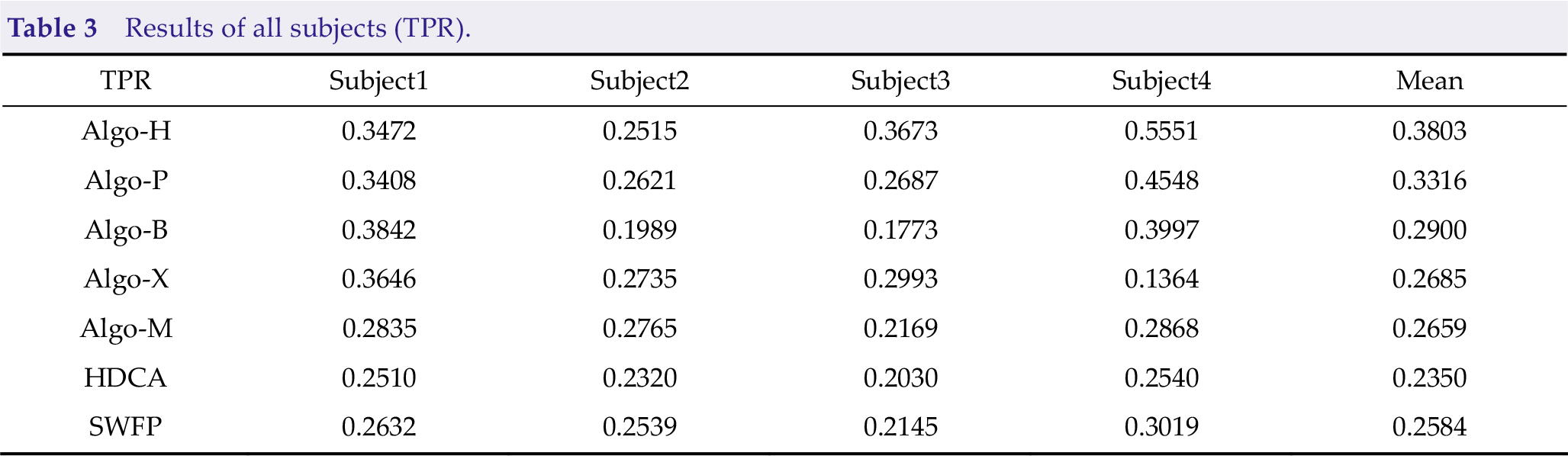
There were four subjects in the finals, and each subject had three blocks of data. Tables 3, 4, and 5 present the mean results on the four subjects of the algorithms. We added HDCA and SWFP [28–30] as the baselines. Different subjects have different results due to different environments and technical levels.
Results of all subjects (TPR).
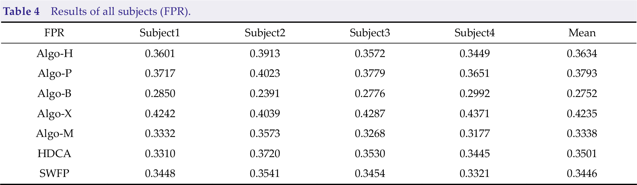
Results of all subjects (FPR).
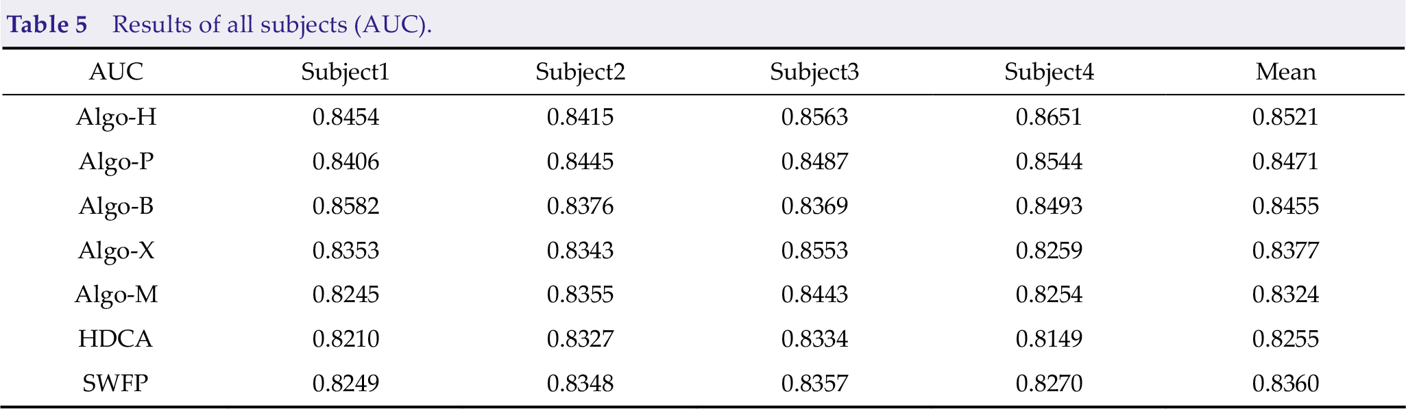
Results of all subjects (AUC).
The results of Subject4 were much higher than those of Subject1, Subject2, and Subject3. Algo-H performed much better than other algorithms on TPR. It also has an outstanding performance on subjects skilled with the instructions. In other words, the performance of Algo-H is more stable, meaning that a non-deep learning framework may be suitable for the scene.
Specific analysis is as follows: Too little training data may make the deep learning framework easy to overfit; meanwhile, the non-deep framework is naturally suitable for scenes with small data. Additionally, RSVP is a paradigm with unbalanced samples, where there are too many non-targets and few targets, easily leading to the problem of inaccurate classification boundary in the deep learning framework. However, the non-deep learning framework based on OvR is conducive to solving the problems because it classifies different tasks separately and improves accuracy. However, the deep learning framework can also achieve the best accuracy through an appropriate feature extraction approach.
Algo-B and Algo-M perform better than other algorithms on FPR. Specific analysis is as follows: Algo-B and Algo-M are algorithms with a single EEGNet, which makes the algorithms not have an extreme bias to predict the target results (label 0, label 1). Because of the use of a large number of classifiers, Algo-H uses OvR classifers, Algo-P uses EEG-Net and three LSTM Networks, and competitors use TPR to extremely optimize the algorithms so that the algorithms tend to predict the results with target labels 0 and 1.
Algo-H, Algo-P, and Algo-B perform better than other algorithms on AUC. Specific analysis is as follows: Algo-H and Algo-P perform better on TPR. However, Algo-B has advantages on FPR that its AUC is also good enough. In practice, keeping a balance between TPR and FPR is important to achieve better AUC. The competitors may use AUC to optimize the algorithms in the future because AUC can reflect the overall performance of the algorithm.
Figure 14 shows the TPR of all blocks. Some algorithms have good results in some subjects. However, it can be found that algorithms using more feature extraction and ensemble learning approaches can ensure better performance in multiple subjects, such as Algo-H and Algo-P.
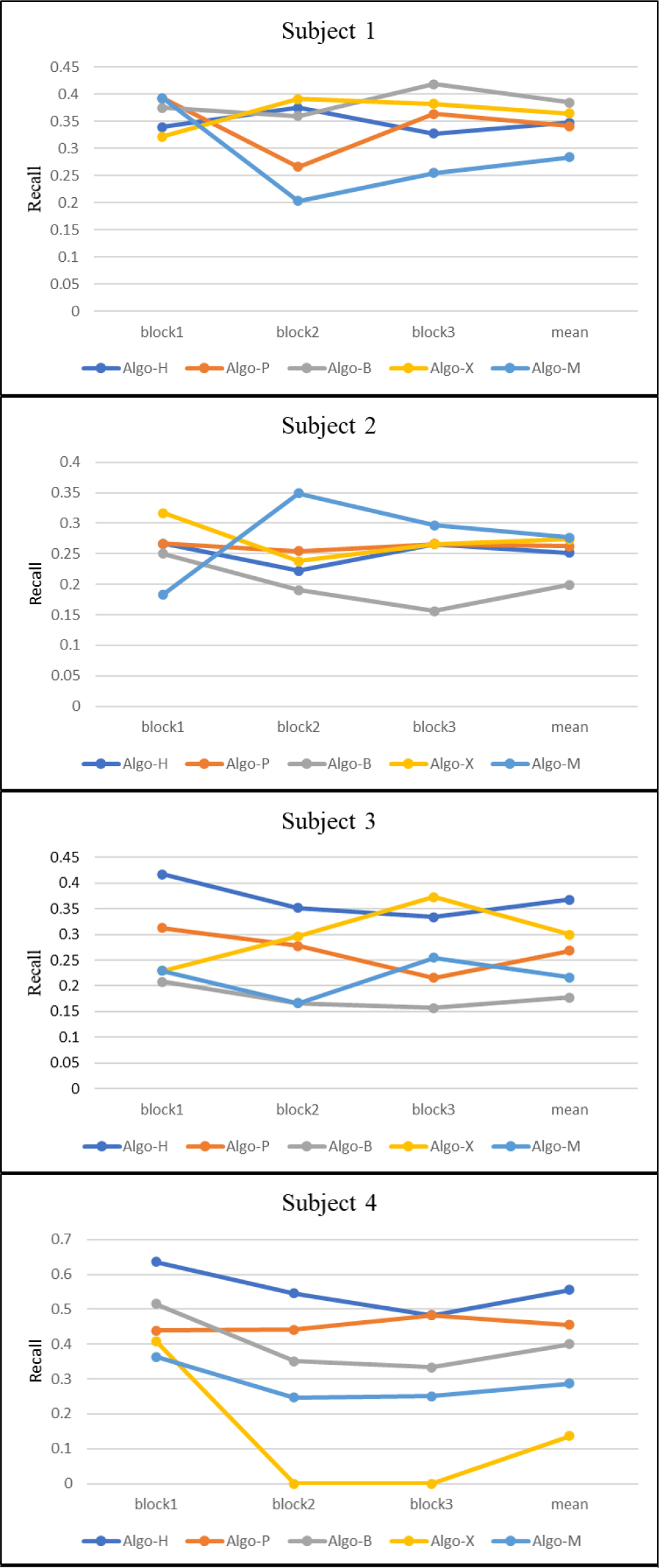
TPR of all blocks.
4 Discussion
This paper introduces the algorithm used by the top-five teams in the finals of the WRC2021 ERP competition. These algorithms use several new approaches to improve the performance of ERP in the training-free scenario.
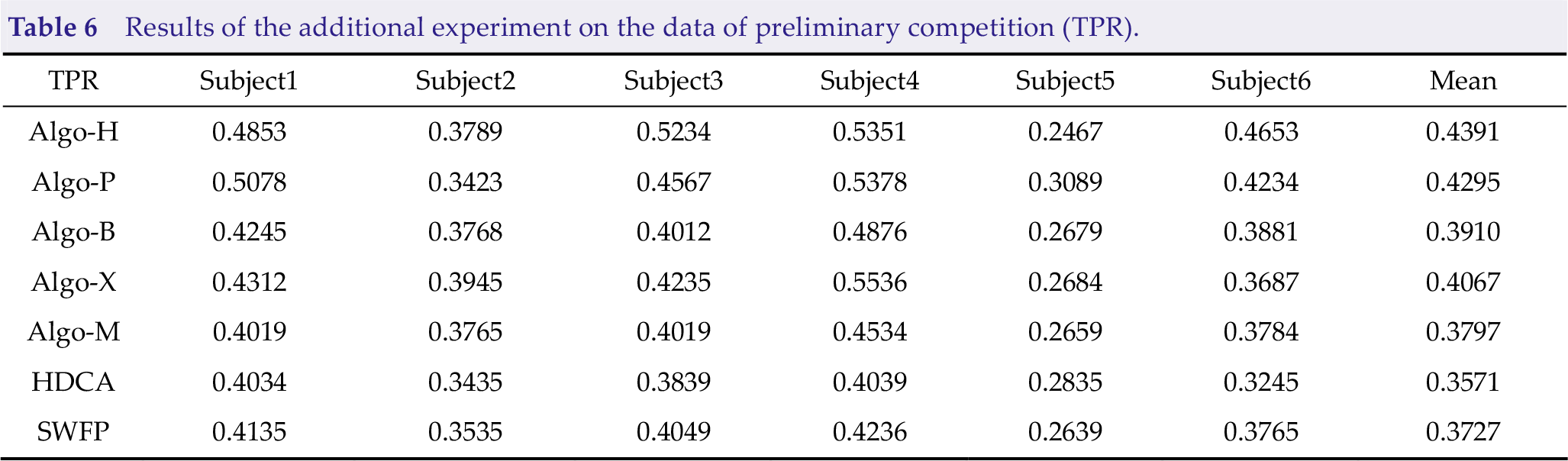
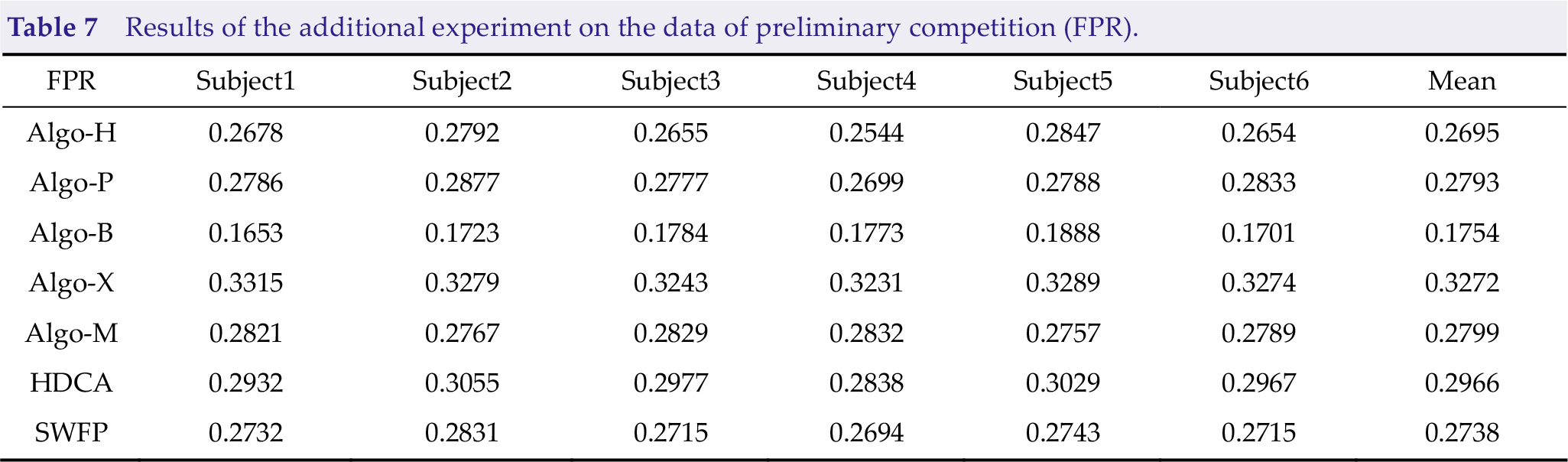
However, we cannot test whether these approaches are effective, and many models were pre-trained by preliminary data before the competition. Thus, we added an experiment based on data from the preliminary competition. Consequently, Algo-H, Algo-P, and Algo-B have good effects, as shown in Tables 6, 7, and 8.
Results of the additional experiment on the data of preliminary competition (TPR).
Results of the additional experiment on the data of preliminary competition (FPR).
Results of the additional experiment on the data of preliminary competition (AUC).
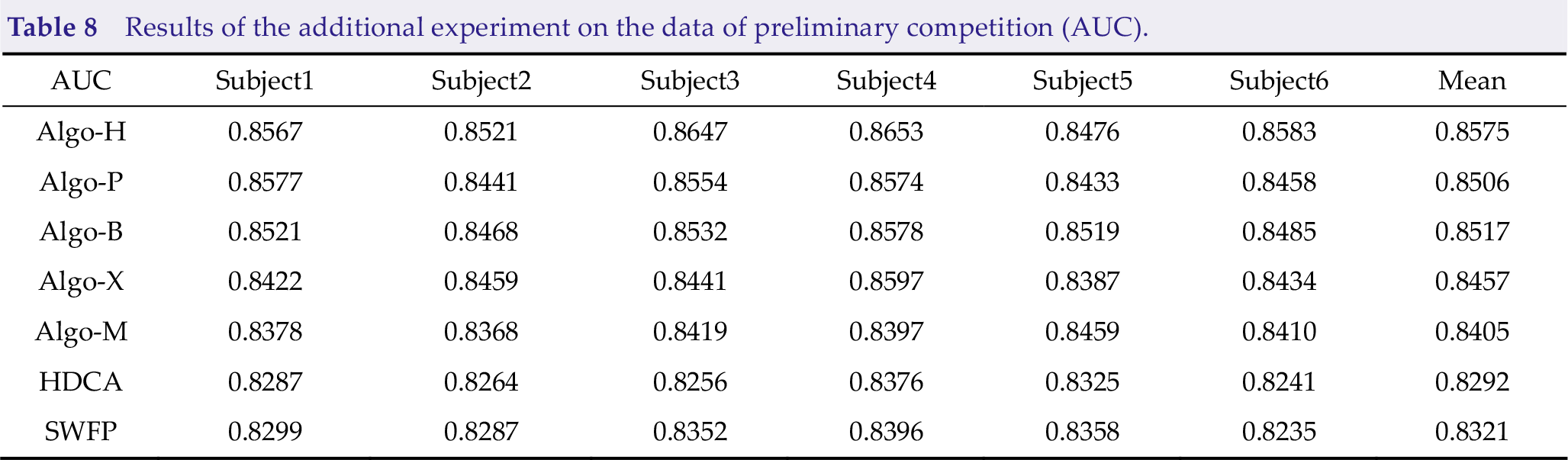
According to the results of the preliminary and final competitions, appropriate filtering approaches, data alignment, and feature extraction approaches can help the algorithm achieve better results; thus, determining the stability and generalization of the algorithm in training-free cross-subject scenarios. Algo-B and Algo-M use a single EEG as the classifier. Meanwhile, Algo-B uses the feature extraction approach to recognize the data; therefore, it has achieved better TPR on more subjects than Algo-M. However, whether the recombinant data adopted by Algo-B is reliable still needs more tests because it will reduce the algorithm performance on some subjects. Algo-H uses EA as a preprocessing approach, which is suitable for training-free scenarios.
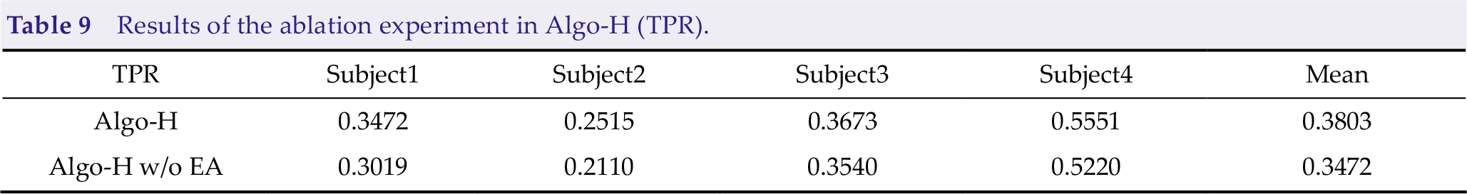
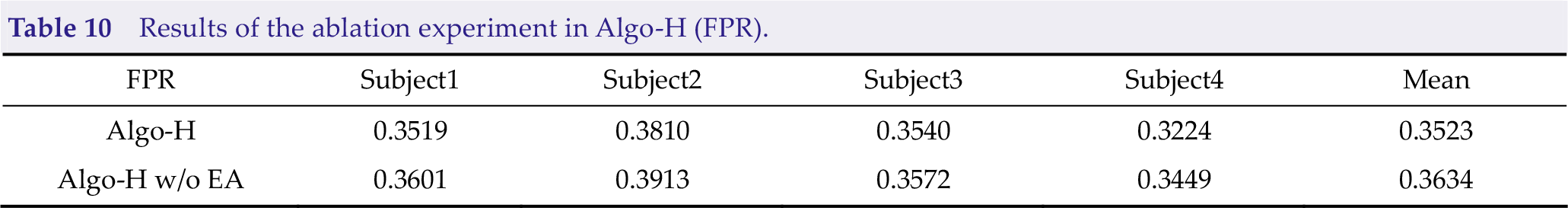
To confirm the effectiveness of EA, we added an ablation experiment of EA with Algo-H (Tables 9, 10, and 11). Thus, we obtained that EA could improve TPR and AUC up to 3.31% and 0.56%, respectively, and reduce FPR down to 1.11%.
Results of the ablation experiment in Algo-H (TPR).
Results of the ablation experiment in Algo-H (FPR).
Results of the ablation experiment in Algo-H (AUC).
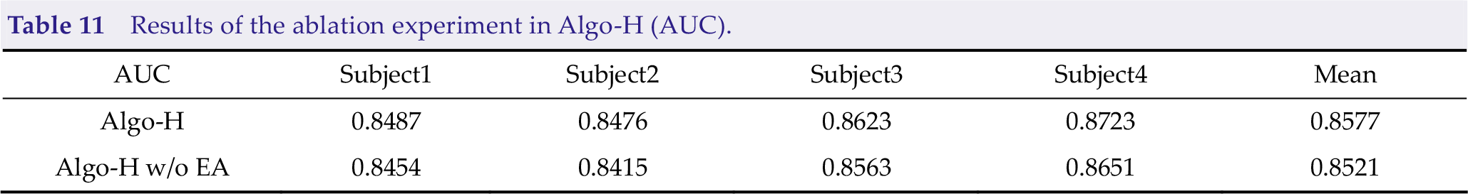
In terms of classifier, only Algo-H adopted non-deep learning approaches, such as logistic regression classification. The other four groups used neural networks. In the finals of the WRC2021 ERP competition, Algo-H achieved the best TPR on Subject3 (0.3673) and Subject4 (0.5551). It also achieved good TPR on Subject1 (0.3472) and Subject2 (0.2515). Meanwhile, Algo-B and Algo-P achieved the best TPR on Subject1 (0.3842) and Subject2 (0.2621), respectively.
Algo-B and Algo-M achieved good FPR on Subject2 (0.2391) and Subject3 (0.2776), and Algo-H (0.8521), Algo-P (0.8471), and Algo-B (0.8455) performed better in AUC.
Additionally, ensemble learning plays an important role in improving algorithm performance.
Algo-H uses different time points lengths to integrate, and Algo-P uses three LSTM networks to combine with the EEGNet network, which has achieved good results.
5 Conclusion
The described algorithms provide some new ideas for dealing with ERP training-free scenarios. For ERP, EA and appropriate filtering approaches can significantly improve algorithm performance because of the ablation experiment of Algo-H and the comparison of Algo-B and Algo-M. Additionally, the non-deep learning algorithm may be more stable than the deep learning approach. Ensemble learning can make the model more stable and robust. Furthermore, combining the non-deep learning approach and deep learning may have better performance. Keeping a balance between TPR and FPR is still essential to promote the model’s AUC. In future studies, we will test all algorithms on more diverse datasets to test the effectiveness of each approach. Then, we will propose a more comprehensive and practical training-free framework to improve the performance of the ERP analysis.
Footnotes
Conflict of interests
All contributing authors report no conflict of interests in this work.
Funding
This research was supported by the National Key Research and Development Program of China (Grant No. 2021ZD0201303), the Technology Innovation Project of Hubei Province of China (Grant No. 2019AEA171), and the Hubei Province Funds for Distinguished Young Scholars (Grant No. 2020CFA050).
Authors’ contribution
Conception and design of the study, data acquisition and analysis, manuscript drafting and revising: Huanyu Wu. Reviewing and approving the final draft of the manuscript: Huanyu Wu and Dongrui Wu.