Sage Journals: Discover world-class research

Abstract

This work aimed to measure the in vivo quantification errors obtained when ray-based iterative reconstruction is used in micro-single-photon emission computed tomography (SPECT). This was investigated with an extensive phantom-based evaluation and two typical in vivo studies using ^99mTc and ¹¹¹In, measured on a commercially available cadmium zinc telluride (CZT)-based small-animal scanner. Iterative reconstruction was implemented on the GPU using ray tracing, including (1) scatter correction, (2) computed tomography-based attenuation correction, (3) resolution recovery, and (4) edge-preserving smoothing. It was validated using a National Electrical Manufacturers Association (NEMA) phantom. The in vivo quantification error was determined for two radiotracers: [^99mTc]DMSA in naive mice (n = 10 kidneys) and [¹¹¹In]octreotide in mice (n = 6) inoculated with a xenograft neuroendocrine tumor (NCI-H727). The measured energy resolution is 5.3% for 140.51 keV (^99mTc), 4.8% for 171.30 keV, and 3.3% for 245.39 keV (¹¹¹In). For ^99mTc, an uncorrected quantification error of 28 ± 3% is reduced to 8 ± 3%. For ¹¹¹In, the error reduces from 26 ± 14% to 6 ± 22%. The in vivo error obtained with “^mTc-dimercaptosuccinic acid ([^99mTc]DMSA) is reduced from 16.2 ± 2.8% to −0.3 ± 2.1% and from 16.7 ± 10.1% to 2.2 ± 10.6% with [¹¹¹In]octreotide. Absolute quantitative in vivo SPECT is possible without explicit system matrix measurements. An absolute in vivo quantification error smaller than 5% was achieved and exemplified for both [”^mTc]DMSA and [¹¹¹In]octreotide.

ABSOLUTE QUANTIFICATION is very important in in vivo preclinical single-photon emission computed tomography (SPECT) because it enables the estimation of radioligand-specific binding kinetics, receptor density, and other relevant biologic parameters.¹ This can lead to faster drug development,² improved organ dose estimation accuracy,³ improved follow-up, and reduced variability in experimental design in microSPECT studies as the animals can serve as their own control⁴ in a longitudinal setting.

However, several issues can lead to inaccurate quantification. These errors, attributed to attenuation, scattering, partial volume effect (PVE), and system imperfections,⁵ can be compensated for within an iterative reconstruction framework.⁶ One approach is to measure the system response on a grid of discrete locations in the field of view (FOV).⁷ These measurements combine geometric response with more complex effects, such as detector variability and collimator imperfections. Although easy to measure in completely stationary systems, this is more difficult in rotating systems due to imperfect mechanical motion.⁸ A different approach is to directly incorporate the physical processes leading to these effects (eg, detector response, limited pinhole diameter, sensitivity) into ray-driven reconstruction.^9–11

Table 1 gives an overview of the current status of absolute quantification in preclinical SPECT. Seven recent articles compared ground-truth measurements to micro-SPECT results.^4,12–17 Wu and colleagues achieved a quantification error of 2 to 4.8% for ^99mTc and 3.7 to 9% for ¹¹¹In using system matrix measurements in their reconstruction.^12,14 With direct modeling, an error less than 10% was calculated regardless of the radioisotope used.^13,15–17 Lee and Chen studied the errors obtained from a parallel-hole setup and achieved low errors for ^99mTc (< 2%).¹³ However, filtered back projection was used to reconstruct their emission data.

Table 1.

Review of Recent Preclinical Quantification Errors Reported in the Literature

Isotope	System	Type of Study	Error (%)	Reference
Phantom experiments
^99mTc	X-SPECT (parallel hole)	Rat-sized uniform phantom	± 1.9	13
^99mTc	X-SPECT (parallel hole)	4-quarter phantom	2.2-3.4	13
^99mTc	X-SPECT (parallel hole)	Concentric phantom	± 2.0, ± 35.0	13
^99mTc	U-SPECT-II^*	Homogeneous phantom	–1.7	12
^99mTc	U-SPECT-II	Homogeneous phantom	4.8	14
^99mTc	U-SPECT-II	Point sources in ex vivo rat	–6.2 to 4.8	12
^99mTc	U-SPECT-II	Point sources in ex vivo rat	2.0	14
^99mTc	NanoSPECT/CT^†	3-vial phantom	< 10	15
^99mTc	Dual-head clinical camera, single pinhole	9-vial phantom	–5.1 to 1.2	16
^99mTc	Dual-head clinical camera, multipinhole	9-vial phantom	−0.3 to 4.1	16
¹¹¹In	U-SPECT-II	Homogeneous NEMA	9.1	14
¹¹¹In	U-SPECT-II	Point sources in ex vivo rat	3.7	14
¹¹¹In	NanoSPECT/CT	3-vial phantom	8-11	15
¹¹¹In	NanoSPECT/CT	Corning tubes with 2 inserts	± 5	4
¹²⁵I	U-SPECT-II	Homogeneous NEMA	−4.0	14
¹²⁵I	U-SPECT-II	Point sources in ex vivo rat	2.1	14
²⁰¹Tl	U-SPECT-II	Homogeneous NEMA	7.3	14
²⁰¹Tl	U-SPECT-II	Point sources in ex vivo rat	3.3	14
In vivo experiments
^99mTc	Dual-head clinical camera, multipinhole	In vivo mouse liver	−9.5 to −7.9	16
¹¹¹In	NanoSPECT/CT	In vivo rat kidney and liver	−9 and 9	4

CT = computed tomography; NEMA = National Electrical Manufacturers Association; SPECT = single-photon emission computed tomography.

MiLabs, Utrecht, The Netherlands.

†

Bioscan, Inc., Washington, DC.

Only three studies compared in vivo to ex vivo data.^4,15,16 Unfortunately, the data reported in those publications lack some aspects. In Vanhove and colleagues, a clinical dual-head system was used, retrofitted with a pinhole collimator.¹⁶ Direct modeling of attenuation and scatter reduced the quantitative error to −7.9 ± 10.4%. No PVE correction was applied, and no data are available for other isotopes. In Cheng and colleagues, the iterative reconstruction method was stopped well before convergence at only 24 maximum likelihood expectation maximization (MLEM) iterations, and no results were shown for ^99mTc.⁴ Lastly, Finucane and colleagues used uncorrected reconstructions.¹⁵

The aim of this work was to demonstrate the feasibility of in vivo absolute quantitative microSPECT using direct model-based corrections for ^99mTc and ¹¹¹In, alleviating the need to measure the system matrix for each isotope. Both isotopes encompass a range of photopeaks that serve as a good testing ground. The errors from a standard commercially available SPECT/computed tomography (CT) system with a multipinhole collimator are reported. All calibration and reconstruction implementations were not provided by the system vendor but were implemented by us.

For the in vivo study, we focused on these two tracers: ^99mTc-dimercaptosuccinic acid ([^99mTc]DMSA) and [¹¹¹In]octreotide. [^99mTc]DMSA is used to assess renal function^18,19 and, preclinically, is mostly used as an indicator of tubular functioning after ⁹⁰Y therapy.²⁰ A system resolution better than 1 mm is needed to delineate the functional renal cortex in mice,²¹ necessitating PVE correction and CT contrast agent to accurately delineate the kidneys. The second tracer, [¹¹¹In]octreotide, is a radioactively labeled octapeptide that pharmacologically mimics natural somatostatin. It is internalized in neuroendocrine tumors expressing somatostatin receptor type 2 (SSTR2) (and, to a lesser extent, SSTR3 and SSTR5).²²

Materials and Methods

System

All data were acquired on the trimodal FLEX Triumph-II system (TriFoil Imaging [formerly Gamma Medica Ideas], Northridge, CA). Its SPECT subsystem consists of one 80 × 80 pixel cadmium zinc telluride (CZT) detector head, equipped with a multipinhole collimator. The detector is 5 mm thick, and each pixel has a pitch of 1.6 mm (2.25 mm² active area). A five-pinhole collimator with 1.0 mm diameters was fitted 75 mm from the detector and positioned 55 mm from the axis of rotation, leading to an FOV of 68 mm per pinhole. Figure 1A depicts the amount of pinhole multiplexing.

Figure 1.

A, Overlap of individual pinhole projections, annotated with the number of overlapping pinholes in each region. B, Measured spectra of ^99mTc and ¹¹¹In. reduce the resulting Gibbs artifacts and smooth the images, an edge-preserving smoothing term was also incorporated, based on a bayesian rule penalty term.^26,27 The image denoising was weighted depending on each voxel belonging to significant edges or not,²⁷ such that volumes were not smoothed across anatomic boundaries. The edge map of the CT image was therefore first thresholded,²⁸ after which the neighboring voxels of edges were searched for.²⁷ Those neighbors form the areas wherein spillover may occur with conventional smoothing. This previous information was used in a one-step-late scheme to allow quadratic smoothing in edge-less areas, whereas the spillover areas were left unsmoothed.²⁷ We empirically set the regularization factor, which determines the magnitude of smoothing applied. All reconstructions ran for 50 iterations with 8 subsets²⁹ per iteration, reconstructing 120³ 0.5 mm × 0.5 mm × 0.5 mm voxels.

Because only one camera head is installed in our system instead of the possible four cameras, we doubled the acquisition time per view and doubled the injected dose. These two countermeasures led to a fourfold increase in collected data, as if the system had four heads. This resulted in a SPECT acquisition protocol using 64 views over a 360° total rotational angle, with an exposure of 2 minutes per projection view. All data were acquired in one bed position.

System Calibrations

List-mode output was acquired to obtain finer control over the conversions to sinograms. This allowed us to use our own developed software, without having to use the software included with the commercial system. The listmode output was converted into a sinogram by counting the detected events per pixel. Each detected event was decay corrected to the start of the SPECT acquisition. The channel number was converted to photon energy by applying a quadratic calibration equation. The equation coefficients were determined by least squares fitting channel numbers to the known photopeak energies of the radioisotopes ^99mTc and ¹¹¹In (including the 23 keV x-ray peak). The data were acquired from low-count point sources placed 1 m away from the uncollimated detector. This resulted in the following per pixel equation:

E = 1.4858 E - 5 V^{2} + 0.0719 V + 9.3624,

with V as the detected channel number and E as the calibrated energy value (keV). There is a clear nonlinear gain on the channel number, together with a baseline offset for the number of dark counts. The nonlinear gain is a compensation for the quadratic increase in electron cloud diameter at increasing photon energies.²³ Larger electron clouds lead to more charge sharing, which decreases the collected charge per pixel and thus the recorded energy. The resulting measured spectra are plotted in Figure 1B. The energy resolution was measured by fitting a gaussian function to the photopeaks acquired from the point source. In the case of the 171 keV peak from ¹¹¹In, the downscatter from the 245 keV peak was subtracted from the spectrum first. The downscatter was estimated by the average number of photons between 187 and 215 keV. The resulting energy resolution was 5.3% for 140.5 keV (^99mTc), 4.8% for 171.3 keV, and 3.3% for 245.4 keV (¹¹¹In).

The SPECT system geometry was further characterized by a multipinhole calibration method using three point-sources.^24,25

SPECT Reconstruction Including Corrections

Iterative Reconstruction Algorithm

As a starting point, all data were first reconstructed using the vendor-provided SPECT reconstruction software. This software is based on an ordered subset expectation maximization (OSEM) implementation. The data are precorrected for radioactive decay. The photopeak window width was always set to 10% of the photopeak energy. The OSEM reconstruction algorithm was used and was set to 10 iterations and 8 subsets, with a voxel size of 0.5 mm.

Next, the one-step-late ordered subset expectation maximization (OSL-OSEM) algorithm²⁶ was implemented in CUDA. A seven-ray pinhole diameter subsampling scheme was used to provide resolution recovery.^10,17 To

Scatter Correction

Scatter was measured during list-mode conversion, using the dual-energy window (DEW)³⁰ and the five-energy window (FEW) method³¹ for ^99mTc and ^mIn, respectively. The photopeak and scatter windows were empirically selected based on the calibrated spectra (Figure 1B), taking into account the asymmetrical peak. Table 2 shows the different energy windows used for each radioisotope. Photon scatter was corrected by adding the measured scatter to the forward-projected estimate inside the reconstruction algorithm. In scatter correction, usually a Butterworth filter is applied to smooth the scatter fraction³² to approximate the low-frequency nature of the scatter fraction. For the system under study here, we reduced the noise with a median filter (two-pixel radius) instead of the Butterworth filter.¹⁶ This filter is edge preserving and will not move data across pinhole boundaries in multiplexing systems.

Table 2.

Specific Technique and Scatter Windows Used for ^99mTc and ¹¹¹In

	Photopeak Window(s) (keV)	Scatter Window(s) (keV)	Technique
^99mTc	128–150	126–129	DEW²⁷
¹¹¹In	164–182; 238–256	160–168; 180–200; 236–239	FEW²⁸

DEW = dual-energy window; FEW = five-energy window.

Sensitivity Correction

Each three-dimensional sample measured in the projectors is corrected for a distance- and angle-dependent factor, taking an enlarged pinhole diameter into account due to photon penetration.^10,33 Detector sensitivity is implemented by attenuating the incoming ray with a factor dependent on the incidence angle and the attenuation of CZT for the isotope used.

Attenuation Correction

Attenuation was corrected for by using data acquired with the CT subsystem of the FLEX Triumph-II, mounted in the same gantry as the SPECT subsystem. This provides optimal hardware-based coregistration. All CT images were acquired on a 2,368 × 2,240 pixel detector (pitch 50 μm) using 512 views. A peak voltage of 75 kVp, exposure time of 345 ms, and tube current of 510 μA were chosen, with magnification X2, leading to a FOV of 59.2 × 56 mm. The total acquisition time was 13 minutes. All CT data were reconstructed using the maximum likelihood for transmission tomography (MLTR)³⁴ algorithm to a voxel matrix with isotropic voxel pitch of 100 μm, leading to an image with 592 × 592 × 560 voxels. The implementation uses the same ray-driven core as the SPECT reconstruction. The reconstructed images were bilinearly scaled³⁵ into attenuation values without coherent scattering as scatter correction was added separately. This high-resolution attenuation map was used directly in the forward projector.

Quantitative Calibration

One last calibration is needed to relate the reconstructed count density to the radioactivity concentration (MBq/mL). A small amount of known activity was scanned with the same protocol used during the other scans in this study. For ^99mTc, a point source of 10.61 MBq was used. The activity of the ^mIn point source was equal to 4.31 MBq. The scaling factor was calculated by dividing the known activity of the calibration vial by the total number of reconstructed counts times the volume per voxel.¹⁶ By multiplying a reconstructed image with such a scaling factor, an image with unit MBq/mL per voxel is obtained. The calibration vial was reconstructed without corrections as attenuation and scatter are assumed to be negligible due to the small volume size of a point source. For radioisotopes that emit photons in multiple photopeaks (eg, ¹¹¹In), each photopeak was first reconstructed separately with all possible correction factors enabled. After summing the final reconstructed images into a single image, it was multiplied by the scaling factor determined from the summed reconstructions of the calibration vial. As the scaling factor was determined from the total number of reconstructed counts, the isotope branching fraction is implicitly accounted for.

Phantom Experiments

The phantom design for the validation study is based on the image quality phantom described in the National Electrical Manufacturers Association (NEMA) NU 4-2008 specifications.³⁶ The phantom dimensions are illustrated in Figure 2. Two experiments were conducted to evaluate the quantitative accuracy for the two isotopes. The largest compartment was filled with a 1:1 ratio activity and the two smaller compartments with an 8:1 and 2:1 ratio. To allow delineation of all three compartments on the CT images, 0.375 mL iodine-based contrast agent (Visipaque 320 mg I/mL, GE Healthcare, Little Chalfont, Buckinghamshire, UK) was added to the 8:1 compartment, the 2:1 compartment received 0.750 ml contrast agent, and no contrast was added to the background compartment. Therefore, the radioisotope was first diluted with distilled water in a separate vial while weighing to obtain the correct concentrations. After measuring the concentration in the vial with the gamma counter, iodine contrast was added to this vial by pipetting the correct volume. If done beforehand, the iodine would attenuate the ground-truth gamma-counter measurements. Part of the contained volume was then used to fill the corresponding phantom compartment. The final activity concentrations can be found in Table 3. The technical specifications of the three compartments were used to select volumes of interest (VOI). These VOI were shortened axially to exclude air bubbles. This resulted in two cylindrical volumes of diameter 8 mm and height 5 mm for the 8:1 and 2:1 compartments and one cylindrical volume of diameter 30 mm and height 10 mm for the 1:1 compartment. The quantitative analysis consisted of measuring the mean activity in each compartment and comparing this to the known value.

Figure 2.

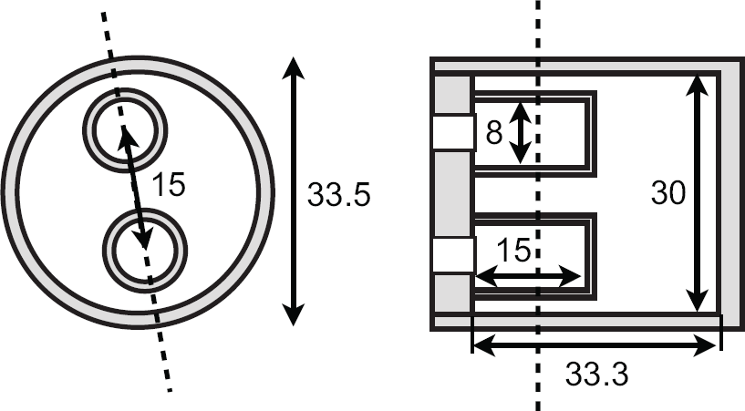
Technical specifications (units mm) for the SPECT quantification phantom. The dashed line is the location of the other cross-section view.

Table 3.

Dose Calibrator-Measured Activity Concentrations in the NEMA Phantom

Isotope	1:1 (MBq/mL)	2:1 (MBq/mL)	8:1 (MBq/mL)
^99mTc	2.84	6.03	21.05
¹¹¹In	2.95	4.51	18.38

NEMA = National Electrical Manufacturers Association.

In Vivo Small-Animal Imaging

Two in vivo studies were used to determine the absolute quantification error in realistic preclinical experiments. The Ghent University ethical committee approved all animal experiments (ECD 12/53).

[^99mTc]DMSA

BALB/c mice were selected with weight 26 ± 1 g and age 11 ± 1 wk (n = 6). Anesthesia was induced using 4% isoflurane; for maintenance of the anesthesia, the concentration was set at 1.7%. All mice were injected in the lateral tail vein with 78 ± 3 MBq [^99mTc]DMSA (TechneScan DMSA, Mallinckrodt Medical BV, Petten, The Netherlands). We aimed for a synchronous start of the SPECT scan 4.5 hours postinjection to maximize the uptake of the DMSA in the kidneys.²¹ To visualize the kidneys on the CT images, 1 hour before the SPECT scan, an iodine-based contrast agent (Visicover ExiTron V, Miltenyi Biotec, Bergisch-Gladbach, Germany) was injected into the lateral tail vein (4 μL/g). A pilot test had shown that such a protocol results in a maximal contrast increase in the kidneys between 30 and 60 minutes postinjection. Therefore, the microCT scan was started 30 minutes after administering the contrast agent. The 128-minute SPECT acquisition was started after the microCT scan was finished. Immediately following the SPECT scan, the animals were euthanized by cervical dislocation and a blood sample was taken by cardiac puncture. Both kidneys were dissected, rinsed with physiologic saline, dried, and weighed. Kidney weight was converted into volume by assuming a 1.05 g/mL density.³⁷ All samples were measured in a NaI(Tl) well-type gamma counter, calibrated with activity measured in the same dose calibrator as used for the in vivo experiment. The kidney VOI were determined by thresholding the kidneys on the reconstructed CT images. The total activity and volume inside the VOI were recorded. The reported activity then equals the VOI activity subtracted by the blood activity concentration times the vascular volume fraction (VVF) in a kidney at 0.27 mL/g kidney weight.³⁸ The kidney weight was determined from the same VOI volume.

[¹¹¹In]Octreotide

A human non-small cell lung carcinoma (NCI-H727) was chosen as a neuroendocrine tumor model. CD-1 nude mice (n = 10) (Charles River, France) were injected subcutaneously with 5 × 10⁶ cells in the right hind leg. The animals without a palpable tumor were euthanized 3 weeks after inoculation. All remaining mice (n = 6, age 13 ± 1 wk, weight 27 ± 2 g) were anesthetized and then injected with 31 ± 1 MBq [¹¹¹In]octreotide (Octreoscan, Covidien Belgium, Mechelen, Belgium) via the lateral tail vein. The microCT scan was started 23 hours postinjection, after which the 128-minute microSPECT scan was started.³⁹ Immediately following the SPECT scan, the animals were euthanized by cervical dislocation, and a blood sample was taken by cardiac puncture. The tumor was excised from the thigh and rinsed in physiologic saline, dried, and weighed. Tumor weight was converted into volume assuming a 1 g/mL density.⁴⁰ All samples were measured in a calibrated NaI(Tl) well-type gamma counter.

The CT image was used to delineate the boundaries of each tumor. The total activity and volume inside the VOI were measured. Because VVF is unknown for these tumors, we assumed a value of 5% mL/g tumor tissue.⁴¹ The reported activity then equals the reconstructed activity concentration subtracted by the blood activity multiplied by the VVF.

Data Analysis

All data were analyzed by comparing fully corrected data to the vendor's software and to our uncorrected data.

Uncorrected data refers to data corrected only for decay, geometric sensitivity, and quantitative calibration. The corrected data are always corrected for decay, geometric sensitivity, resolution recovery, edge-preserving smoothing, quantitative calibration, and the VVF, with additional attenuation correction and/or scatter correction. All VOI were analyzed using the open-source AMIDE software package (version 1.0.4).⁴² Quantification errors were calculated per VOI and then averaged. The paired t-test was used to quantify significant differences between the quantification from reconstructed data and the known ground-truth values. Furthermore, a Bland-Altman analysis was conducted to further evaluate the agreement between reconstructed values and ground-truth values.

Results

Phantom Measurements

Figure 3 shows a transaxial and a coronal slice through the reconstructed SPECT image obtained after applying all corrections for both isotopes. Figure 4 correlates the activity concentrations measured on the reconstructed images to the activity concentrations measured in the dose calibrator. The uncorrected data and the fully corrected data were fit with a dashed line and a full trend line, respectively.

Figure 3.

Reconstructed images of the NEMA phantom for (A) ^99mTc and (B) ¹¹¹In. The volumes of interest used in the evaluation are depicted in white.

Figure 4.

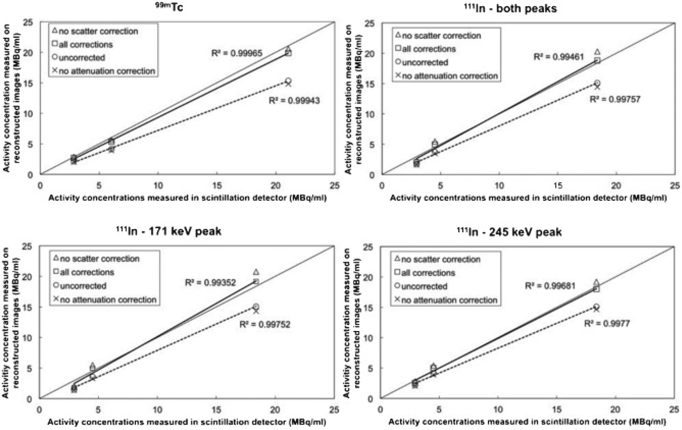
Correlation between the reconstructed and the ground-truth values for ^99mTc (top left) and ¹¹¹In (top right) with both peaks combined. The 171 keV and 245 keV peaks of ¹¹¹In are separated in the bottom row.

As can be seen from Figure 4, attenuation correction has the biggest influence on the quantitative accuracy. When all corrections were applied, except for scatter correction, the errors decreased on average from 2.78 ± 2.62 MBq/mL to 0.30 ± 0.25 MBq/mL for ^99mTc, from 1.91 ± 1.23 MBq/mL to −0.80 ± 1.66 MBq/mL for the low-energy peak of ¹¹¹In, and from 1.48 ± 1.58 MBq/mL to −0.53 ± 0.58 MBq/mL for the high-energy peak of ¹¹¹In. Combining both peaks leads to a decrease from 1.77 ± 1.34 MBq/mL to −0.72 ± 1.30 MBq/mL for ¹¹¹In, a small overcorrection. When all corrections are applied, including scatter correction, the quantification errors decrease from 2.78 ± 2.62 MBq/mL to 0.88 ± 0.85 MBq/mL for ^99mTc, from 1.91 ± 1.23 MBq/mL to −0.02 ± 1.04 MBq/mL for the low-energy peak of ¹¹¹In, and from 1.48 ± 1.58 MBq/mL to 0.08 ± 0.51 MBq/mL for the high-energy peak of ¹¹¹In. Combining both peaks decreases the error from 1.77 ± 1.34 MBq/mL to 0.01 ± 0.79 MBq/mL. Although these errors are low on average, a one-sample t-test of each value to the known reference value shows that each value is significantly different (p < .01) from the reference data, even after applying all corrections. The quantification errors for the separate vials are included in the summarized results in Table 4. Generally, a small undercorrection is found for ^99mTc, whereas the data for ¹¹¹In show a small overcorrection. For ¹¹¹In, the largest error can always be found in the 1:1 background vial.

Table 4.

Quantitative Errors Obtained from the NEMA Phantom with the Vendor-Provided Software and with Our Own Software, before and after All Corrections Were Applied

	1:1		2:1		8:1
	MBq/mL	%	MBq/mL	%	MBq/mL	%
^99mTc
Vendor	0.41 ± 0.70	14 ± 25	1.81 ± 1.29	30 ± 21	6.06 ± 3.53	29 ± 17
Uncorrected	0.71 ± 0.53	25 ± 19	1.90 ± 1.05	32 ± 17	5.73 ± 3.67	27 ± 17
Corrected	0.15 ± 0.66	5 ± 23	0.68 ± 1.29	11 ± 21	1.81 ± 4.36	9 ± 21
¹¹¹In
Vendor	1.16 ± 0.43	39 ± 15	0.70 ± 0.75	16 ± 17	3.52 ± 2.11	19 ± 11
Uncorrected	1.24 ± 0.37	42 ± 12	0.77 ± 0.49	17 ± 11	3.29 ± 1.64	18 ± 9
Corrected	0.92 ± 0.33	31 ± 11	−0.47 ± 0.67	−10 ± 15	−0.42 ± 1.94	−2 ± 11
¹¹¹In—low
Uncorrected	1.47 ± 0.32	50 ± 11	0.95 ± 0.47	21 ± 10	3.30 ± 1.64	18 ± 9
Corrected	1.16 ± 0.39	39 ± 13	−0.46 ± 0.76	−10 ± 17	−0.83 ± 2.03	−5 ± 11
¹¹¹In—high
Uncorrected	0.76 ± 0.31	26 ± 11	0.38 ± 0.50	8 ± 11	3.28 ± 1.79	18 ± 10
Corrected	0.39 ± 0.44	13 ± 15	−0.51 ± 0.68	−11 ± 15	0.36 ± 1.90	2 ± 10

NEMA = National Electrical Manufacturers Association.

Positive errors are undercorrections; negative errors are overcorrections.

Two-sample t-tests for the three different ¹¹¹In data sets (low, high, and combined photopeaks) show a significant difference for the three pairs for the 1:1 background vial, a significant difference between low and high for the 2:1 vial, and a significant difference for the 8:1 vial between low and high and between combined and low. The other combinations show no significant error difference.

In Vivo Small-Animal Imaging

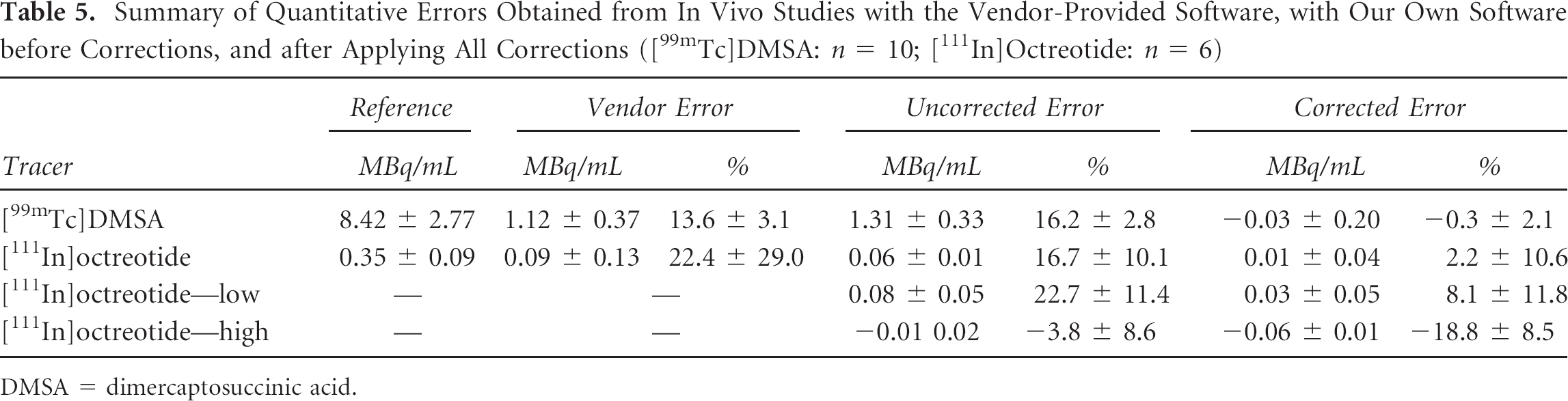
Figure 5 shows example reconstructions of the reconstructed in vivo data. Because of the difference in injected dose and tracer specificity, the background activity is much more of a confounding factor for [¹¹¹In]octreotide (see Figure 5B) than for [^99mTc]DMSA (see Figure 5A). Table 5 shows average absolute errors and average relative errors for both studies. For [¹¹¹In]octreotide, the separate quantification of each photopeak (low = 171 keV, high = 245 keV) is also included. Only 10 data points were available for [^99mTc]DMSA (instead of 12 kidneys harvested from 6 mice) as one acquisition failed due to the animal waking up during the SPECT scan.

Figure 5.

Reconstructed (A) [^99mTc] DMSA data and (B) [¹¹¹In]octreotide data. The tumor volume of interest is shown in yellow for data set B.

Table 5.

Summary of Quantitative Errors Obtained from In Vivo Studies with the Vendor-Provided Software, with Our Own Software before Corrections, and after Applying All Corrections ([^99mTc]DMSA: n = 10; [¹¹¹In]Octreotide: n = 6)

	Reference	Vendor Error		Uncorrected Error		Corrected Error
Tracer	MBq/mL	MBq/mL	%	MBq/mL	%	MBq/mL	%
[^99mTc]DMSA	8.42 ± 2.77	1.12 ± 0.37	13.6 ± 3.1	1.31 ± 0.33	16.2 ± 2.8	−0.03 ± 0.20	−0.3 ± 2.1
[¹¹¹In]octreotide	0.35 ± 0.09	0.09 ± 0.13	22.4 ± 29.0	0.06 ± 0.01	16.7 ± 10.1	0.01 ± 0.04	2.2 ± 10.6
[¹¹¹In]octreotide—low	—	—		0.08 ± 0.05	22.7 ± 11.4	0.03 ± 0.05	8.1 ± 11.8
[¹¹¹In]octreotide—high	—	—		−0.01 0.02	−3.8 ± 8.6	−0.06 ± 0.01	−18.8 ± 8.5

DMSA = dimercaptosuccinic acid.

The average activity reduction due to the VVF is 0.068 6 0.026 MBq for the [^99mTc]DMSA kidneys and 0.004 ± 0.003 MBq for the [¹¹¹In]octreotide tumors. A paired t-test indicated that there was no significant difference between the reference data and the fully corrected data whether the VVF was used or not. However, applying the VVF significantly (p < .01) decreased the quantification error for [^99mTc]DMSA from 0.038 ± 0.198 MBq/mL to −0.030 ± 0.201 MBq/mL. For [¹¹¹In]octreotide, a significant (p < .05) increase of 0.008 ± 0.040 MBq/mL to 0.012 ± 0.038 MBq/mL was found.

Figure 6 correlates the measured activity concentration to the reference ex vivo activity concentration. For [^99mTc]DMSA, there is a significant difference (paired t-test, p < .01) comparing the uncorrected data to the reference data, whereas the difference between fully corrected data and the same reference data is not significant (p = .64). Also for [¹¹¹In]octreotide, a paired t-test on the summed two-peak reconstruction shows a significant difference (p < .05) between the uncorrected and reference data, whereas no significant difference (p = .113) remained when comparing the corrected and the reference data. The goodness of fit improves when all corrections are applied but is worse for ¹¹¹In (R² = .778 and .823) than for ^99mTc data (R² = .991 and .995).

Figure 6.

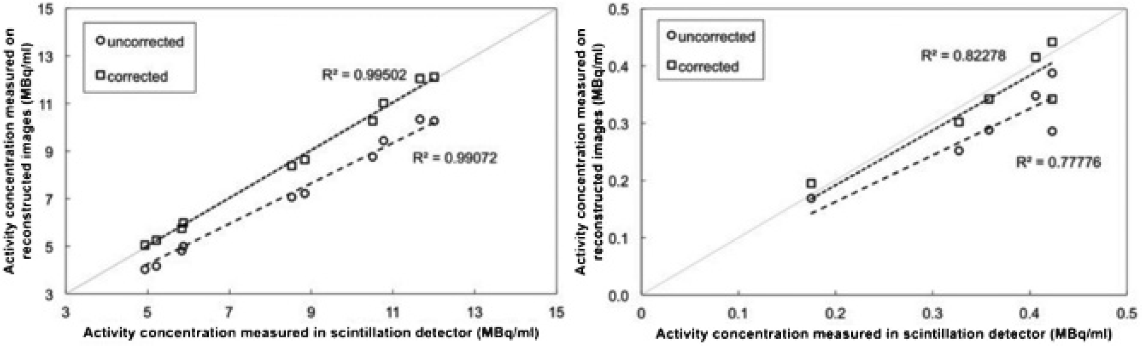
Quantification error for the [^99mTc]DMSA (left) and [¹¹¹In]octreotide (right) studies. The diagonal is the ground truth.

A Bland-Altman analysis is presented in Figure 7. A one-sample t-test to zero mean difference indicates a significant absolute systematic error for the difference between the uncorrected data and the reference data, for both isotopes (^99mTc: p < .01; ¹¹¹In: p < .05). This systematic error is relatively lower for ^99mTc than for ¹¹¹In. These results indicate a greater agreement between the reference and the corrected data than between the reference and the uncorrected data.

Figure 7.

Bland-Altman plots for (A) [^99mTc]DMSA and (B) [¹¹¹In]octreotide, comparing reference activity concentration and uncorrected reconstructed data (left) and reference activity concentration and corrected reconstructed data (right).

Discussion

Our study shows that a quantification error of less than 5% is achievable with ^99mTc and ¹¹¹In. This was accomplished with model-based iterative SPECT reconstruction on a standard, commercially available multipinhole microSPECT scanner. All data were reconstructed using direct physical modeling instead of system matrix measurements.

Our phantom results indicate that a decrease in quantification error is primarily influenced by attenuation correction. The influence of scatter correction is much smaller. This is partially caused by the CZT detector, which leads to a tail of low-energy events.⁴³ Thus, few scattered photons will be included in the photopeak window, at the expense of a lower amount of primary photons, increasing the statistical noise. This agrees with the findings of Chen and colleagues, who concluded that narrowing the energy windows is an effective way to correct for scatter in ^99mTc and ¹¹¹In studies, provided that sufficient energy resolution is available.⁴⁴ It should be stressed that scatter correction will increase in importance when other detectors are used (ie, with lower energy resolution) but will remain less important than attenuation correction in small-animal SPECT.⁶ This is also in agreement with the findings of Lee and Chen, who determined that attenuation is the prime factor to consider for this CZT-based system.¹³

Although the presented results are promising for routine use of absolute quantification in in vivo SPECT imaging, some issues were noticed during the experimental work. First, the importance of blood volume correction is not as clear as reported in Cheng and colleagues.⁴ Applying blood volume correction significantly changes the absolute quantification values. For [^99mTc]DMSA, this leads to a lower quantification error, whereas for [¹¹¹In]octreotide, the quantification error increases. This could be due to a misestimated blood volume for the H727 tumors. Although we measured the blood activity concentration by a heart puncture, a gamma-counting blood sampler can also be used. This was unavailable to us at the time. Few data of the VVF of different tissues are available, which makes this correction difficult in practice. One possible solution would be to directly measure the VVF using in vivo magnetic resonance imaging (MRI),^41,45 which would also account for intraspecies differences.

An important limitation of the DMSA study is the delineation of the renal cortex. The complete kidney was delineated and compared to the dissected complete kidney, instead of quantifying only the renal cortex. This was done because the renal cortex is still difficult to delineate on contrast-enhanced CT and because the cortex is also difficult to separate from the medulla during dissection. However, edge-preserving smoothing is still necessary to limit the overspill of activity in nonrenal tissue.

A second issue is the low system sensitivity in pinhole SPECT, which is combined with low biologic uptake in typical preclinical studies. The H727 cell line showed an uptake of only 1.4 ± 0.5% ID/g from [¹¹¹In]octreotide, resulting in an activity of 151 ± 40 kBq per tumor during the SPECT acquisition. The results obtained show that in vivo quantification is still possible at such a low activity, which is more than an order of magnitude lower than the activity reported by Finucane and colleagues,¹⁵ when normalized to the low sensitivity of our system.⁴⁶ Unfortunately, increasing the activity will not be possible for all tracers due to specific tracer kinetics (eg, irreversible binding).

Some system design ideas allow for pinhole systems with increased sensitivity. One is the multiplexing of pinholes, as is already used in the X-SPECT system. Several research groups have shown that multiplexing leads to image artifacts such as image nonuniformities and ghost activity due to the ambiguity of the projected data in overlapping regions.^47–51 A uniform phantom scanned with the X-SPECT system has already been shown to exhibit some nonuniformities (see Figure 8 in Deleye and colleagues⁴⁶) when a multipinhole collimator is used. However, the extent of multiplexing artifacts is dependent on the activity distribution and the geometric system design.⁴⁷ A similar nonuniformity was noticed in the uniform part of the phantom study (see Figure 3). This may influence the quantification error when only a small VOI is analyzed.

Conclusion

We have shown that absolute in vivo quantification is possible in microSPECT using direct modeling in iterative reconstruction, without the need for explicit measurements of the system matrix. An absolute in vivo quantification error smaller than 5% was achieved for two typical isotopes.

Footnotes

Acknowledgments

We would like to acknowledge Christophe Casteleyn and Lieselotte Moerman for their assistance during the experiments and Sara Rapic for neuroendocrine tumor implantations.

Financial disclosure of authors: This work was supported through a PhD grant awarded to Bert Vandeghinste by the Institute for the Promotion of Innovation through Science and Technology in Flanders (IWT-Vlaanderen) and by the iMinds CIMI project. Roel Van Holen is a postdoctoral research fellow of the Research Foundation Flanders (FWO) and part-time lecturer at Ghent University. Christian Vanhove holds a tenured assistant professor position within the GROUP-ID consortium of Ghent University. Stefaan Vandenberghe and Steven Staelens are associate professors granted by the Research Council of the universities of Ghent and Antwerp, respectively.

Financial disclosure of reviewers: None reported.

References

Almeida

Ribeiro

M-J

Bottlaender

. Absolute quantitation of iodine-123 epidepride kinetics using single-photon emission tomography: comparison with carbon-11 epidepride and positron emission tomography. Eur J Nucl Med 1999;26:1580–8, doi:10.1007/s002590050498.

Seo

. Quantification of SPECT and PET for drug development. Curr Radiopharm 2008;1:17–21, doi:10.2174/1874471010801010017.

Song

. A Monte Carlo and physical phantom evaluation of quantitative In-111 SPECT. Phys Med Biol 2005;50:4169–85, doi:10.1088/0031-9155/50/17/018.

Cheng

Rusckowski

Pretorius

. Improving the quantitation accuracy in noninvasive small animal single photon emission computed tomography imaging. Nucl Med Biol 2011;38:843–8.

King

Glick

Pretorius

. Attenuation, scatter, and spatial resolution compensation in SPECT. In: Wernick

Aarsvold

, editors. Emission tomography. London: Academic Press; 2004. p. 473–98.

Meikle

Kench

Kassiou

Banati

. Small animal SPECT and its place in the matrix of molecular imaging technologies. Phys Med Biol 2005;50:R45–61, doi:10.1088/0031-9155/50/22/R01.

van der Have

Vastenhouw

Rentmeester

Beekman

. System calibration and statistical image reconstruction for ultrahigh resolution stationary pinhole SPECT. IEEE Trans Med Imaging 2008;27:960–71, doi:10.1109/TMI.2008.924644.

Nuyts

Vunckx

Defrise

Vanhove

. Small animal imaging with multi-pinhole SPECT. Methods 2009;48:83–91.

Metzler

Jaszczak

Patil

. Molecular imaging of small animals with a triple-head SPECT system using pinhole collimation. IEEE Trans Med Imaging 2005;24:853–62, doi:10.1109/TMI.2005.848357.

10.

Accorsi

Metzler

. Analytic determination of the resolution-equivalent effective diameter of a pinhole collimator. IEEE Trans Med Imaging 2004;23:750–63, doi:10.1109/TMI.2004.826951.

11.

Smith

Jaszczak

. An analytic model of pinhole aperture penetration for 3D pinhole SPECT image reconstruction. Phys Med Biol 1998;43:761, doi:10.1088/0031-9155/43/4/006.

12.

van der Have

Vastenhouw

. Absolute quantitative total-body small-animal SPECT with focusing pinholes. Eur J Nucl Med Mol Imaging 2010;37:2127–35, doi:10.1007/s00259-010-1519-9.

13.

Lee

H-H

Chen

J-C

. Investigation of attenuation correction for small-animal single photon emission computed tomography. Comput Math Methods Med 2013;2013:1–13, doi:10.1155/2013/430276.

14.

de Jong

Gratama van Andel

. Quantitative multi-pinhole small-animal SPECT: uniform versus non-uniform Chang attenuation correction. Phys Med Biol 2011;56:N183–93, doi:10.1088/0031-9155/56/18/N01.

15.

Finucane

Murray

Sosabowski

. Quantitative accuracy of low-count SPECT imaging in phantom and in vivo mouse studies. Int J Mol Imaging 2011;2011:1–8, doi:10.1155/2011/197381.

16.

Vanhove

Defrise

Bossuyt

Lahoutte

. Improved quantification in single-pinhole and multiple-pinhole SPECT using micro-CT information. Eur J Nucl Med Mol Imaging 2009;36:1049–63, doi:10.1007/s00259-009-1062-8.

17.

Vanhove

Andreyev

Defrise

. Resolution recovery in pinhole SPECT based on multi-ray projections: a phantom study. Eur J Nucl Med Mol Imaging 2007;34:170–80, doi:10.1007/s00259-006-0225-0.

18.

Daly

Jones

Rudd

Tremann

. Differential renal function using technetium-99m dimercaptosuccinic acid (DMSA): in vitro correlation. J Nucl Med 1979;20:63–6.

19.

Yen

T-C

Chen

W-P

Chang

S-L

. Technetium-99m-DMSA renal SPECT in diagnosing and monitoring pediatric acute pyelonephritis. J Nucl Med 1996;37:1349–53.

20.

Forrer

Rolleman

Bijster

. From outside to inside? Dose-dependent renal tubular damage after high-dose peptide receptor radionuclide therapy in rats measured with in vivo 99mTc-DMSA-SPECT and molecular imaging. Cancer Biother Radiopharm 2007;22:40–9, doi:10.1089/cbr.2006.353.

21.

Jouret

Walrand

Parreira

. Single photon emission-computed tomography (SPECT) for functional investigation of the proximal tubule in conscious mice. Am J Physiol Renal Physiol 2010;298:F454–60, doi:10.1152/ajprenal.00413.2009.

22.

Reubi

J-C

Schar

J-C

Waser

. Affinity profiles for human somatostatin receptor subtypes SST1-SST5 of somatostatin radiotracers selected for scintigraphic and radiotherapeutic use. Eur J Nucl Med 2000;27:273–82, doi:10.1007/s002590050034.

23.

Kim

Anderson

Kaye

. Charge sharing in common-grid pixelated CdZnTe detectors. Nucl Instrum Methods Phys Res A 2011;654:233–43, doi:10.1016/j.nima.2011.06.038.

24.

Beque

Nuyts

Bormans

. Characterization of acquisition geometry of pinhole SPECT. IEEE Trans Med Imaging 2003;22:599–612, doi:10.1109/TMI.2003.812258.

25.

Vunckx

Defrise

Beque

. Geometrical calibration and aperture configuration design in multi-pinhole SPECT. In: 5th IEEE International Symposium on Biomedical Imaging: From Nano to Macro. Paris, France: Institute of Electrical and Electronics Engineers (IEEE); 2008. p. 1403–6.

26.

Green

. Bayesian reconstructions from emission tomography data using a modified EM algorithm. IEEE Trans Med Imaging 1990;9:84–93, doi:10.1109/42.52985.

27.

Vanhove

Defrise

Bossuyt

Lahoutte

. Improved quantification in multiple-pinhole SPECT by anatomy-based reconstruction using microCT information. Eur J Nucl Med Mol Imaging 2010;38:153–65, doi:10.1007/s00259-010-1627-6.

28.

Mortelmans

Nuyts

Pamel

. A new thresholding method for volume determination by SPECT. Eur J Nucl Med Mol Imaging 1986;12:284–90, doi:10.1007/BF00251989.

29.

Hudson

Larkin

. Accelerated image reconstruction using ordered subsets of projection data. IEEE Trans Med Imaginig 1994; 13:601–9, doi:10.1109/42.363108.

30.

Ogawa

Chugo

Ichihara

. Quantitative image reconstruction using position-dependent scatter correction in single photon emission CT. IEEE Nucl Sci Symp Conf Rec 1992; 2:1011–3, doi:10.1109/NSSMIC.1992.301459.

31.

Kint

Staelens

Vandenberghe

. Five energy window scatter correction for 111In microSPECT [abstract]. Society of Nuclear Medicine Annual Meeting Abstracts. J Nucl Med 2009;50 Suppl 2:293.

32.

Xiao

de Wit

Staelens

Beekman

. Evaluation of 3D Monte Carlo-based scatter correction for 99mTc cardiac perfusion SPECT. J Nucl Med 2006;47:1662–9.

33.

Smith

Jaszczak

. The effect of gamma ray penetration on angle-dependent sensitivity for pinhole collimation in nuclear medicine. Med Phys 1997;24:1701–9, doi:10.1118/1.597957.

34.

Nuyts

De Man

Dupont

Defrise

. Iterative reconstruction for helical CT: a simulation study. Phys Med Biol 1998;43:729–37, doi:10.1088/0031-9155/43/4/003.

35.

Brown

Bailey

Willowson

Baldock

. Investigation of the relationship between linear attenuation coefficients and CT Hounsfield units using radionuclides for SPECT. Appl Radiat Isot 2008;66:1206–12, doi:10.1016/j.apradiso.2008.01.002.

36.

NEMA NU 04-2008: performance measurements of small animal positron emission tomographs. Rosslyn, VA: National Electrical Manufacturers Association (NEMA); 2008. p. 1–30.

37.

International Commission on Radiological Protection. NEMA standards publication Nu4-2008. Basic anatomical and physiological data for use in radiological protection: reference values. Ontario: Elsevier Science; 2004.

38.

Sebestík

Brabec

Jelinek

Hlavata

. Red cell, plasma and whole blood volumes in organs of normal and hypersplenic rats. Blut 1974;29:203–9, doi:10.1007/BF01634123.

39.

Bernhardt

Kölby

Johanson

. Biodistribution of 111in-DTPA-D-Phe1-octreotide in tumor-bearing nude mice: influence of amount injected and route of administration. Nucl Med Biol 2003;30:253–60, doi:10.1016/S0969-8051(02)00417-1.

40.

Montelius

Ljungberg

Horn

Forssell-Aronsson

. Tumour size measurement in a mouse model using high resolution MRI. BMC Med Imaging 2012;12:12, doi:10.1186/1471-2342-12-12.

41.

Bremer

Mustafa

Bogdanov

. Steady-state blood volume measurements in experimental tumors with different angiogenic burdens—a study in mice. Radiology 2003;226:214–20, doi:10.1148/radiol.2261012140.

42.

Loening

Gambhir

. AMIDE: a free software tool for multimodality medical image analysis. Mol Imaging 2003;2:131–7. Available at: http://amide.sourceforge.net/.

43.

Volokh

Hugg

Blevis

. Effect of detector energy response on image quality of myocardial perfusion SPECT. IEEE Nucl Sci Symp Conf Rec 2008;4043–6, doi:10.1109/NSSMIC.2008.4774172.

44.

Chen

C-L

Wang

Lee

JJS

Tsui

BMW

. Toward quantitative small animal pinhole SPECT: assessment of quantitation accuracy prior to image compensations. Mol Imaging Biol 2008;11:195–203, doi:10.1007/s11307-008-0181-0.

45.

Persigehl

Wall

Kellert

. Tumor blood volume determination by using susceptibility-corrected R2* multiecho MR. Radiology 2010;255:781–9, doi:10.1148/radiol.10090832.

46.

Deleye

Holen

Verhaeghe

. Performance evaluation of small-animal multipinhole mSPECT scanners for mouse imaging. Eur J Nucl Med Mol Imaging 2013;40:744–58, doi:10.1007/s00259-012-2326-2.

47.

Mok

GSP

Wang

Tsui

BMW

. Quantification of the multiplexing effects in multi-pinhole small animal SPECT: a simulation study. IEEE Trans Nucl Sci 2009;56:2636–43, doi:10.1109/TNS.2009.2023444.

48.

Mok

GSP

Tsui

BMW

Beekman

. The effects of object activity distribution on multiplexing multi-pinhole SPECT. Phys Med Biol 2011;56:2635–50, doi:10.1088/0031-9155/56/8/019.

49.

Vunckx

Suetens

Nuyts

. Effect of overlapping projections on reconstruction image quality in multipinhole SPECT IEEE Trans Med Imaging 2008;27:972–83, doi:10.1109/TMI.2008.922700.

50.

Kench

Lin

Gregoire

M-C

Meikle

. An investigation of inconsistent projections and artefacts in multi-pinhole SPECT with axially aligned pinholes. Phys Med Biol 2011;56:7487–503, doi:10.1088/0031-9155/56/23/010.

51.

Lin

. On artifact-free projection overlaps in multi-pinhole tomographic imaging. IEEE Trans Med Imaging 2013;32:2215–29, doi:10.1109/TMI.2013.2277588.

Use of a Ray-Based Reconstruction Algorithm to Accurately Quantify Preclinical MicroSPECT Images

Abstract

Materials and Methods

System

System Calibrations

SPECT Reconstruction Including Corrections

Iterative Reconstruction Algorithm

Scatter Correction

Sensitivity Correction

Attenuation Correction

Quantitative Calibration

Phantom Experiments

In Vivo Small-Animal Imaging

[111In]Octreotide

Data Analysis

Results

Phantom Measurements

In Vivo Small-Animal Imaging

Discussion

Conclusion

Footnotes

Acknowledgments

References

[¹¹¹In]Octreotide