Magnetic Resonace–Based Attenuation Correction for Micro–Single-Photon Emission Computed Tomography

Abstract

Attenuation correction is necessary for quantification in micro–single-photon emission computed tomography (micro-SPECT). In general, this is done based on micro–computed tomographic (micro-CT) images. Derivation of the attenuation map from magnetic resonance (MR) images is difficult because bone and lung are invisible in conventional MR images and hence indistinguishable from air. An ultrashort echo time (UTE) sequence yields signal in bone and lungs. Micro-SPECT, micro-CT, and MR images of 18 rats were acquired. Different tracers were used: hexamethylpropyleneamine oxime (brain), dimercaptosuccinic acid (kidney), colloids (liver and spleen), and macroaggregated albumin (lung). The micro-SPECT images were reconstructed without attenuation correction, with micro-CT-based attenuation maps, and with three MR-based attenuation maps: uniform, non-UTE-MR based (air, soft tissue), and UTE-MR based (air, lung, soft tissue, bone). The average difference with the micro-CT-based reconstruction was calculated. The UTE-MR-based attenuation correction performed best, with average errors ≤ 8% in the brain scans and ≤ 3% in the body scans. It yields nonsignificant differences for the body scans. The uniform map yields errors of ≤ 6% in the body scans. No attenuation correction yields errors ≥ 15% in the brain scans and ≥ 25% in the body scans. Attenuation correction should always be performed for quantification. The feasibility of MR-based attenuation correction was shown. When accurate quantification is necessary, a UTE-MR-based attenuation correction should be used.

THE NECESSITY OF attenuation correction in clinical single-photon emission computed tomography (SPECT) studies has been extensively studied. Different authors have shown that the application of attenuation correction in clinical SPECT imaging improves diagnostic accuracy.^1–3 In recent years, it has become clear that attenuation correction should also be considered in small-animal micro-SPECT. In fact, attenuation correction is even more important in the case of small-animal imaging as in many micro-SPECT studies, the quantification of the activity in a lesion is more important than the detection of lesions (contrary to clinical imaging). This is illustrated by, for example, preclinical cancer studies with inoculated tumors: the location of the tumor is well known, and the researcher is interested only in quantification of the uptake in the tumor. Hwang and colleagues demonstrated that performing no attenuation correction can lead to a quantification error of 25% in preclinical imaging with ^99mTc labeled tracers. ⁴ If low-energy single-photon emitters such as ¹²⁵I are used, the error can be up to 50%. They also showed that implementation of attenuation correction into an iterative reconstruction algorithm can remove this error.

For attenuation correction, an attenuation map of the object under study is needed. Two options can be considered for the determination of the attenuation map: the attenuation map can be derived from the emission data, or the attenuation map can be measured separately. As some micro-SPECT tracers have uptake only in a specific organ, it is difficult to derive the attenuation map from the emission data in micro-SPECT. The attenuation map is often derived from x-ray computed tomographic (CT) images, but in theory, any imaging modality can be used. In the ideal case, the attenuation map will perfectly reflect the attenuation properties of the object under study. In the case of a small animal, this implies that a nonuniform attenuation map is used as the animal contains different tissue types, which have different attenuation properties. The main tissue types that can be discriminated, ranging from strongly attenuating to mildly attenuating, are bone, soft tissue, and lung. Although it is technically not a tissue, air should also be considered. It does not attenuate significantly and can be found at different locations throughout the body.

The most straightforward method to measure the nonuniform attenuation map is to use an imaging modality that measures tissue density. The first methods for performing attenuation correction in a clinical setting were based on transmission imaging. ⁵ Different studies have also shown the feasibility of CT-based attenuation correction for clinical SPECT.^6,7 In small-animal imaging, micro-CT can be used, as shown by Hwang and Hasegawa and Vanhove and colleagues.^8,9 This implies that the micro-CT values have to be rescaled to attenuation coefficients at the photon energy of the isotope used for the micro-SPECT scan. ¹⁰ Micro-CT has the advantage of also being able to provide an anatomic reference frame for the micro-SPECT images, which contain only limited anatomic information if a specific tracer is used. Micro-CT scans can be fast if the resolution requirements are modest.

There are two disadvantages to the use of micro-CT. First, micro-CT delivers poor contrast within soft tissue. Using large amounts of intravenous contrast agent can help this. This leads in turn to problems in the attenuation map as the attenuation coefficients of the contrast agents cannot be rescaled in the same way as biologic tissue. Bonta and Wahl showed that this leads to significant errors in the reconstructed image for clinical SPECT studies, but the effect on preclinical imaging has not been studied. ¹¹ It should be noted that high doses of contrast agent can also be toxic for the animals. Second, the dose delivered to the animal can be quite high (> 0.1 Gy). It has been proposed that this could affect the study outcome in longitudinal studies, which use many micro-CT scans.^12–15 The dose could have an effect on, for example, tumor metabolism or the immune system of the animal.

The attenuation map could also be derived from images acquired with magnetic resonance imaging (MRI). MRI has the advantage of delivering no radiation dose, and with the right sequence, it can deliver excellent soft tissue contrast. Therefore, it does not have the same disadvantages as micro-CT. However, the derivation of the attenuation map from MRIs is not as straightforward as it is from micro-CT images. The magnetic resonance (MR) properties of tissue are determined by a combination of proton density and relaxation properties. These are not directly correlated with tissue density. Extra problems are caused by the fact that both lung tissue and bone have no measurable signal when using conventional MR sequences. This is caused by low proton density and very fast relaxation, leading to destruction of the signal before it can be measured.

With the advent of the first preclinical and clinical scanners that combine positron emission tomography (PET) or SPECT with MRI, some research has been done into derivation of the attenuation map from MRIs.^16–19 We have previously shown the feasibility of deriving the attenuation map from MRI acquired with an ultrashort echo time (UTE) sequence for human brain PET. ²⁰ The UTE sequence provides signal in bone and lung by a special acquisition scheme. We validated our method in five clinical brain PET data sets. In this study, we used a comparable method to determine the attenuation map of a rat. The difficulty of deriving the attenuation map and the effect of errors in the attenuation map can depend on the region that is being imaged. Therefore, we evaluated our method on micro-SPECT studies of the brain, kidneys, liver and spleen, and lungs. In the following sections, the setup of the experiments and the micro-SPECT, micro-CT, and MRI is first described. Then the method used for deriving different attenuation maps from micro-CT and MRI is explained. The results from a comparison between micro-SPECT images reconstructed with micro-CT-based attenuation correction and MR-based attenuation correction are reported. A statistical analysis of the average activity concentration obtained with different attenuation correction methods is also described.

Materials and Methods

Acquisitions

Animal Preparation

Eighteen Hsd:Wistar rats were imaged. All rats weighed approximately 300 g and were no older than 8 weeks. Different radiotracers were used for micro-SPECT imaging. All radiotracers were administered via the tail vein. For the brain study, five rats were injected with 330 MBq of ^99mTc-labeled hexamethylpropyleneamine oxime (HMPAO). Thirteen rats were imaged for the body studies. Five rats were injected with 110 MBq of ^99mTc-labeled dimercaptosuccinic acid (DMSA, kidney tracer), five rats were injected with 300 MBq of ^99mTc-labeled colloids (liver and spleen tracer), and five rats were injected with 150 MBq of ^99mTc-labeled macroaggregated albumin (MAA, lung tracer). Of the rats injected with colloids, two died before the MRI acquisition could be finished, so only the results from three colloid scans are presented here. The rats were anesthetized with an intraperitoneal dose of 115 μL per 100 g body weight pentobarbital. This dose was slightly higher than the normal dose (100 μL per 100 g body weight) to keep the animals anesthetized long enough to perform all acquisitions.

Micro-SPECT and Micro-CT Acquisitions

Micro-SPECT imaging was done on a dual-head Siemens e.cam clinical gamma camera (Siemens Medical Systems, Erlangen, Germany) using two multipinhole collimators. Each collimator had three pinholes with 1.5 mm knife-edge pinhole apertures. Sixty-four projections were acquired over 360° into a 128 × 128 matrix using a detector pixel size of 4.8 mm. The radius of rotation of the system was 80 mm. The total micro-SPECT acquisition time was 30 minutes. The field of view (FOV) was cylindrical, with an approximate diameter of 55 mm and an axial length of 160 mm. The resolution of the system is 2.7 mm in a large central part of the FOV (up to a distance of 30 mm from the center). The system is described in more detail in Vanhove and colleagues. ²¹ The rats were then moved to the micro-CT scanner in the adjacent room while remaining on the same bed. A micro-CT scan was acquired on a SkyScan 1178 high-throughput in vivo micro-CT system (Skyscan, Kontich, Belgium). X-ray projections were acquired into a 1,280 × 1,024 matrix with two detector-source pairs, obtaining 196 projections over 212°. The CT settings were 50 kV and 615 μA. The acquisition time for the micro-CT was 2 minutes. The images were reconstructed with the software provided by the scanner manufacturer into a 1,024 × 1,024 × 1,024 matrix with 0.083 mm isotropic voxel size.

MR Acquisitions

MR acquisitions were performed on a clinical MR system (Philips Achieva 3T, Philips Medical Systems, Best, the Netherlands). A standard wrist coil was used for the brain scans. A standard knee coil was used for the body scans. The implemented UTE acquisition delivers two images. The first image is acquired at the first echo time (T_E1) very quickly after radiofrequency excitation (≈ 0.15 ms). It is not an actual gradient echo image but an image reconstructed from the free inductive decay (FID) signal. As this image is acquired before the signal in bone and lung is lost, the image intensities in voxels containing bone or lung are nonzero. The second image is a gradient echo image acquired at the second echo time (T_E2). This image can be compared to a conventional T₁-weighted MRI and will thus have very low signal in lung and bone. For more details about the UTE acquisition, see the Methods section of Keereman and colleagues. ²⁰

For the brain scans, UTE-MRIs were acquired at an isotropic resolution of 0.5 mm and with T_E1 and T_E2 set to 0.15 and 2.4 ms, respectively. Two averages were acquired to improve the signal to noise, yielding a total acquisition time of 35 minutes for an FOV of 75 mm × 75 mm × 75 mm. For the body scans, the resolution was 0.7 mm and a larger FOV was acquired to include almost the complete body of the rat (75 mm × 75 mm × 177 mm). Only one average was used to keep the acquisition time acceptable (40 minutes).

Registration

Micro-SPECT, micro-CT, and MR images were registered using rigid registration methods. To restrict movement when moving the rats between different scanners, the rats were placed inside a plastic tube before the start of the experiment. Two small syringes filled with water were also placed inside the plastic tube to help with the registration. The registration of micro-SPECT and micro-CT images was done using two circular disks placed on the bed used for both modalities. Each disk contained three 3.7 MBq ⁵⁷Co point sources. The method is described and validated in Vanhove and colleagues. ⁹ As the ⁵⁷Co point sources are not visible on MRIs, the same method could not be used for the MRIs. The MRIs were registered to the micro-CT images using A Medical Image and Data Examiner (AMIDE) ²² by selecting fiducial markers on both CT and MR images and applying the implemented alignment wizard. Different fiducial markers were used for the brain scans and the body scans. For the brain scans, three anatomic fiducial markers were used: the tip of the nose and the entrances of the left and right ear canals. Four fiducial markers were used for registration of the body scans: both ends of the water syringes placed inside the plastic tube. After registration, the micro-CT and MR images were resampled to the same matrix as the micro-SPECT images. This was a matrix of 128 × 128 × 128 voxels with an isotropic voxel size of 0.5 mm for the brain scans and a matrix of 128 × 128 × 256 with the same isotropic voxel size for the body scans.

Attenuation Maps

The goal of this study is to compare different methods of MR-based attenuation correction to the currently used attenuation correction on the system (micro-CT-based attenuation correction). Therefore, different attenuation maps were derived. All attenuation maps described in this section, derived for one of the DMSA (kidney) scans, are shown in Figure 1, C to F. As all micro-SPECT imaging was done with ^99mTc, attenuation coefficients for 140 keV photons were used.

Figure 1.

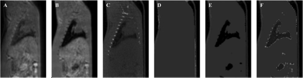
Free inductive decay image (A), gradient echo image (B), micro-CT-based attenuation map (C), uniform MR-based attenuation map (D), MR-based attenuation map discriminating air and soft tissue (E), and UTE-MR-based attenuation map discriminating air, lung, soft tissue, and bone (F) for one of the body scans.

First, the micro-CT-based attenuation map was derived. As micro-CT-based attenuation correction is currently the best available method for attenuation correction in micro-SPECT imaging, we can consider this attenuation map as the reference. The micro-CT image is first downsampled to the resolution of the micro-SPECT image by summing several neighboring voxels together. This also acts as a smoothing operator and reduces noise in the micro-CT. The attenuation map is then derived from the micro-CT image by rescaling the micro-CT value in each voxel according to the following formula:

$\mu \left({\text{cm}}^{-1}\right)=0.15\frac{\mathrm{I}}{{\mathrm{I}}_{\text{water}}}$

(1)

where I is the micro-CT value in the voxel and ^Iwater is the micro-CT value of water, which is calibrated daily. The micro-CT values obtained from the scanner are positive values with air = 0 and increase with measured tissue density. This formula then yields a linear scaling from the attenuation measured by CT to the attenuation coefficient for 140 keV photons. A linear scale was used rather than a bilinear scale (used, for example, in CT-based attenuation correction for PET) as Brown and colleagues showed that the relationship between CT values and attenuation coefficients is linear to a good approximation for low energies up to 140 keV. ²³

Three attenuation maps were derived from the MRIs, each using a different segmentation approach. Two of them can be derived from a conventional (non-UTE) MRI. In our study, the second (gradient echo) image of the UTE acquisition was used for this because it is a normal T₁-weighted MRI. A uniform (contour) attenuation map was derived by using region growing to determine the contour of the animal and setting the attenuation coefficient inside the contour to 0.15 cm⁻¹. A second attenuation map discriminating only soft tissue and air was extracted from the gradient echo image by simple thresholding. As there is no signal in the lungs in this image, this means that voxels in the lungs will be assigned air attenuation coefficients (0 cm⁻¹). Theoretically, this should also happen in voxels containing bone, but this was not the case, as reported in the Discussion section. The second attenuation map was not derived for the brain scans; as there is no lung tissue in the head, this attenuation map would be identical to the contour attenuation map.

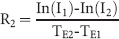
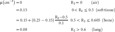
From the UTE images, information about bone and lungs can also be extracted. An extra attenuation map that discriminates air, lung, soft tissue, and bone was therefore also derived. This was done in three steps, which are summarized in Figure 2. First, the R₂ map was calculated. R₂ is the transverse relaxation rate. This is the inverse of the transverse relaxation time T₂, which is a well-known MR property of tissues. R₂ will be high in tissues with fast relaxation (bone, lung) and low in tissues with slow relaxation (soft tissue). It can be calculated voxel by voxel from both UTE images:

${\mathrm{R}}_2=\frac{\text{In}\left({\mathrm{I}}_1\right)-\text{In}\left({\mathrm{I}}_2\right)}{{\mathrm{T}}_{\text{E2}}-{\mathrm{T}}_{\text{E1}}}$

(2)

where I₁ and I₂ are the image intensities in the FID and gradient echo images and T_E1 and T_E2 are the echo times. Because the FID image is a low-quality image, it can contain noise or artifacts in voxels containing air. As this will not be the case in the gradient echo image, this can lead to a very high R₂ in these voxels. This was corrected by multiplying the R₂ map with a binary mask in which all voxels containing air were set to 0. This binary mask was derived from the FID image by thresholding, setting all voxels above the noise level to 1 and the rest to 0. The noise level was determined by taking the maximum value in a region of interest outside the rat body.

Figure 2.

Image processing steps used to derive an attenuation map from ultrashort echo time magnetic resonance images. FID = free inductive decay.

In this corrected R₂ map, different tissues are discriminated based on their R₂ value. Lung has the highest R₂, followed by bone. Soft tissue has a low R₂, and the R₂ in air is set to 0 by the binary mask. The UTE-MRI-based attenuation map was derived from the corrected R₂ map by applying a mapping to the R₂ values:

$\begin{array}{lll}\mu \left({\text{cm}}^{-1}\right)& =0& {\mathrm{R}}_2=0(\text{air})\\ & =0.15& 0<{\mathrm{R}}_2\le 0.5(\text{soft tissue})\\ \begin{array}{l}\\ \end{array}& \begin{array}{l}=0.15+(0.25-0.15)\frac{{\mathrm{R}}_2-0.5}{0.1}\\ =0.08\end{array}& \begin{array}{l}0.5<{\mathrm{R}}_2\le 0.605(\text{bone})\\ {\mathrm{R}}_2>0.6(\text{lung})\end{array}\end{array}$

(3)

The R₂ ranges of the different tissue types were taken from the results in Keereman and colleagues. ²⁰ The voxels with R₂ values between 0.5 and 0.6 should all contain bone, but they are not just assigned a single bone attenuation coefficient. This is done for two reasons. First, the contrast between bone and soft tissue was not always high enough to clearly discriminate both tissue types (the proposed reasons for this are explained in the Discussion section). Second, not all voxels containing bone have the same attenuation coefficient: on the micro-CT scan, a large range of values can be seen in bone. To compensate for both effects, the R₂ values between 0.5 and 0.6 are rescaled to the range of values between the attenuation coefficient of soft tissue (0.15 cm⁻¹) and the maximum attenuation coefficient of bone on the micro-CT-based attenuation maps (0.25 cm⁻¹). The linear scale that is used is a working assumption and has not been verified experimentally. The attenuation coefficient for voxels containing lung tissue was set to the average attenuation coefficient of lung tissue in the micro-CT-based attenuation maps.

The bed used for micro-CT and micro-SPECT and the plastic tube used to fixate the animals also caused some attenuation. As the bed is not MR compatible, it was not used for the MR scans and hence is not visible on the MRIs. The plastic tube was used in the MR scans but was also not visible on the MRIs as it provides no MR signal. Therefore, an attenuation template was made of the bed and tube from a CT scan of the bed and tube without an animal. The template was then included in every MR-derived attenuation map.

SPECT Reconstruction

The SPECT projections were reconstructed using an iterative reconstruction algorithm based on the ordered subsets expectation maximization (OSEM) algorithm.^21,24 The reconstructed matrix was 128 × 128 × 256 with an isotropic reconstructed voxel size of 0.5 mm. The algorithm models the system geometry as accurately as possible, taking into account the pinhole geometry, the collimator response, the angular variation of the sensitivity for each pinhole aperture, the intrinsic spatial resolution of the gamma camera, attenuation, and scatter. It is described in detail in Vanhove and colleagues. ⁹ The nonuniform attenuation correction was implemented in the iterative reconstruction as proposed by Gullberg and colleagues. ²⁵ A triple energy window (TEW) scatter correction was used. The SPECT images were reconstructed with four different attenuation maps: micro-CT based, MR uniform (contour) map, MR map with air and soft tissue, and a UTE-MR map with air, lung, bone, and soft tissue. A fifth reconstruction with no attenuation correction was also done.

Analysis

Vanhove and colleagues showed that the reconstruction algorithm yields absolutely quantitative results when using a nonuniform micro-CT-based attenuation map. ⁹ Therefore, the micro-SPECT images reconstructed with a micro-CT-based attenuation map can be considered the reference. Thus, in our study, we compared the images reconstructed with the micro-CT-based attenuation correction and the other images to prove that quantification is also possible with MR-based attenuation correction. This was done in two ways. First, the average percent difference ΔX in a volume of interest (VOI) was calculated:

$\Delta \mathrm{X}(\%)=100\frac{1}{\mathrm{N}}{\sum }_{\mathrm{i}}\frac{\left|{\mathrm{S}}_{\mathrm{X},\mathrm{i}}-{\mathrm{S}}_{\text{CT},\mathrm{i}}\right|}{{\mathrm{S}}_{\text{CT},\mathrm{i}}}$

(4)

where i is the voxel index, S_CT,i and S_X,i are the reconstructed SPECT activity concentrations in the image corrected with the micro-CT-based attenuation map and the other image, respectively, and N is the total number of voxels in the VOI. For the body scans, the VOI was automatically defined by thresholding on the micro-SPECT image reconstructed with the micro-CT-based attenuation map, taking into account only voxels that have a significant SPECT image intensity. This was done to avoid corruption of the results by voxels that have only very low tracer uptake. The threshold was set to 10% of the maximum micro-SPECT value. This was not done for the brain scans as HMPAO is a less specific tracer than the others. For the brain scans, the VOI was manually defined by a box that contained the complete brain.

Second, the average activity concentration in the different micro-SPECT images reconstructed with MR-based attenuation maps was compared to the images reconstructed with the micro-CT-based attenuation map. The significance of the difference between the average activity concentrations was tested using a paired Student t-test. The same VOIs as above were used for the evaluation. A significant difference was defined as a p value smaller than .05.

Results

Attenuation Maps

Figure 3 shows images of one of the brain scans. The UTE-MRIs (FID and gradient echo), the micro-CT-based attenuation map, the uniform MR-based attenuation map, and the MR-UTE-based attenuation map are depicted. Figure 1 shows the same images for one of the DMSA (kidney) scans but also includes the MR-based (non-UTE) attenuation map, which discriminates only air and soft tissue. The uniform MR-based attenuation maps (see Figure 1D and Figure 3D) are easy to derive, and the contour of the body is correctly defined. The same applies to the non-UTE-MR map, where lung tissue is assigned air attenuation coefficients (see Figure 1E). The bones in this image are segmented as soft tissue because of the issues discussed below.

Figure 3.

Free inductive decay image (A), gradient echo image (B), micro-CT-based attenuation map (C), uniform MR-based attenuation map (D), and UTE-MR-based attenuation map (E) for one of the brain scans.

The UTE-MR map of the brain shows a resemblance to the micro-CT-based attenuation map. Although the segmentation is not perfect, the large bone structures are discriminated in this attenuation map. The skull, jaw, and spine can be seen. The attenuation map derived from the body UTE-MRI shows good resemblance to the micro-CT scan in the lungs and soft tissue. The segmentation of the bones is more difficult. Although bone is detected in the ribs, the detected volume of bone is much smaller than on the micro-CT scan.

Reconstructed SPECT Images

For each type of scan, a slice of all SPECT images of a single rat reconstructed with different attenuation maps is shown in Figure 4. The grayscale window was the same within each scan type. Only very small visual differences can be seen between the micro-SPECT images reconstructed with the different attenuation maps (see Figure 4). The quantitative comparison shows more differences. The results for the brain scans should be interpreted separately from the body scans as the setting is clearly different. In the brain scans, the UTE-based attenuation correction performs best in all rats, yielding an average error in all rats of 5 to 8%. Uniform attenuation correction gives slightly larger errors, leading to errors above 10% in two subjects. No attenuation correction gives errors of around 15%. In the body scans, the average errors are much smaller. All MR-UTE-based attenuation maps have an average percent difference of 3% or less. The non-UTE-MR maps have an average percent difference of at most 6%. Large average errors between 25 and 45% are found when no attenuation correction is done. A summary of these results, grouped per scan type, is shown in Figure 5.

Figure 4.

SPECT images from different tracers reconstructed with different attenuation maps. Tracers from top to bottom: hexamethylpropyleneamine oxime (brain), dimercaptosuccinic acid (kidney), colloids (liver and spleen), and macroaggregated albumin (lung). Attenuation map from left to right: micro-CT-based, uniform MR-based, non-UTE-MR-based (air and soft tissue), and UTE-MR-based (air, lung, soft tissue, and bone). The third attenuation map was not used for the brain scans.

Figure 5.

Average percent difference with micro-CT-based attenuation correction in the reconstructed SPECT images, per scan type. The different attenuation maps are color coded. DMSA = dimercaptosuccinic acid; HMPAO = hexamethylpropyleneamine oxime; MAA = macroaggregated albumin. *Nonsignificant difference.

The average difference in activity concentration between the different MR-based attenuation correction methods and the CT-based attenuation correction is shown in Table 1. For the brain scans, all MR-based attenuation correction methods yield significant differences. For the body scans, the UTE-based attenuation correction yields a nonsignificant difference for all different tracers. The uniform MR-based attenuation correction leads to significant differences for all tracers except colloids.

Table 1.

Average Difference between Activity Concentrations Yielded by Different MR-Based Attenuation Correction Methods and Micro-CT-Based Attenuation Correction

	UTE-MR (%)	Non-UTE-MR (%)	Uniform MR (%)	None (%)
DMSA	0.59*	2.23	1.55	32.32
Colloids	0.61*	1.75*	1.08	26.56
MAA	0.60*	4.34	2.34	22.79
HMPAO	6.34		9.60	17.66

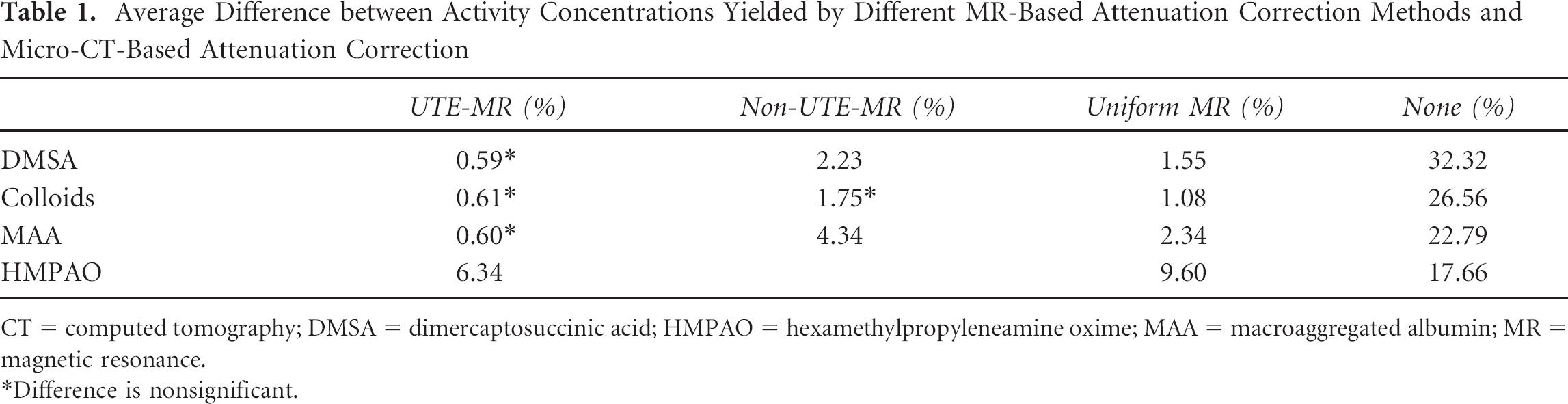
CT = computed tomography; DMSA = dimercaptosuccinic acid; HMPAO = hexamethylpropyleneamine oxime; MAA = macroaggregated albumin; MR = magnetic resonance.

*

Difference is nonsignificant.

Discussion

When looking at both UTE images, it is clear that the FID image is of lower general quality than the gradient echo. The FID body image (see Figure 1A) in particular looks more blurred and exhibits more noise. This can be seen clearly around the edges of the body. The reasons for the lower quality of the FID image are manifold, and a thorough discussion is not within the scope of this article. However, care should always be taken to acquire good UTE images and use optimized scanner settings. These images also show why applying the binary mask is necessary. If the R₂ map was used in its uncorrected form, there would be a lot of voxels with a high R₂ surrounding the body. By applying the binary mask, these voxels are set to 0 in the corrected R₂ map.

The UTE acquisition provides signal in bone and lung as the image intensity in the FID image in these tissues is well above the noise level. This is in clear contrast to the gradient echo image. The image intensity in the lungs in Figure 1B is almost zero. In the brain image (see Figure 3B), the drop in signal is also apparent in the bones of the skull, spine, and jaw. This will lead to high R₂ values. There is also a signal drop in bone in the body image (see Figure 1B), but it is much smaller than in the brain image. This is because the ribs are smaller than the MR resolution. This leads to partial volume effects in voxels containing soft tissue and bone. The soft tissue relaxes much more slowly than the cortical bone and remains visible in the gradient echo. In the end, this leads to a lower contrast between soft tissue and bone in the gradient echo and the R₂ map. Bone will thus be segmented as soft tissue from these images. For the attenuation correction, this is much better than segmenting bone as air as the attenuation coefficient of bone is much closer to soft tissue than to air. Bone is also detected in regions where no bone is present. The most obvious is the contour of the lungs. Partial volume effects comparable to what happens with bone and soft tissue will lead to lower R₂ values at the border of the lungs, where lung and soft tissue are contained in the same voxel. This leads to R₂ values between lung and soft tissue, comparable to the R₂ of bone.

In the nonuniform body MRIs (see Figure 1, E and F), an air bubble can be seen in the abdomen. In the MR-UTE-based R₂ map, a very high R₂ is in general seen in these bubbles. This is probably caused by fast relaxation within the bubbles because of susceptibility effects. It leads to the segmentation of the air bubbles as lung tissue. In the gradient echo, the image intensity is low in these bubbles, leading to segmentation as air. In the uniform attenuation map, the bubble cannot be seen as it is assigned the attenuation coefficient of soft tissue. The effect of air in the abdomen is very difficult to evaluate as the air can shift to a different position. This can happen not only between different modalities but also within the same scan. It is therefore unclear which of the three attenuation maps is more correct at the moment of micro-SPECT acquisition.

The results show that attenuation correction should be performed in all situations. The statistically significant errors of over 25% that are seen in the uncorrected reconstruction of the body images are unacceptable for quantitative studies. These figures were also found by other authors.^4,9 As the head is smaller than the body, the overall attenuation is lower and the effect of attenuation correction is smaller. However, the effect is still significant, and attenuation correction should still be included in the reconstruction to keep the average error below 10%.

In this article, different MR-based attenuation correction methods were presented and evaluated. In the colloid scans, the uniform attenuation map performs only slightly worse than the MR-UTE-based map. Both maps yield a nonsignificant difference in activity concentration from micro-CT-based attenuation correction. This can be understood as the spleen and liver are large, homogeneous soft tissue structures and are not surrounded by many bones, so the effect of bone and lung attenuation will be very small. The attenuation of the lungs will have a small effect on the top part of the liver, but the liver is such a large structure that this does not significantly influence the average activity concentration. For the DMSA scans, the uniform attenuation correction yields slightly larger errors, which are significant. This can be explained by the fact that the kidneys are smaller in size and close to the spine and ribs. This leads to a slightly larger effect of ignoring bone in the attenuation map, so only the UTE-based attenuation map leads to nonsignificant errors. In the lung scans (MAA), the errors between the different MR maps are larger than in the other body scans. This is conceivable as the attenuation of the lungs is implemented correctly only in the UTE-MR map. In four of five rats, the non-UTE MR map discriminating air and soft tissue performs worst. The uniform map, where the lungs have soft tissue attenuation coefficients, performs better. This is explained by the fact that the attenuation coefficient of the lung tissue of the rats was closer to the attenuation coefficient of soft tissue than to air. However, only the UTE-based attenuation correction leads to a nonsignificant difference with micro-CT-based attenuation correction.

In the brain, the average differences with micro-CT-based attenuation correction are larger. The difference between non-UTE and UTE-based attenuation correction is also larger. The head contains a lot of bone structures (skull, jaw, part of the spine) that are quite large compared to the total volume of the head. This is different in the body, where in most areas, relatively little bone is present. This leads to a higher effect of not taking bone into account in the brain. It also leads to a higher effect of small errors in the attenuation map on the measured activity concentration. This explains why none of the MR-based attenuation maps yield a nonsignificant difference with the micro-CT-based attenuation correction.

From these results, it seems that uniform (contour) attenuation correction can be used in many cases. It can always be used for liver studies. For brain, lung, and kidney studies, it can be used if the quantification criteria are not too stringent. This has a number of advantages. The biggest advantage is that no time is lost with the relatively slow UTE acquisition. The MR scan time is often limited for different reasons: for example, the animal cannot be anesthetized for too long or the experimental availability of the MR system is limited. This means that the available MR time should be used as much as possible to acquire interesting MRIs, for example, images with high contrast in the organ under study. Apart from providing signal in bone and lung, the UTE sequence does not provide interesting contrast. Therefore, it is acquired only to derive the attenuation map, and if that can be derived from the other MRIs, this is a more efficient use of scan time. Another advantage is the stability of the uniform attenuation map: apart from the anticipated errors in the lungs and bone, the attenuation map is correct. The derivation of the attenuation map can also be done quickly and is easy to implement. The only parameter that needs to be tuned is the threshold for the contour detection.

In brain, lung, and kidney scans, the UTE-MR-based attenuation correction performs better. It should be preferred if absolute quantification is important because it is the only MR-based method that leads to nonsignificant errors (for lung and kidney scans). It is the best approximation of micro-CT-based attenuation correction. However, there are some downsides to using UTE-MR-based attenuation correction. First, there is the long acquisition time of the UTE sequence, as discussed above. Second, the UTE images can be difficult to acquire, and sufficient care should be taken to ensure the highest possible quality. Finally, the UTE-MR-based attenuation correction is much more difficult to implement and requires many more parameters to be tuned. This can lead to errors if the image quality is lower than normal or the parameters are not tuned well. These errors can be larger than the benefit that is achieved by taking bone and lung into account. All of this should be kept in mind when making the trade-off between uniform and UTE-MR-based attenuation correction.

All of the studies cited in this article were performed using ^99mTc-labeled tracers. In micro-SPECT, many other isotopes can be used. If imaging is done with a lower-energy isotope, such as ¹²⁵I, the effect of attenuation correction will be larger. This has been demonstrated in phantom studies by Hwang and colleagues, showing that the quantitative error can be up to 50% if no attenuation correction is performed. ⁴ In this context, attenuation correction is even more important.

Conclusion

We have demonstrated the feasibility of MR-based attenuation correction for micro-SPECT of the brain, kidneys, spleen, liver, and lungs. The different study types cover most areas of the rat body. In most cases, uniform attenuation correction can be applied. This leads to errors of less than 5% in the body and less than 12% in the brain. It can be implemented quickly and provides stable results, and the attenuation map can be derived from different types of MRIs. However, it only yields a statistically nonsignificant difference with micro-CT-based attenuation correction in liver and spleen. When absolute quantification is very important, a UTE-MR-based attenuation correction should be applied in the brain, lungs, and kidneys. This technique discriminates air, lung, soft tissue, and bone and leads to nonsignificant differences in lungs, kidneys, spleen, and liver. However, it is much more difficult to implement and requires a long acquisition time on the MR system.