In Vivo Optical Imaging of Acute Myeloid Leukemia by Green Fluorescent Protein: Time-Domain Autofluorescence Decoupling,Fluorophore Quantification,and Localization

Abstract

Human xenografts of acute myeloid leukemia (AML) in nonobese diabetic/severe combined immunodeficient (NOD/SCID) mice result in disease states of diffuse, nonpalpable tissue infiltrates exhibiting a variable disease course, with some animals not developing a disease phenotype. Thus, disease staging and, more critically, quantification of preclinical therapeutic effect in these models are particularly difficult. In this study, we present the generation of a green fluorescent protein (GFP)-labeled human leukemic cell line, NB4, and validate the potential of a time-domain imager fitted with a 470 nm picosecond pulsed laser diode to decouple GFP fluorescence from autofluorescence on the basis of fluorescence lifetime and thus determine the depth and relative concentration of GFP inclusions in phantoms of homogeneous and heterogeneous optical properties. Subsequently, we developed an optical imageable human xenograft model of NB4-GFP AML and illustrate early disease detection, depth discrimination of leukemic infiltrates, and longitudinal monitoring of disease course employing time-domain optical imaging. We conclude that early disease detection through use of time-domain imaging in this initially slowly progressing AML xenograft model permits accurate disease staging and should aid in future preclinical development of therapeutics for AML.

ACUTE MYELOID LEUKEMIA (AML) is the generic name for a diverse group of diseases that are characterized by anomalous proliferation and differentiation of malignant myeloid progenitors, resulting in poor overall survival rates. ¹ Consequently, the development of novel molecularly targeted therapeutics demands preclinical models that reflect the wide disease heterogeneities observed in AML. Xenografting of human AML cell lines with specific genetic characteristics in severe combined immunodeficient (SCID) or nonobese diabetic (NOD)/SCID mice have been used to generate defined preclinical models of this disease. ² However, human AML xenografts may result in a variable disease course, with some animals not developing a disease phenotype owing to residual immnogenicity, precluding one's ability to monitor therapeutic effect. ³

The increasing use of whole-body noninvasive imaging modalities has become critical toward evaluation and validation of preclinical cancer model systems and subsequent development of novel therapeutics.^4–9 In particular, there has been an explosion of interest in the field of molecular imaging using optical techniques,^10,11 owing primarily to the ability to trace fluorophoreconjugated probes or genetically labeled cells or tissues. ¹² Thus, the application of optical imaging modalities employing the use of fluorescent ¹³ and/or luminescent reporters (luciferase) has developed as a rapidly expanding modality. ¹⁴ Green fluorescent protein (GFP) is the primary reporter of choice for in vitro molecular assays ¹⁵ and can be visualized employing fluorescence microscopy ¹⁶ and flow cytometric ¹⁷ techniques, allowing direct quantification. ¹⁸ However, animal tissue autofluorescence is a limiting factor for in vivo fluorescence imaging of GFP and is the result of endogenous chromophores. Like GFP, they exhibit absorption bands in the blue region of visible light and result in emissions across the visible spectrum, ¹⁹ frustrating the use of GFP as an effective in vivo reporter in conventional reflectance imaging with continuous-wave irradiation. In contrast, fluorescence lifetime imaging (FLI) can be used to distinguish between various fluorophores with differing fluorescence lifetime decay rates. Additionally, FLI can be employed to monitor local environmental changes such as pH ²⁰ and [Ca²⁺], ²¹ which affect both radiative and nonradiative fluorescence lifetime decay rates^22,23 and can enhance contrast and distinguish between fluorescent species with similar spectral characteristics, such as GFP and yellow fluorescent protein. ²⁴ Furthermore, it has also been demonstrated that the time of maximum fluorescence lifetime decay shifts to later times as a function of depth. ²⁵

In this study, we wanted to explore the feasibility of employing FLI via a time-domain fluorescence imager to decouple GFP fluorescence from tissue autofluorescence and determine the depth of GFP inclusion in vivo with sufficient spatiotemporal resolution to permit the development of an imageable xenograft model of AML. To this end, we generated GFP⁺ NB4 cells (human acute promyelocytic leukemia cell line) and validated the performance of the time-domain imager in phantoms of homogeneous and heterogeneous optical properties. Capsules containing various NB4-GFP cell numbers were (1) placed in homogeneous liposin–india ink solution of defined optical properties and (2) implanted in necropsied mice. By varying the depth or anatomic location of inclusion, the ability of FLI to decouple GFP fluorescence from autofluorescence and estimates of depth and cell number were evaluated. Finally, we assessed the in vivo spatiotemporal monitoring of NB4-GFP leukemia in NOD/SCID/β2m^null mice and determined whether NB4-GFP leukemia could be detected early enough in the disease course to permit accurate disease staging to facilitate use of this model for future development of therapeutic strategies.

Materials and Methods

Cell Line

The promyelocytic leukemia NB4 cell line was a gift from Dr. Lanotte (Hospital Saint Louis, Paris, France). Cells were maintained in Roswell Park Memorial Institute (RPMI) 1640 medium supplemented with 10% heat-inactivated fetal bovine serum (GIBCO, Inc., Grand Island, NY), 2 mM l-glutamine (GIBCO), 50 U/mL penicillin, and 50 mg/mL streptomycin (GIBCO) in a 5% CO₂ humidified atmosphere at 37°C.

GFP Retroviral Transduction and Selection of NB4-GFP Cells

NB4 clones stably expressing enhanced green fluorescent protein (EGFP) (Clontech Laboratories, Inc., Mountain View, CA) were engineered using the pCGFP retroviral vector. ¹⁵ Production of infectious retroviral vector particles in Phoenix A cells and infection of cells were carried out as described. ²⁶ This procedure was repeated twice, producing cells expressing high levels of GFP as determined by fluorescence microscopy (Leica Microsystems, GmbH, Wetzlar, Germany). Clones expressing X2,000 brighter levels of GFP over background (as assessed by fluorescence-activated cell sorter) were isolated by MoFlo Fluorescence Activated Cell Sorter (Cytomation, Fort Collins, CO) with a 488 nm laser (Enterprise II, Coherent Inc., Santa Clara, CA) to establish stably high-expressing NB4-GFP cells, which were then cultured under normal conditions.

Generation of NB4-GFP Capsules

Briefly, log-phase NB4-GFP cells were fixed (5% formalin) and pelleted in a translucent polyethylene 0.2 mL strip tube, and supernatant was removed. The tube was then cut 0.9 mm from the tip, mounted, and thermically sealed to a similar strip tube, resulting in an encapsulated pellet of approximate volume 1 mm³ (Figure 1A). This encapsulated pellet was then adhered to the inside lid of a 50 mL Falcon tube (BD Biosciences, San Jose, CA) and replaced on the Falcon tube (see Figure 1A). The Falcon tube was then cut approximately 3 cm from the tip and filled with a 1% liposin (Liposyn II 20%, Hospira, Saint-Laurent, Quebec) and 50 ppm india ink solution of homogeneous optical properties (μ _a = 0.5 cm⁻¹ and μ'_s = 20 cm⁻¹ at 490 nm). ²⁷ Pellets of 0.01, 0.1, 1, and 2 × 10⁶ NB4-GFP cells were constructed for in vitro studies. NB4-GFP capsules were similarly made for studies in necropsied mice, but following pelleting and encapsulation, excess polyethylene tube was cut to leave encapsulated pellets of 0.1, 2, 5, and 10 × 10⁶ NB4-GFP cells (see Figure 1A).

Figure 1.

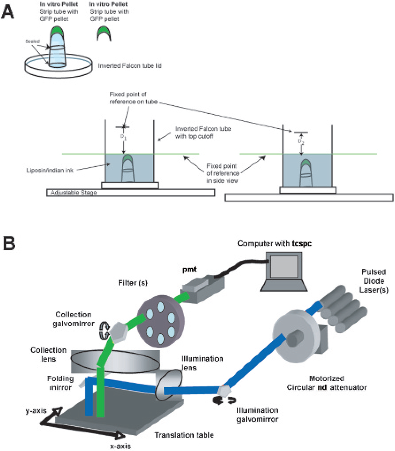
System and phantom description. A, Illustration of encapsulated green fluorescent protein (GFP) pellets used in phantom studies and actual depth determination of immersed GFP capsules in liposin–india ink solution. The phantom was placed on an adjustable stage, and liposin–india ink solution was added until the tip of the GFP capsule was just immersed. The stage was moved until the level of liposin–india ink solution was aligned with a fixed line of reference on the side-view image (green line) and a white-light image was acquired. The distance from this green line to the point of reference marked on the Falcon tube was then measured (D₁). Subsequently, more liposin–india ink was added to the phantom, and the stage was lowered so that the new level of solution again aligned with the fixed line of reference, and the new distance to the reference point on the Falcon tube was measured (D₂). D₁ – D₂ gave the depth of the GFP capsule. B, Schematic diagram of the eXplore Optix imaging system. ND = neutral density; PMT = photo-multiplier tube; TCSC = time-correlated single photon counting.

Animals

NOD/LtSz-Prkdc ^scid /B2m ^null mice (abbreviated as NOD/SCID/β2m^null, originally obtained from Dr. Leonard Schultz, Jackson Laboratories, Bar Harbor, ME) ²⁸ were expanded and maintained under defined flora conditions in individually ventilated (HEPA-filtered air) sterile microisolator cages (Techniplast, Buguggiate, Italy) at the university's animal facility. All experiments were approved by the Norwegian Animal Research Authority and conducted according to the European Convention for the Protection of Vertebrates Used for Scientific Purposes. Prior to imaging, mice were anesthetized (1% isofluorane), depilated, and moved to the heated translational stage of the eXplore Optix (ART Advanced Research Technologies Inc., Montreal, Quebec). Animals were maintained under gas anesthesia during scanning.

Capsule Implantation in Necropsied Mice

For phantom experiments with heterogeneous optical properties, mice (28–30 g) were depilated and sacrificed by CO₂ inhalation and NB4-GFP capsules were implanted subcutaneously (SC; depth = 0.3 ± 0.1 mm), intraperitoneally (IP; 0.9 ± 0.3 mm), and intramuscularly (IM; under quadriceps adjacent to the femur; 1.3 ± 0.2 mm), between the posterolateral abdominal wall and kidney (K; 1.4 ± 0.3 mm) and between the kidney and spine (S; 1.4 ± 0.2 mm), under the skull (B/IC; 2 ± 0.4 mm), and within the thorax between the lungs and ribs (T; 1.6 ± 0.3 mm). All measurements were repeated (n = 5) for capsules of 0.1, 2, 5, and 10 × 10⁶ NB4-GFP cells.

NB4-GFP Leukemia Model

NOD/SCID/β2m^null mice 6 to 8 weeks old were irradiated from a photon radiation source (BCC Dynaray CH4, 4-megavolt photon irradiation source, with a sublethal dose of 2.5 Gy [60 cGy/min]) 24 hours prior to transplantation. NB4-GFP cells (approximately 10⁷) were suspended in 200 μL of RPMI prior to injection and injected with a 28-gauge insulin needle via the dorsal tail vein. Recipient mice were monitored by weighing every second day, with imaging every seventh day following inoculation of cells, and were sacrificed following institutional guidelines when moribund, as defined by weight loss, lethargy, and/or paralysis.

Experimental Design

To investigate the linearity of the system and the effect of laser power and integration time on photon counting by the photomultiplier tube (PMT) and NB4-GFP fluorescence lifetime, an in vitro phantom of homogeneous optical properties was employed (hereafter referred to as homogeneous phantom). Capsules of 0.01, 0.1, 1, and 2 × 10⁶ NB4-GFP cells immersed in 1% liposin–50 ppm india ink solution (0.6 mm) were imaged initially with an incremental laser power of 0.125 to 4 μW at a fixed integration time (1 second) and, subsequently, with a progressive increase of integration time (0.03125 to 2 seconds) at a fixed laser power of 6 μW. Toward the development of an imageable in vivo model of NB4-GFP leukemia, validation of the sensitivity of time-domain imaging to decouple GFP fluorescence from autofluorescence and visualize NB4-GFP cells at depths and sites of expected leukemic infiltration in controlled environments was necessary. Thus, the above factors were evaluated first in an in vitro homogeneous phantom at depths of 0.6, 1.3, 2.4, 3.6, 4.7, and 6.2 mm in liposin–india ink solution. Subsequently, to evaluate if this could also be used in a mouse with heterogeneous optical properties, capsules of 0.1, 2, 5, and 10 × 10⁶ NB4-GFP cells were implanted SC, IP, and IM, K, S, B/IC, T in necropsied mice (n = 3; hereafter referred to as heterogeneous phantom). Finally, to assess disease development and establish an optical imageable model of NB4-GFP leukemia, mice (n = 9) were injected with 10⁷ NB4-GFP cells and followed longitudinally every seventh day following inoculation. Following imaging, selected mice were necropsied and tissues were excised and imaged to confirm the accuracy of the technique for early disease detection following decoupling of GFP fluorescence from autofluorescence, the depth estimate of GFP infiltrated organs, and longitudinal disease monitoring using a time-domain optical imaging approach.

Time-Domain Fluorescence Imaging

For GFP fluorescence imaging, we used an eXplore Optix time-domain imager configured (Figure 1B) for GFP imaging experiments. This consisted of a picosecond 470 nm pulsed laser diode with a repetition rate of 40 MHz (translating to an acquisition time window of 25 ns; PicoQuant, Berlin, Germany) used as a light source with a computer-controlled variable neutral density filter wheel to control laser power. After spatial filtering through a pinhole, the laser pulse is steered laterally by the illumination galvanometric mirror and redirected down on the specimen under study by a 45° folding mirror. Fluorescence emission coming from the specimen is collected through an aspheric lens. A filter bracket placed in front of the image relay allows detection wavelength selection, either of the excitation or the fluorescence wavelength, before the photons get to the PMT photocathode (Hamamatsu Photonics, Hamamatsu City, Japan). The PMT is supplied with a 12 V control voltage from the detector control board integrated in the personal computer that set the high-voltage gain on the photocathode coupled with a time-correlated single-photon counting system (Becker and Hickl, Berlin, Germany) used as a fluorescence signal detector with a 525 nm bandpass filter of 50 nm bandwidth (Omega Optical, Inc., Brattleboro, VT, and Barr Associates, Inc., Westford, MA). The laser pulse width was ≈150 ps or less. The temporal resolution of the detection system was ≈250 ps and was limited by a PMT. A translational stage and galvanometric mirrors enable raster scanning along x and y directions, with scanning resolutions of 0.5 to 3 mm possible. Samples were placed on an adjustable stage in the imaging system, where a two-dimensional scanning region and white-light image encompassing the area of the phantom or mouse were acquired via a top-reviewing digital camera. The elevation and thus the actual depth of the GFP pellets in the liposin–india ink were determined via a side-viewing digital camera with two points of reference (see Figure 1A). The samples were then automatically moved into the imaging chamber for scanning. The integration time and laser power for each sample were optimized per sample prior to scanning, except for signal linearity studies. The raster scan interval was 1 mm for phantom and in vivo studies and 0.5 mm for excised organs. Regions of interest were drawn around the position of GFP pellet inclusion (phantom studies) and scans were taken ± GFP capsules generating raw fluorescence and representative background autofluorescence data. For in vivo studies, whole-body images of leukemic mice were taken prior to leukemic inoculation and used as representative background autofluorescence, per animal.

Data Acquisition and Analysis

In time domain, ²⁹ the measured fluorescence signal is a decay curve over time F ₀ (t) where

$F_0(t)=\sum A_{i}exp(-\frac{t}{{\tau }_i})$

(1)

The decay profile is related to the lifetime of a fluorophore τ _i and other characteristics A _i , where

$A_i\propto C_i\cdot {\epsilon }_i(\lambda )\cdot L_i\cdot Q_i(\lambda )\cdot k_i\lambda \cdot S(\lambda )\cdot I_x(\lambda )$

(2)

where C _i is the molar concentration, ɛ _i (Λ) is the molar extinction coefficient, L _i is the fluorophore dimension, Q _i (Λ) is the quantum yield, k _i (Λ) is a factor related to the fluorophore excitation and emission spectrum as well as the system fluorescence filters, S(Λ) is a factor related to the instrument, for example, spectral response of the PMT, and I _x (Λ) is a spectrum of the excitation laser. Additionally, the temporal profile of the excitation laser pulse and the system impulse response function (IRF), S(t), also contribute to the signal, with the measured signal mathematically defined as the following convolution:

$F_0*S$

(3)

By comparing the data with the decay model, one can obtain the fluorescence lifetime through curve fitting, for example, least square,^30,31 maximum likelihood, or another minimization method. If a fluorophore is inside a tissue or turbid medium, there will be two more terms contributing to the convolution: the propagation of light from source to fluorophore, H(t), and the propagation of fluorescent light from fluorophore to the detector E(t), where

$H*F_0*E*S$

(4)

To precisely fit the fluorescence lifetime, all terms in the convolution need to be accounted for, making nonlinear multiparameter fitting computationally heavy. However, for fluorescence signals from small volumes of tissue such as the mouse, H(t) and E(t) do not significantly change the shape of the temporal profile of the fluorescence signal. Nevertheless, they change the peak position of fluorescence decay curve ( ^t FD_max), depending on tissue optical properties and the position of the fluorophore within tissue. Furthermore, once the excitation laser pulse and system IRF are short enough, the falling tail of the fluorescence decay curve is mainly determined by the fluorescence lifetime. It is demonstrated that as long as the full width at half-maximum of S(t) is 1.5 times longer than the fluorescence lifetime, one can get the fluorescence lifetime by only fitting the decay tail with an error less than 5% for a fluorophore in typical mouse tissues. ³² Once the fluorescence lifetime is known, it can be used to gate the intensity image. For example, if the lifetime of a fluorophore we are interested in is τ₁ and the lifetime of tissue autofluorescence is τ₂, then we can apply the following lifetime mask to the intensity image I _ij at pixel ij:

$M_{ij}=\{\begin{array}{ll}1,\hfill & if{\tau }_1-\Delta \tau <{\tau }_{ij}<{\tau }_1+\Delta \tau \hfill \\ 0,\hfill & otherwise\hfill \end{array}$

(5)

where Δτ is the lifetime fitting accuracy. If the difference of τ₁ and τ₂ is larger than Δτ, autofluorescence is eliminated in the resulting image I _ij M _ij . Data were analyzed by fluorescence lifetime decay fitting of measured signal by the Levenberg-Marquet least squares method^33,34 and fluorescence lifetime gating using Optiview software (ART Advanced Research Technologies Inc., Saint-Laurent, QC). For statistical comparison of the difference between GFP and autofluorescence ^t FD_max (Δ ^t FD_max), an unpaired Student's t-test was used, where p < .05 was considered statistically significant.

Results

Signal Linearity

Figure 2A shows a representative data set of fluorescence lifetime decays for 10⁶ NB4-GFP cells at a 0.6 mm depth, 6 μW laser power, and varied integration time (0.3125–2.0 seconds) over the 25-ns (nanosecond) acquisition window. It can be seen from this plot that fluorescence intensity doubles as integration time doubles; however, there is no change in the ^t FD_max position or slope of the fluorescence decay tail of GFP, demonstrating temporal continuity of GFP lifetime for varied integration time. Thus, the relationship of fluorescence intensity as a function of integration time per raster scan point is linear (Figure 2B). Similarly, Figure 2C shows the same number of cells and identical conditions but altering laser power (0.125–4 μW) and fixing integration time at 1 second, over the 24-second acquisition window. Again, the figures demonstrate that variation in laser power has no temporal consequence on the GFP ^t FD_max or slope of the FD, whereas Figure 2D demonstrates system linearity for fluorescence intensity with varied laser power. Consequently, all data generated can be normalized for varying laser power and integration time.

Figure 2.

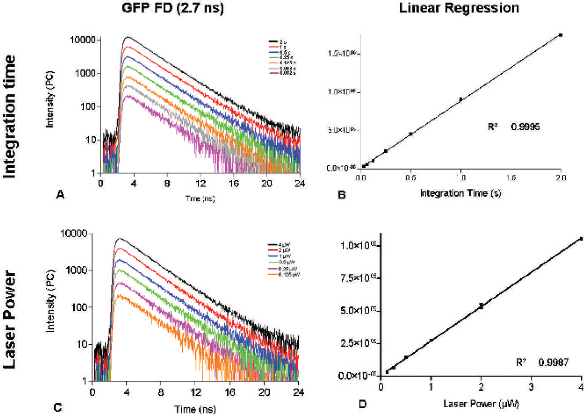
Signal linearity studies. Employing a fixed laser power of 6 μW, green fluorescent protein fluorescence decays (A) were recorded for a range of integration times (0.032–2 seconds, pink to black) with high signal linearity (R ² = .9995) for the plot of fluorescence intensity versus integration time (B). Similarly, setting a fixed integration time of 1 second and altering laser power (0.125–4 μW, black to orange) (C) resulted in exceptional linearity for the plot of fluorescence intensity versus laser power (D). Results were obtained from a fixed region of interest (20 mm²) in the homogeneous phantom described in Figure 1, using the same raster scan point per scan to generate data. Error bars represent the standard deviation of three separate measurements.

Lifetime and Depth Studies

Figure 3 illustrates the sensitivity of the time-domain imager in decoupling GFP lifetime from autofluorescence in homogeneous and heterogeneous phantoms. In the illustrated example of 2 × 10⁶ NB4-GFP cells at 4.7 mm in the homogeneous phantom (Figure 3, A-D) and 5 × 10⁶ cells under the skull in the heterogeneous phantom (Figure 3F), raw fluorescence was acquired for the field of view (FOV) ± NB4-GFP capsule. Although the fluorescence intensity of GFP capsule can just be distinguished from background in the homogeneous phantom (see Figure 3A), the background component is significant in the heterogeneous phantom, and it is difficult to determine a difference between the fluorescence lifetimes of the FOVs ± GFP capsule (see Figure 3F). By treating the data on a per pixel basis with the lifetime mask defined in equation 5, where the lifetime of GFP = 2.7 ns (unpublished observation), autofluorescence was removed and normalized GFP intensity determined (see Figure 3, C and F). Normalized GFP intensities were ascertained for capsules placed at depths of 0.6 to 6.2 mm in the homogeneous phantom (see Figure 3E) and at the various anatomic locations defined for the heterogeneous phantom (see Figure 3F). Furthermore, fluorescence decay of GFP was distinguishable from fluorescence decay of autofluorescence (see Figure 3D), and the ^t FD_max for GFP was observed to shift to later times as a function of depth when compared with the ^t FD_max of autofluorescence, which remained constant. Subsequently, normalized GFP fluorescence intensities and Δ ^t FD_max were deduced for capsules of 0.01, 0.1, and 1 × 10⁶ NB4-GFP cells in the homogeneous phantom and for capsules of 0.1, 2, 5, and 10 × 10⁶ NB4-GFP cells in the heterogeneous phantom (Figure 4).

Figure 3.

Fluorescence decoupling of green fluorescent protein (GFP) and autofluorescence for a homogeneous phantom of 2 × 10⁶ NB4-GFP cells immersed in 1% liposin containing 50 ppm india ink at depths of 0.6 to 6.2 mm (A–E) and (F) a heterogeneous phantom of 5 × 10⁶ NB4-GFP cells placed at various anatomic locations. A, Fluorescence images are obtained for GFP cells at 4.7 mm in liposin solution (raw intensity) and liposin solution only (background), and plots of their respective fluorescence lifetimes are shown in B. By subtraction of background lifetime from raw lifetime, on a pixel per pixel basis, the subtracted lifetime curve (C) of predominantly GFP versus background fluorescence lifetime is created. A clear difference in the rate of fluorescence decay and in ^t FD_max (inset C, used to estimate the depth of GFP inclusion) is observed between the GFP and background peaks. By fitting the decay tail of the measured signals (C) using the Levenberg-Marquardt least squares method, the fluorescence lifetimes are obtained. Once the fluorescence lifetime is known (GFP = 2.7 ns), it can be used to gate for GFP fluorescence lifetime only and, consequently, intensity of GFP only (D). GFP fluorescence intensity of 2 × 10⁶ NB4-GFP cells was decoupled from liposin autofluorescence at depths of 0.6 to 6.2 mm analogously. Similarly, 5 × 10⁶ NB4-GFP cells placed at various anatomic locations in a dead mouse (F) could be decoupled from autofluorescence using the mouse autofluorescence as background. Raw intensity photon counts per second (PC) are not normalized. IM = intramuscular, between the posterolateral abdominal wall and kidney (K), under the skull (B/IC), and within the thorax between the lungs and ribs (T); IP = intraperitoneal; NC = normalized counts; SC = subcutaneous.

Figure 4.

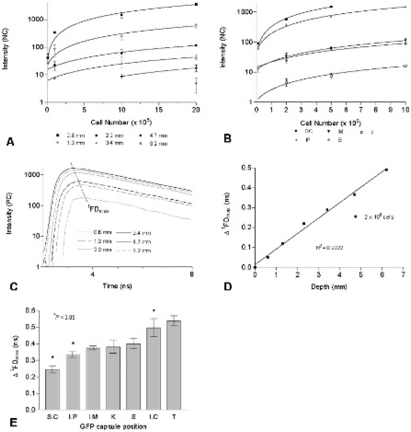
Concentration and depth and recovery for NB4–green fluorescent protein (GFP) cells in homogeneous and heterogeneous phantoms. GFP intensities for inclusions of (A) 1 × 10⁴-2 × 10⁶ NB4-GFP cells at depths of 0.6 to 6.2 mm in liposin solution and (B) 1 × 10⁴-1 × 10⁷ NB4-GFP cells placed at the defined locations in a dead mouse. C, Fluorescence decay plots of 2 × 10⁶ GFP cells at depths of 0.6 to 6.2 mm in a homogeneous phantom, with a dotted line showing shift of ^t FD_max to later times as depth increases. D, ^t FD_max shifts as a function of depth in a homogeneous phantom. E, Bar chart of shift in ^t FD_max of NB4-GFP cells at various anatomic locations in a dead mouse. Error bars indicate standard deviation of three or more data acquisitions. *p < .05.

By plotting normalized GFP fluorescence intensities for the homogeneous phantom (see Figure 4A), one can observe a linear increase in intensity with cell number (0.01, 0.1, 1 × 10⁶ NB4-GFP cells) and, conversely, a decrease in intensity as depth increases (0.6–6.2 mm). Although the same linear increase in intensity was observed in the heterogeneous phantom with increasing cell number (0.1, 2, 5, and 10 × 10⁶ NB4-GFP cells), no linear relationship was observed (see Figure 4B) in a decrease of intensity with depth, with intensity dependent on the optical characteristic of the implanted tissue. Additionally, by plotting fluorescence decay values at depths of 0.6 to 6.2 mm, a distinct shift in ^t FD_max could be observed as a function of depth (as illustrated for 2 × 10⁶ cells in Figure 4C) as the path length from source to detector increases. The relationship between Δ ^t FD_max and measured depth was linear in the homogeneous phantom (see Figure 4D). A similar relationship was noted by charting Δ ^t FD_max as a function of implantation site (SC, IP, IM, K, S, B/IC, and T) for the heterogeneous phantom (see Figure 4E). Indeed, a statistically significant difference between Δ ^t FD_max of SC and IP (p = .014), IP and combined values of IM, K, and S (as they are all of similar depths; p = .046), and, finally, B versus IM, K, and S (p = .02) was observed, suggesting that leukemic infiltrations in these tissues could be distinguished on the basis of Δ ^t FD_max.

Development of an Imageable NB4-GFP Leukemic Model

Following injection of NB4-GFP cells (10⁷) in NOD/SCID/β2m^null mice (n = 9), first detection of GFP tissue infiltrates was observed after 7 days (n = 6; Figure 5, A and C). As can be seen from the example of the mouse in Figure 5A, autofluorescence is the primary component of the overall fluorescence intensity, with autofluorescence from the stomach being the most significant feature. Despite the predominance of autofluorescence, the GFP fluorescence intensity could be decoupled from autofluorescence by treating the data on a per pixel basis with the lifetime mask defined in equation 5 in the same manner as used in the phantom studies. Comparison of the leukemic infiltrate Δ ^t FD_max (0.34) with those obtained from the heterogeneous phantom study (see Figure 4E) suggested that the infiltrate was IP. Following imaging, the mouse in Figure 5A was necropsied and the leukemic infiltrate of the ureter was excised (see inset, Figure 5A). Similarly, by imaging mice with the time-domain imager, leukemic development was followed on a weekly basis to week 3 in a second mouse (see Figure 5B). Following imaging and determination of Δ ^t FD_max for selected infiltrates (see table, Figure 5B), the mouse was necropsied and leukemic organs excised. All excised leukemic infiltrates observed from imaging were found in the anatomic compartments suggested by the Δ ^t FD_max calculated from the in vivo image (see Figure 5B). Leukemic infiltration of the bone marrow (femur), ureter, kidney, and central nervous system and extensive infiltration of the lymph nodes could be determined and their approximate anatomic location estimated from Δ ^t FD_max values. Subsequently, the remaining mice (n = 6) were monitored for leukemic development longitudinally by time-domain imaging (n = 4 developed leukemia, example of one mouse in Figure 5C). Definitive disease confirmation could be determined only from raw fluorescence intensity by week 3, with leukemic animals succumbing to disease by week 4. By decoupling GFP fluorescence intensity from raw fluorescence intensity and thus autofluorescence, leukemic infiltrates were detected by week 1, with an initially slowly developing phenotype progressing to aggressive disease from week 3.

Figure 5.

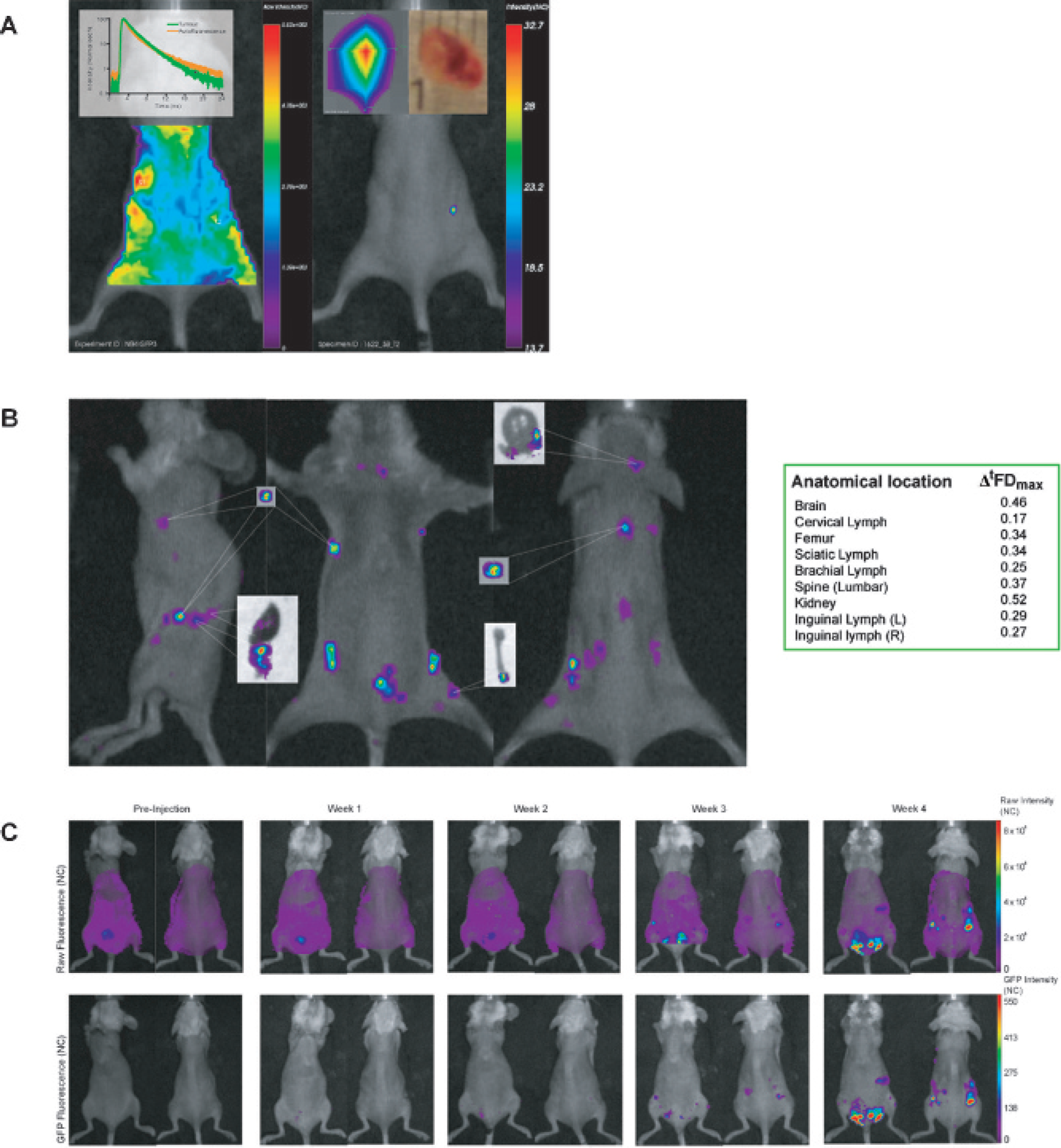
NB4–green fluorescent protein (GFP) in vivo AML model. A, Raw fluorescence intensity image acquired 7 days after inoculation of 1 × 10⁷ NB4-GFP cells and subsequent gated image for GFP fluorescence lifetime. Insets show a plot of autofluorescence lifetime versus GFP fluorescence lifetime for the tumor shown. B, GFP fluorescence lifetime gated images for a mouse with extensive leukemia infiltrates (28 days following injection with 1 × 10⁷ NB4-GFP cells) and selected excised organs. The table exhibits the Δ ^t FD_max for the NB4-GFP leukemic infiltrates, aiding distinction between the different GFP infiltrates. C, Longitudinal imaging of the NB4-GFP leukemia model in vivo. The top panel exhibits the raw fluorescence intensity images from preinjection to week 4. It is possible to definitively distinguish GFP infiltrates from raw fluorescence only after 3 weeks. The bottom panel shows the GFP fluorescence lifetime gated images of the corresponding raw fluorescence intensity images. Using this method, GFP infiltration of the knee and lymph nodes can be detected as early as 1 week following inoculation, and further infiltration of spleen, ovaries, kidney, and extensive lymph can be followed longitudinally.

Discussion

We generated a GFP⁺ human promyelocytic leukemia cell line, NB4, and subsequently developed an NB4-GFP human xenograft leukemia model in NOD/SCID/β2m^null mice. As imaging of GFP is frustrated by complications in the visible spectrum, primarily by spectrally similar endogenous autofluorescence emission, we sought to validate the sensitivity of time-domain imaging to decouple GFP fluorescence from autofluorescence; to visualize NB4-GFP cells at depths and sites of expected leukemic infiltration in controlled phantom environments; and finally to assess disease development in an optical imageable model of NB4-GFP leukemia.

Time-domain measurements and subsequent decoupling of raw fluorescence are dependent on fluorescence lifetime. Additionally, increasing fluorescence intensities in vivo as GFP fluorescence increases requires the use of various laser powers and integration times for optimized imaging of a region of interest over the course of disease. Thus, it was important to establish that deviation of these parameters has no effect on the resultant fluorescence lifetime and that variation in laser power and/or integration time could be normalized, enabling direct result comparison. As can be seen from Figure 2, variation of laser power and integration time had no effect on the position of ^t FD_max or the rate of decay of the fluorescence decays. Furthermore, changes could be normalized linearly, permitting direct comparison of results obtained with diverse laser powers and integration times. Having first established the signal linearity of the system for laser power and integration time, we then assessed the ability of the imager to decouple GFP fluorescence from autofluorescence and visualized NB4-GFP cells at depths and sites of expected leukemic infiltration in controlled phantom environments.

Employing a phantom of homogeneous optical properties, consisting of capsules of defined NB4-GFP cell number (0.01–2 × 10⁶ cells) immersed in liposin–india ink solution, it was demonstrated that by applying a lifetime mask, defined in equation 5, on a per pixel basis, autofluorescence is removed and normalized GFP intensity is determined from raw fluorescence (see Figure 3, C and F). By plotting normalized GFP fluorescence intensities against cell number, a linear increase in intensity was observed with increasing cell number and a subsequent decrease with increasing depth (see Figure 4A). Furthermore, following decoupling of GFP fluorescence intensity from background autofluorescence, a distinct shift in GFP ^t FD_max was observed in comparison with corresponding background ^t FD_max (see Figure 3C), which increased with deepening depth of the GFP capsule in the phantom (see Figure 4C). By plotting Δ ^t FD_max as a function of depth, a linear relationship could be determined (see Figure 4D). Thus, the results from the homogeneous phantom suggested that if the depth of GFP inclusion could be determined from Δ ^t FD_max, one could then estimate cell number by extrapolation of Figure 4A in a homogeneous phantom. To investigate whether this thesis held in a phantom of similar heterogeneous optical properties as live mouse, cell pellets were implanted in necropsied mice at defined anatomic locations of varying depths and tissue compartments. Normalized GFP intensities and Δ ^t FD_max were determined and plotted, as above (Figure 4, B and E). Although a linear increase in normalized GFP intensity could be observed with increasing cell number per tissue compartment, no correlation of GFP intensity could be made as a function of depth (see Figure 4B). Instead, it appeared that the detected level of GFP intensity of the implanted capsules was dependent on the optical properties of the tissue compartment they were implanted in. However, similar to Figure 4D, changes in Δ ^t FD_max appeared to be independent of the tissue properties of capsule implantation site reflecting instead the depth of the implant in the phantom sites examined. Indeed, statistically significant differences could be demonstrated between Δ ^t FD_max of SC and IP; IP and the combined values for IM, K, and S (which were all of similar depth by caliper measurement); and B versus IM, K, and S, suggesting that if similar Δ ^t FD_max were observed in vivo, the results from this phantom model could be used to determine the tissue of origin for NB4-GFP tissue infiltrates.

Subsequent to these phantom studies, NOD/SCID/β2m^null mice (n = 9) were injected intravenously with 10⁷ NB4-GFP cells. Although a primary aim of this study was to determine if NB4-GFP could be followed longitudinally in vivo to develop an imageable model of AML, we first had to confirm that the lifetime gating mask employed in the phantom studies also applied in vivo. Thus, following imaging 7 days after cell inoculation, initial detection of GFP fluorescence was observed (n = 6). In the example shown in Figure 5A, comparison of Δ ^t FD_max with values obtained from the heterogeneous phantom study (see Figure 4E) suggested that the leukemic infiltrate was IP. Following necropsy, the tumor was located in the ureter within the IP cavity, suggesting that the values obtained from the phantom studies could be used to determine the tissue of origin for comparable infiltrates in vivo. Development of leukemia in a second mouse was monitored longitudinally by time-domain imaging to compare multiple GFP infiltrates in various sites with corresponding phantom values, and following imaging, the mouse was necropsied. This animal was particularly interesting as several tumors, particularly on the lower left dorsal aspect of the mouse (see the lateral view in Figure 5B), exhibited different Δ ^t FD_max (0.52–0.29), even though they appeared from planar time-domain imaging to be located in a similar anatomic location. Resection of GFP-infiltrated organs revealed that although leukemic infiltrates were located in a similar two-dimensional spatial location, they were, indeed, located at different depths (inguinal lymph, tumor of the ureter and kidney; see insets in Figure 5B). Additionally, leukemic tumors in the brain, central nervous system, and femur and extensive lymph node infiltration were discerned from autofluorescence by time-domain imaging and approximate depth was estimated by Δ ^t FD_max and confirmed by necropsy.

The remaining mice (n = 6; one mouse died 3 days following irradiation) were monitored longitudinally by imaging until they became moribund (n = 4; example of one mouse in Figure 5C), when they were humanely sacrificed, or if after 4 weeks of monitoring by imaging no GFP fluorescence was observed (n = 2), imaging was stopped, animals were monitored daily, and weights were taken twice per week. Neither of these animals died from leukemia. Six of eight mice developed leukemia, five of which exhibited similar disease pathogenesis, as observed for the example in Figure 5C, characterized by initial infiltration of the femoral bone marrow and superficial lymph nodes (day 7) and slow disease progression up to days 14 to 21, when exponential leukemic growth was observed as monitored by time-domain fluorescence imaging, with animals becoming moribund soon after.

We conclude that early disease detection through use of time-domain imaging in this initially slowly progressing AML xenograft model permits accurate disease staging and should aid in future preclinical development of therapeutics for AML.