ntPET: A New Application of PET Imaging for Characterizing the Kinetics of Endogenous Neurotransmitter Release

Abstract

We present a new application of positron emission tomography (“ntPET” or “neurotransmitter PET”) designed to recover temporal patterns of neurotransmitter release from dynamic data. Our approach employs an enhanced tracer kinetic model that describes uptake of a labeled dopamine D2/D3 receptor ligand in the presence of a time-varying rise and fall in endogenous dopamine. Data must be acquired during both baseline and stimulus (transient dopamine release) conditions. Data from a reference region in both conditions are used as an input function, which alleviates the need for any arterial blood sampling. We use simulation studies to demonstrate the ability of the method to recover the temporal characteristics of an increase in dopamine concentration that might be expected following a drug treatment. The accuracy and precision of the method—as well as its potential for false-positive responses due to noise or changes in blood flow—were examined. Finally, we applied the ntPET method to small-animal imaging data in order to produce the first noninvasive assay of the time-varying release of dopamine in the rat striatum following alcohol.

Introduction

The utility of positron emission tomography (PET) for detecting net changes in endogenous neurotransmitters after a stimulus has already been demonstrated through a variety of approaches [1–9]. However, most studies have asked a simple binary question: Did neurotransmitter levels increase or decrease? Our present focus is not merely on the detection of increases in neurotransmitter, but also on the characterization of the temporal signature of a neurotransmitter's response to stimuli. We believe that development of neurochemical assays that capture these temporal signatures is critical because the dynamics of synaptic neurotransmitter concentrations have been invoked to explain the addictiveness of drugs [10] and, more generally, neurotransmitter dynamics may encode both normal and abnormal cognitive or behavioral functions. The elucidation of specific patterns of neurotransmitter fluctuation would, thus, be beneficial to the study of a wide range of neuropsychiatric diseases, including alcohol and substance abuse disorders.

The purpose of this article is to describe and demonstrate the feasibility of a new technique for visualizing time-varying neurotransmitter concentrations via PET (“ntPET,” i.e., “neurotransmitter PET”). This new method relies on an enhancement of the standard tracer kinetic model typically applied to PET data. The enhanced model we propose accounts for both the time-varying dynamics of the radiotracer that we employ, [¹¹C]raclopride ([¹¹C]RAC, a dopamine D2/D3 receptor antagonist), and the endogenous neurotransmitter dopamine (DA) that competes with it. To make the technique practical in small animals, the model has been developed using a reference region approach. There is no need for arterial sampling of the input function in this method. Experimentally, the data must be acquired in two separate PET scans: one conducted with the animal at rest (“baseline” condition), the other immediately following a stimulus that induces a transient increase in striatal DA concentration (aka, “activation” or “stimulus” condition). In this article, we demonstrate the accuracy and sensitivity of the method by analyzing realistic simulation studies. We also begin to address the precision and biological validity of the method by analyzing preliminary data acquired in rats receiving alcohol (to cause release of DA) and in rats imaged during control conditions.

What Developments and Observations have Prompted us to Develop a New Imaging Method?

The rewarding effects of pleasurable stimuli are driven, in part, by the dopaminergic projection from the ventral tegmental area to the nucleus accumbens (“the mesolimbic DA system”). DA is thought to play a critical role in mediating the reinforcing properties of rewarding stimuli [11–15]. Alcohol and other drugs of abuse (e.g., cocaine, methamphetamine) cause increases in DA concentration in the striatum, which contains the nucleus accumbens. It has been hypothesized that the rewarding properties and addictive liabilities of drugs of abuse may be related to the kinetics of DA elevation [16,17]. It has been shown with [¹¹C]methylphenidate PET imaging that intravenous methylphenidate reaches the brain much faster than an oral dose. The ability of the intravenous drug to increase DA concentration rapidly almost certainly underlies its euphoric effect. In their review of methylphenidate abuse, Volkow and Swanson [10] went so far as to state, “the relevant variable for [the study of] reinforcement is the magnitude of the dopamine change per time unit.” We see the development of ntPET as a means to explore directly, and in detail, the process of DA elevation (and any alterations therein) and its possible role in substance abuse disorders such as alcohol abuse. Several studies have already documented that alcohol releases DA in the striatum of rodents [18–27]. However, these studies provide only crude descriptions of the temporal patterns resulting from DA release because of limitations in the temporal resolution of the experimental techniques employed.

What is the State of Current Tools for Probing Temporal Changes in DA?

In vivo microdialysis and voltammetry are the two established methods commonly used to assess stimulus-induced changes in DA concentration. Each technique suffers inherent limitations that are circumvented by ntPET. Microdialysis and voltammetry require intracranial cannulation, which precludes within-animal longitudinal studies. Additionally, microdialysis and voltammetry measure changes in extracellular neurotransmitter concentrations, which may not directly correspond to events that occur within the synapse, the milieu of neurotransmission. The DA curves estimated via ntPET reflect events that are occurring intrasynaptically; specifically, we measure the time-varying competitive displacement of bound [¹¹C]RAC from postsynaptic D2/D3 receptors by increases in endogenous DA [28,29]. We cannot measure from individual synapses, of course, but we can visualize the ensemble pattern of activation of the DA system in brain regions. Another good reason to develop a PET-based tool for intrasynaptic neurotransmitter measurement is that the same tool that we develop for small animals can be applied to humans (probably with greater success because the higher signal-to-noise data possible from human imaging will lead to better performance of ntPET.)

How Does One Make Kinetic Measurements of Endogenous Neurotransmitters?

To recover meaningful parameters that describe physiological processes from PET data, the data must be fit with a compartmental model that describes the uptake and retention of target-specific radiotracers by a tissue of interest. The model must account for the kinetic “states” of a tracer in the tissue, and the fluxes between states. The earliest PET models [30] neglected endogenous neurotransmitters and were based on the premise that, if present, the concentrations of any endogenous ligands were constant throughout the scanning period. A useful compound parameter to emerge from early models was the binding potential (BP) (equal to the steady-state ratio of bound to free tracer). BP has found use as a stand-in for number of receptors, B^max, which is harder to measure. BP can also be used for in vivo neurotransmitter assays.

Apparent changes in BP after some treatment are regularly attributed to changes in the level of the neurotransmitter that competes with the tracer [5–8]. Unfortunately, with a single index, it is not possible to represent complex information related to both timing and magnitude. In fact, changes in the former can sometimes be confused for changes in the latter [31]. The questions we want to ask are: Did the DA concentration increase quickly? Precisely when did it peak? How high was the peak relative to the baseline? To answer these questions, we must formulate a more comprehensive model.

Materials and Methods

Kinetic Model Development

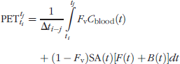
Figure 1A represents an extension of the standard PET model to account for time variations in endogenous ligand concentration [32]. It includes compartments for tracer as well as endogenous species (DA). The balance on the free tracer, F, is

$\begin{array}{c}\frac{dF(t)}{dt}=K_1{C}_p(t)-k_{2}F(t)\\ -k_{\text{on}}\left[B_{max}-B(t)-B^{\text{DA}}(t)\right]F(t)\end{array}$

1

Figure 1.

(A) The enhanced model corresponding to Equations 1–3. Plasma (C_p), free (F), and bound (B) refer to tracer. Free (F^DA) and bound (B^DA) refer to endogenous ligand. The dotted rectangle around the two bound compartments refers to the competition between B and B_DA for a limited number of receptors. (B) If plasma data (C_p) are not available, data from a REF region (and its derivative in time) can be used instead as the input function to the model.

The rate constants have the same interpretation as in the standard two-tissue compartment model used frequently in PET. C^p(t) is the plasma concentration of tracer. Normally, this quantity must be measured directly via arterial blood sampling. The balance on the bound tracer, B, is

$\frac{dB(t)}{dt}=k_{\text{on}}\left[B_{max}-B(t)-B^{\text{DA}}(t)\right]F(t)-k_{\text{off}}B(t)$

2

F and B have the standard definitions: Free and bound molar concentrations (pmol/mL), respectively.

The addition to the standard model consists of the free DA, F^DA, and the bound DA, B^DA. The balance on the bound endogenous DA is

$\begin{array}{c}\frac{d{B}^{DA}(t)}{dt}=k_{\text{on}}^{\text{DA}}\left[B_{max}-B(t)-B^{\text{DA}}(t)\right]F^{\text{DA}}(t)\\ -k_{\text{off}}^{\text{DA}}{B}^{\text{DA}}(t)\end{array}$

3

where k^DA_on and k^DA_off are the association and dissociation rate constants, respectively, for endogenous DA at the D2/D3 receptor site. F^DA(t) can be treated as an additional input to the system. Equation 3 is coupled to the standard model (Equations 1 and 2) through the specific binding term (B_max–B–B^DA)F^DA. This term shows that binding is bimolecular and saturable. Specific binding of tracer (Equation 2) depends on concentration of available receptors (B_max–B–B^DA) and on free tracer, F. In the enhanced model (Equations 1–3), B_max must refer to the concentration of all the D2/D3 receptors (contrast this with the parameter that occurs in the standard model, B′_max, defined as all available D2/D3 receptors at steady state) [33].

Using a Reference Region as an Input. As stated above, C_p(t), can be measured from arterial samples. It is possible to avoid this procedure, provided there are regions of the image that can serve as a “reference” region [34,35]. Figure 1B represents a reference region (REF), which is defined as an area that lacks the receptors that bind the radioligand. We will use data from a REF to alleviate the need for an arterial curve. To use a REF approach, we adopt an alternative formulation of the basic kinetic model [34]. Specifically, Equation 1 (with binding constant, k_on = 0) can be rearranged to yield an expression for the plasma in terms of the free tracer in a REF, F^Ref(t):

$C_{\mathrm{p}}(t)=\frac{1}{K_1^{\text{Ref}}}\left[\frac{d{F}^{\text{Ref}}(t)}{dt}+k_2^{\text{Ref}}{F}^{\text{Ref}}(t)\right]$

4

As long as the PET signal in the REF is a good approximation to the contents of its free compartment (which is valid except early in the scan, immediately following the injection of tracer), the model can be reformulated by incorporating Equation 4 into the standard model (Equation 1) to eliminate C_p(t). In our implementation of the REF approach, we spline the true activity curve (TAC) from the cerebellum (via “pchip,” a shape-preserving cubic spline function in Matlab, The Mathworks, Natick, MA); use that splined curve as our measured F^Ref(t) and differentiate the splined curve to get the derivative required in Equation 4.

A Function to Model Time-Varying Dopamine. A transient increase in DA release induced by a stimulus constitutes an unknown—and not directly observable—input to the system. Estimating the pattern of this transient release over time, F^DA(t), is our primary goal. In vivo studies of drug-induced increases in mesolimbic DA suggest that DA typically rises and falls unimodally in response to alcohol [18–23,26,36] or other experimental stimuli [37–41]. Therefore, we choose to parameterize the unknown input as a gamma variate with an offset (Basal), leading coefficient (G), and delay (aka, takeoff, t_D). We describe the stimulus-induced increase in intrasynaptic DA in terms of the five parameters of the gamma variate function, Θ_DA = [Basal, G, t_D, α, β]^T, as:

$F^{\text{DA}}(t)=\text{Basal}+G^{*}{\left[t-t_{\mathrm{D}}\right]}^{\alpha }exp\left(-\beta \left[t-t_{\mathrm{D}}\right]\right).$

5

The peak height of F^DA occurs at a peak time, t = t_D + α/β.

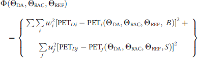
PET Output Equation. Although the enhanced model contains terms for an endogenous species, the expression for the discrete PET output is unchanged from standard models. It is the weighted sum of radioactivity concentrations in tissue compartments and in whole blood, integrated over the frame time:

$\begin{array}{c}{\text{PET}}_{t_i}^{t_j}=\frac{1}{\Delta t_{i-j}}\underset{t_i}{\overset{t_j}{\int }}{F}_v{C}_{\text{blood}}(t)\\ +\left(1+F_v\right)SA(t)\left[F(t)+B(t)\right]dt\end{array}$

6

Exponentially decaying specific activity, SA(t), converts molar quantities of F and B to radioactivity. The weightings are based on the respective volume fractions. F_v is the blood volume fraction of the region of interest (ROI). C_blood(t) is the whole blood radioactivity concentration.

Simulations

Activation Condition. For each case to be examined, we created 10 realistic simulations of TACs in the striatum at baseline and 10 during the stimulus condition by solving the model shown in Figure 1A (Equations 1–3, 5, 6). A single arterial input, C_p(t), was simulated for both conditions based on real [¹¹C]RAC data in rats. To test the REF approach to the estimation of stimulus-induced DA curves requires reference region TACs. Specifically, we created 10 cerebellum curves for both conditions. Hence, a simulation dataset consisted of two striatum curves and two cerebellum curves for each case that was addressed. Blood flow parameters (K₁, k₂) used for a given striatal curve were also used for the associated cerebellar curve, except in the specific case where change in K₁ was being examined (see below). For every simulation set to be created, tracer parameters, Θ_RAC (= [K₁, k₂, k_on, k_off, B_max]^T), were selected randomly from a uniform distribution (±10%) around canonical parameter values based on our [¹¹C]RAC scan data in rats. k^DA_on and k^DA_off were fixed at large values that were compatible with the measured affinity constant for DA at the D2/D3 receptor (K_D = 100 nM; [42]). The same DA curve parameters, Θ_DA, were used for every stimulus condition simulated. Varying tracer parameters for each simulation set is akin to simulating inter-rat variability in the uptake and retention of raclopride. All baseline simulations were created with DA fixed at the same Basal concentration (100 nM) so occupancy of D2/D3 by DA was 50% at baseline. Constant DA level at baseline is an assumption of our model (see Parameter Estimation), and with regard to this point, our simulated data were always in compliance. The DA curve used in all the stimulus conditions was derived from actual [¹¹C]cocaine PET data [43] in order to approximate the DA response that might occur following administration of a moderate dose of intravenous cocaine (for details, please see Ref. [31]). By way of comparison with other studies, the average ΔBP by graphical analysis [44] for the 10 simulated PET datasets containing a nonconstant DA curve was 0.28 ± 0.11. Noise was added [45] to produce the noise level observed in our animal experiments. All models were implemented in Matlab using COMKAT [46].

Control (Null) Condition. We simulated an additional 98 datasets that paired two baseline striatal TACs (and the accompanying cerebellar TACs) that differed only in their particular noise realizations. To address the likelihood and magnitude of false positives, these data were then analyzed with the complete “ntPET” method as if one of the two had been acquired during an activation condition. The mean BP for 196 null cases (98 “rest” plus 98 “activation”) was 1.012 ± 0.138 and the mean ΔBP was 0.033 ± 0.095, confirming that the null data were configured with no detectable DA change.

Null Condition with K₁ Decrease. To investigate the possibility that change in some aspect of tracer uptake other than competition with DA could masquerade as a DA change, we created additional null simulations that included a 25% reduction in K₁ relative to baseline for the duration of the “activation” scan. An increase in blood flow is unlikely to be confused with a DA increase as more blood flow would cause higher tracer uptake, whereas DA competition will cause a decrease in PET signal. Of course, logically, a decrease in blood flow should affect both K₁ and k₂, but it has already been shown that a concomitant change in both parameters does not appreciably alter the PET signal [3,4]. We examined a drop in K₁ alone to probe for extreme (and probably unphysiologic) perturbations that might cause pronounced false-positive results [4]; examining an increase in k₂ alone would produce comparable results because increasing efflux and decreasing influx both lower net uptake.

Small-Animal Imaging Protocol

Three high-alcohol drinking (HAD) [47] rats (423 ± 28 g) each received two [¹¹C]RAC PET scans on different days. Before each scan, rats were anesthetized with an intramuscular injection of 0.1 mL per 100 g body weight ketamine cocktail (ketamine/xylazine) 20 min before the tracer. Two “alcohol” animals received a scan at baseline, and another scan some time after an intraperitoneal alcohol challenge. Rat A received 0.5 g/kg 11 min prior to injection of [¹¹C]RAC; Rat B received 1.5 g/kg of alcohol intraperitoneally 2.5 hr prior to injection of [¹¹C]RAC. The control animal (Rat C) received two baseline scans.

Animals were gently secured on the scanner bed in the supine position. At scan start, 0.326 ± 0.109 mCi [¹¹C]RAC was injected through the tail vein; scans lasted 60 min. The injected SA was 0.355 ± 0.185 Ci/mmol and mass dose of raclopride for all scans was 3.34 ± 3.57 nmol/kg. Images were reconstructed (filtered back-projection) using the following time frames: 6 × 60, 2 × 120, 4 × 150, 8 × 300 sec. The spatial resolution of the IndyPET II is 2.5 mm FWHM at the center of the field of view; axial resolution is 4.1 mm FWHM [48].

Circular ROIs (11 voxels ^*0.625 ^* 0.625 ^* 3.15 = 13.54 mm³) were positioned on the left and right striatum on a single slice and on the cerebellum (57.83 mm³), also on a single axial slice. Left and right striatal values were averaged. ROI placement and the resulting typical cerebellum and (pooled) striatum TACs for the case of a baseline condition scan are illustrated in Figure 2.

Figure 2.

(A, B) MIP images show axial positions of the striatum and cerebellum, respectively. (C, D) Striatal and cerebellar slices of [¹¹C]RAC images with circular ROIs positioned on the left and right striatum (C) and cerebellum (D). (E) Typical striatal and cerebellar TACs. Striatal curve is based on pooled left and right striatal ROI data. Note separation of curves indicating detection of considerable specific (displaceable) binding of [¹¹C]RAC.

Parameter Estimation

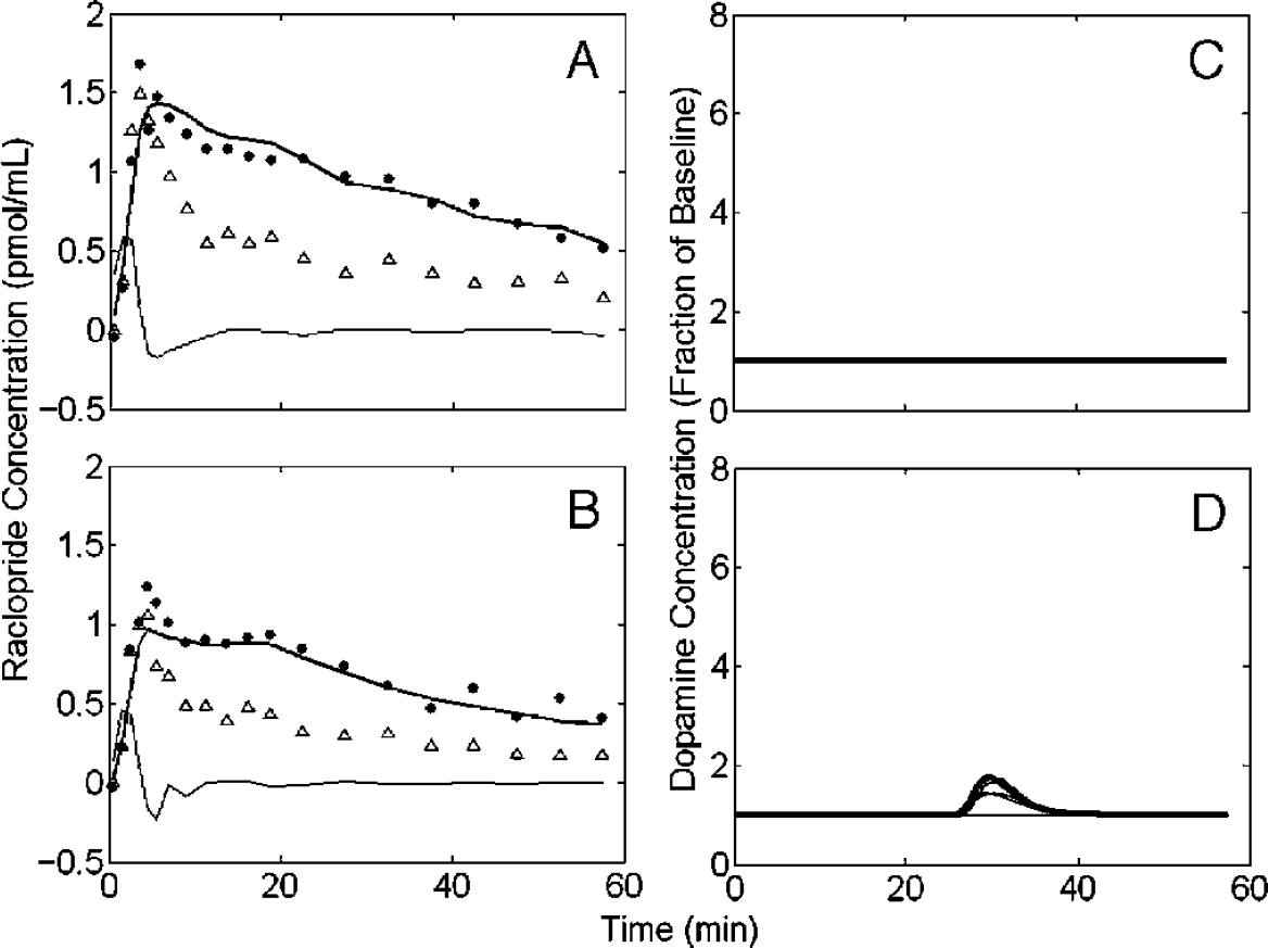
The power of our method to estimate new information from dynamic PET comes from fitting our model to data from rest and stimulus conditions simultaneously (a “concatenated dataset”). In doing so, we assume that the tracer parameters remain constant across conditions and the DA curve is allowed to vary only in the stimulus condition. This is not unlike modeling approaches that have sought to improve parameter identifiability by simultaneously fitting data acquired either from multiple regions or at multiple SAs [49–54]. The best fit to the concatenated dataset (baseline plus stimulus conditions) is found by minimizing the objective function, Φ, over the space of all parameters (Θ_DA, Θ_RAC, Θ_REF). (The REF formulation introduces two new parameters [R_i = K₁/K₁^ref and k₂′ = Rⁱk₂^ref] but only one net additional parameter as it eliminates K₁ from Θ_RAC). The compound objective function is the weighted sum of squared residuals (WSSR) over both baseline (B) and stimulus (S) conditions:

$\begin{array}{l}Ф\left({\Theta }_{\text{DA}},{\Theta }_{\text{RAC}},{\Theta }_{\text{REF}}\right)\hfill \\ =\left\{\begin{array}{l}\sum \sum _i{w}_i^2{\left[{\text{PET}}_{Di}-{\text{PET}}_i\left({\Theta }_{\text{DA}},{\Theta }_{\text{RAC}},{\Theta }_{\text{REF}},B\right)\right]}^2+\hfill \\ \sum _j{u}_j^2{\left[{\text{PET}}_{Dj}-{\text{PET}}_j\left({\Theta }_{\text{DA}},{\Theta }_{\text{RAC}},{\Theta }_{\text{REF}},S\right)\right]}^2\hfill \end{array}\right\}\hfill \end{array}$

7

PET _Dx is the xth data point in a given condition. PET _x is the solution to the model (Equations 1–6) at the same point; w² _i and u² _j weight each residual inversely according to its variance. The precision of the estimates can be improved by the addition of “prior” information to the objective function via one or more penalty functions [55]. An example is given in Equation 8:

$\begin{array}{l}Ф{\left({\Theta }_{\text{DA}},{\Theta }_{\text{RAC}},{\Theta }_{\text{REF}}\right)}_{\text{penalized}}\hfill \\ =\left\{\begin{array}{l}Ф\left({\Theta }_{\text{DA}},{\Theta }_{\text{RAC}},{\Theta }_{\text{REF}}\right)+\hfill \\ \tau \left({\text{BP}}_{\text{graphical}}-\text{BP}\left({\Theta }_{\text{DA}},{\Theta }_{\text{RAC}},{\Theta }_{\text{REF}}\right)\right)\hfill \end{array}\right\}\hfill \end{array}$

8

In this case, a penalty term has been appended to the objective function, Φ, that requires independent knowledge of BP. Minimizing the penalized objective function thus favors a choice of parameters that yields a BP that is “close” to the known value of BP—in our case, a value that is measured concurrently but by an independent means [44]—from the baseline data. “Close” depends on the choice of weight for the penalty function, τ. We chose the weight of the penalty term according to a preliminary optimization that sought to minimize the variances in the estimates of DA peak time, peak height, and takeoff, from simulated data. Based on such an analysis, τ was set to 60 and was large enough to force the estimated BP—a macroparameter made up of a number of model parameters—to converge to roughly its measured value. Despite limitations, described above, one might also imagine using some applicable aspect of microdialysis data (e.g., the normalized area under the measured DA curve) from appropriately treated rats, as another type of prior information to help guide the minimization of a penalized objective function. In this way, one could search for DA curves that satisfy the PET data and yet are not inconsistent with a trove of existing data from another experimental method.

The quality of our experimental data supported the estimation of three tracer (k₂, k_on, k_off), two REF (R_i and k₂′), and five DA parameters (Θ_DA) simultaneously. For all fits, the binding rate constants for DA were fixed to fast values (k^DA_on = 0.25 mL/(pmol min); k^DA_off = 25 min⁻¹) based on an earlier review of the literature [42]. The parameters Basal and B_max were not strictly identifiable, so B_max needed to be fixed during fitting. When fitting simulated data, we wanted to perform a fair test of our estimation method, so we were careful to fix B_max to something other than the true value. We chose to fix it at a reasonable value (50 nM) based on the literature and on initial fits to rat data (for which we allowed all Θ_DA parameters to vary). Recall that simulations were created with Θ_RAC parameters varying by ±10% around a mean. The true B_max varied in the range 36–44 nM]. Because we are only interested in positive changes in DA, we restricted G to values equal to or greater than zero. Hence, F^DA(t) curves were restricted to positive values at or above baseline. Choices for all other estimated parameters were limited above and below by loose upper and lower bounds [e.g., 0.01 ≤ k_on ≤ 1 mL/(pmol min)].

Best-Fit Criteria. Even with the use of data from two conditions, the task of fitting our enhanced model and 10 parameters to the data is an ill-posed problem. Hence, we are not surprised to find some dependence of fitted values on initial parameter guesses. In general, this is due to two factors: inherent correlation between some parameters which creates multiple combinations of equivalent parameter groupings, and noise in the data which creates local minima in the functions Φ or Φ_penalized. To overcome the dependence on initial guess, two additional steps were taken. (1) Fits of each dataset were always performed starting from 100 different initial parameter guesses. The initial guesses varied widely and randomly. (2) Of the fits that converged, the retained results consist of those fits that met our two-stage best-fit criteria: (i) WSSR lower than the median WSSR and (ii) of the results retained in Step 1, the number of runs (i.e., zero-crossings in the residuals [56]) had to be greater than the median number of runs. It is worth noting that taking this “Monte Carlo” approach to estimation leads us to present multiple best DA curves for every dataset.

Testing the Method

Our initial tests of ntPET were performed in six steps. (i) A series of realistic simulations that closely resembled our dynamic rat data were analyzed to determine whether we could recover the true DA input that produced the simulated data—and with what accuracy and precision. (ii) At the same time, we analyzed simulated datasets that represented “null” cases to test for Type I errors. That is, what DA curve(s) is recovered by our method when the only differences between the baseline and activated data are due to random noise? These simulations were used to determine a detectability threshold. To achieve a false-positive rate of zero, a detectability threshold must be set to exclude any DA curves that might be generated by noise alone. Because it may not be possible to achieve perfection with our data, we selected a detectability threshold that yielded only one false-positive event in 10 “null” datasets. (iii) Third, we tested for additional false-positive DA curves in “null” case simulations that also included a manufactured artifact related to change in blood flow during activation. To test the worst-case scenario, we created data whose K₁ value (only) was depressed by 25% in the activated case. There was no true DA change included in these simulations. The question we asked was: Can noise and an extreme blood flow artifact yield a DA curve that looks like our findings in animals? (iv) The DA response was recovered from rat data acquired immediately following intraperitoneal alcohol; the precision of the parameter estimates was determined and the overall findings were compared with published results based on microdialysis experiments. (v) To address concerns in the literature about prolonged effects of drugs on number of D2/D3 receptors (aka, “receptor internalization”), we scanned a rat at baseline and 2.5 hr following intraperitoneal alcohol. (vi) Finally, ntPET was applied to rat control data which were acquired in two scans without any real stimulus during either scan to see whether experimental variations of any sort between scans could mimic a real DA response.

Results

Simulations of Activation

Figure 3 shows a typical result of fitting the model described in Equations 1–6 to one simulated noisy concatenated dataset created with time-varying endogenous DA. Figure 3A and B constitutes a representative fit of the model to a simulation of the striatal region in the baseline (Figure 3A) and stimulus (Figure 3B) conditions. The simulated cerebellum data (lower curves in Figure 3A and B) are also plotted for each condition. The plasma curves used to simulate the data via the model in Figure 1A are also shown on each of the left-hand panels as dashed curves. During estimation, the measured cerebellum data are not fitted explicitly but are used as a measure of F^ref(t) and its time derivative (Equation 6) to substitute for a directly measured arterial input function. The derivative of the splined cerebellum curve is shown in Figure 3A and B because its quality dictates, in part, the quality of the input. Figure 3C simply illustrates the assumption of the enhanced model that DA does not change during the baseline condition. Figure 3D displays the resulting “best” DA curves, selected according the to best-fit criteria, recovered by minimizing Equation 8 over most model parameters (B_max, k^DA_on, and k^DA_off are fixed) for the simulated dataset shown on the left-hand side of the figure. The true DA curve takeoff time, peak time, and peak height are indicated by arrows (true values: takeoff = 8 min; peak time = 16.26 min; peak height = 5.132 × baseline DA). Note that the scale of the recovered DA curves is in fraction of baseline.

Figure 3.

Simulated rat data from striatum (filled circles) and cerebellum (triangles) in the rest (A) and activated states (B). The data were simulated using the plasma input curves (dashed curves, scaled) and the model in Figure 1A. The smooth curve through the striatal points is a fit of the REF model (given in Figure 1A and B) to all the data in A and B simultaneously. The thin solid curves in A and B are the time derivatives of the cerebellum curves; these are used by the REF model in lieu of a plasma curve. (C) The model assumption that DA is quiescent at rest is demonstrated. (D) The black curves are the resulting DA curves from best fits to the data in A and B. The true DA takeoff and peak times are indicated by vertical arrows, the true peak height by a horizontal arrow. Note excellent correspondence in timing between true timing characteristics and fitted ones.

The model fits to the particular simulated data shown in Figure 3 yielded highly precise estimates of takeoff time (9.96 ± 0.35 min), peak time (18.00 ± 0.17 min), and relative peak height (5.14 ± 0.22). Figure 3D contains 27 best DA curves selected from 80 fits that converged out of 100 tries.

The estimates of DA characteristics based on the entire group of 10 simulated datasets were: takeoff time (8.70 ± 4.24 min), peak time (16.73 ± 3.67 min), and peak height (6.89 ± 9.85); removing one dataset whose fits converged consistently to two different solutions yields a more consistent average peak time: 17.64 ± 2.44 min. The average parameter values for all 10 simulations were calculated as the overall means of the 10 average values for that parameter regardless of how many best curves had been selected for a given dataset. The results of examining all 10 datasets suggest a slight positive bias in our ability to locate the DA curve in time. The peak height for a group of simulations appears not to be as precisely determined as the timing parameters. The results in Figure 3 are entirely representative of the results from fitting each of the simulation sets. On average, starting from 100 initial guesses, 76.8 ± 3.7 trials converged and from those converged fits, 28 ± 6.9 sets were retained by our best-fit criteria.

Although the DA curves were the same in each simulation, the resulting PET curves were different in each because the tracer parameters, Θ_RAC, varied across simulations. Thus, the error in the ensemble averages can be thought of as representing the variability we could expect to see in groups of animals, provided that ±10% variability in parameters across subjects is reasonable. The greater precision of the individual case (e.g., for the data in Figure 3) should be understood to represent the reliability of the specific estimates (i.e., the fit) for a given dataset.

Control (“Null”) Simulations

The control experiment (Rat C) is a necessary check for random changes in experimental conditions between the first and second scans that might be mistaken for DA changes. However, it is not the only necessary check. The signal-to-noise ratio in the control experiment will not always be identical to that of an alcohol challenge experiment (there is unavoidable variability in activity dose). Because the error in the DA parameters will be related to the signal-to-noise level in the PET data, there needs to be a theoretical means of creating “controls” for the appropriate noise level. Thus, a simulation experiment must be conducted—at the observed noise level—to properly evaluate the estimated responses that are found in each alcohol challenge experiment.

As mentioned in the Materials and Methods section, we simulated 98 datasets representing baseline and “activation” scans with no DA change during activation. We call these datasets simulations of the “null” case. In these data, we reproduced the signal-to-noise ratio observed in Rat A. The result of analyzing these simulation sets can be interpreted as the possible Type I errors (DA curves) that could result solely from the random noise observed in a given experiment.

As stated previously, each of 98 datasets was fit starting from 100 different randomized initial guesses. For the null simulations, the mean number of convergences was 53.4 ± 10.1 and the mean number retained after best-fit culling was 23.6 ± 5.4. Figure 4 shows typical results from the analysis of a null case simulation. As we will see below, the null responses are much smaller in magnitude than the response found in the alcohol challenge in Rat A. This figure is a prototype for how we shall analyze all future data with the ntPET method. From the faux DA responses in Figure 4D and other null cases, we chose to set our detectability threshold on relative peak height at twice the baseline DA or less. That is, any response whose peak does not exceed this threshold will be considered an unverifiable event.

Figure 4.

Fit of simulated null case. A and B are simulated data for the striatum (filled circles) and cerebellum (triangles) with DA maintained at baseline during both rest and activation. The data are fitted simultaneously with REF model as described in text. Smooth curve through points in A and B is all one fit. Thin curves are the derivatives of the cerebellum. (C) Assumption of constant DA in rest condition. (D) Fitted DA curves from best fits to data. Negligible DA response found by model in null case simulations like this indicates low likelihood of false-positive findings for our method and helps to establish proper detectability threshold for a given (realistic) noise level. Temporal incoherence of best fits is also typical of estimated responses in null case.

At the noise level chosen (based on our present small animal data), this threshold level yields a false-positive incidence of better than 1 in 10 (9/98) for DA peaks that occur later than 5 min and earlier than 50 min (excludes last two time frames) following raclopride injection. The false-positive incidence is approximately 1 in 20 (5/98) if we restrict our view to the window after 5 min and earlier than 45 min. When our method does find false DA peaks in the null data, they appear to occur before time zero or after time 50 min. These observations suggest that the fits may be sensitive to inadequacies of the model at early points and to increasingly noisy data at the end of the scan session. Recall (1) for our REF formulation to be strictly valid, the cerebellum data must be only due to radioactivity in the free compartment, F^Ref(t), and (2) as we lose signal due to radioactive decay, the signal-to-noise ratio of our data declines.

Control Simulation with Decrease in K₁. To further evaluate the plausibility of our experimental results, we analyzed a second type of null case simulation. As stated in Materials and Methods, these simulations were created identically to the other null case data except that the K₁ parameter, which controls the influx of tracer from the plasma to the tissue space, was fixed 25% lower in the second (“activation”) scan than in the baseline scan. Because K₁ and k₂ both depend on blood flow, it is highly unlikely that only one parameter would change to this extent and become decoupled from the other. Nevertheless, we examined these simulations to explore a worst-case scenario for how phenomena unrelated to change in DA might cause a very large and temporally precise apparent response of DA. Figure 5 shows the results of a typical null case that includes change in K₁. Using the peak detectability threshold of twice the baseline DA between 5 and 45 min, the 10 simulations that included a drop in K₁ value yielded two false-positive results. But even in these two cases of false DA findings that exceeded the threshold, the best-fit DA curves were highly variable in time and some solutions were implausible. In summary, none of the null data with K₁ decreased in activation gave responses that looked like the results from simulated data with real DA change (shown in Figure 3). Nor did they give results that look like the experimental response to alcohol, shown below.

Figure 5.

Fit of simulated null case with decrease in K₁ during activation. A and B are simulated data for the striatum (filled circles) and cerebellum (triangles) with DA maintained at baseline during both rest and activation. The data are fitted simultaneously with REF model as described in text. Smooth curve through points in A and B is all one fit. Thin curves are the derivatives of the cerebellum. (C) Assumption of constant DA in rest condition. (D) Fitted DA curves from best fits to data. Small DA response found by model to this null case is typical when fitting simulations of this type. Decreased K₁ in activation condition (B) relative to baseline condition does not appear to mimic the authentic response observed in simulated data (Figure 3D) or the robust response observed in Rat A (Figure 6D).

Alcohol Challenge Experiments

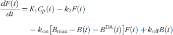
Based on the microdialysis literature cited above, we anticipated that intraperitoneal alcohol would induce a measurable increase in striatal DA. Figure 6 shows the fitting results for the striatum (left and right pooled together) of Rat A. The solid curves in Figure 6A and B constitute a representative “best fit” to the striatal PET data (solid circles) from the baseline and intraperitoneal alcohol conditions (fitted simultaneously according to Equation 8). Noise in the fitted curve for the alcohol condition (Figure 6B) is a direct consequence of noise in the cerebellum curve obtained in the same condition (cerebellar data are shown as open triangles). Figure 6D is the set of best DA curves according to the best-fit criteria described in Materials and Methods and thresholded at the detectability threshold of two times baseline. The mean peak time of the recovered DA curves is 18.27 ± 1.24 min post-[¹¹C]RAC injection (~29 min post alcohol challenge).

Figure 6.

Real rat data from alcohol experiment (Rat A). Pooled left and right striatum (filled circles) and cerebellum (triangles) data in the baseline (A) and activated states (B). Rat A received (0.5 g/kg ip) alcohol 11 min prior to scan. The smooth curves through the striatal points is one fit of the REF model to all the data in A and B simultaneously. The thin solid curves in A and B are the time derivatives of the cerebellum curves. Some noise in the fitted curves can be attributed to the noise in the cerebellum data which are used as the input. (C) Assumption of constant DA in rest condition. (D) The black curves are the resulting DA curves from best fits to the data in A and B. Note good temporal consistency of the best fits.

Figure 6D illustrates the consistency of the “best-fit” DA curves generated from this experiment. Notice particularly the great temporal coherence of the curves. The mean peak height for this experiment was found to be 3.79 ± 1.05 (=279% above basal DA). The latency of the DA response (i.e., DA takeoff time, t_D) in the animal's striatum was 8.79 ± 2.86 min following [¹¹C]RAC) (or ~20 min following intraperitoneal alcohol challenge). Mean values are based on 21 best fits culled from 77 converged.

Early Alcohol Experiment. The results of fitting the PET data from Rat B (left and right pooled) striatum are shown in Figure 7A (rest) and Figure 7B (activation). Analyzing these data yielded no DA curve (Figure 7D). Intraperitoneal alcohol was administered 2.5 hr before [¹¹C]RAC injection to look for prolonged effects of alcohol on either DA or possibly on receptor number. It has been speculated that internalization of D2/D3 receptors is part of the response to large doses of amphetamine [57] and that those internalized receptors are no longer available to bind to endogenous DA or to free raclopride. If that were the case with alcohol as well, then B_max would appear to be diminished, which might be detected by our model as increased DA. The ntPET results from Rat B suggest, preliminarily, that such is not the case.

We note that the fitted curves in Figure 7A and B (thick solid curves) look quite different in shape. These differences (i.e., the plateau in Figure 7B) can be traced to differences in the injections between the baseline and activation studies rather than to any alteration of kinetics by DA. The respective cerebellum curves (triangles) for each condition serve as indicators of the time course of tracer concentration in the plasma, which was more prolonged in the case of the activation condition for Rat B (Figure 7B). In summary, ntPET does not find any effect of alcohol administered 2.5 hr prior to the [¹¹C]RAC activation scan. This finding (Figure 7D) is consistent with microdialysis data that show dialysate DA levels returning to baseline within 120 min of administration of (2.0 g/kg) alcohol [19,22,25].

Figure 7.

Real rat data from delayed activation experiment (Rat B). Animal received intraperitoneal alcohol 2.5 hr prior to second scan. (A) Pooled data from the left and right striatum (filled circles) and the cerebellum (triangles) in the first rest (A) and in the “postactivation” state (B). The smooth curves through the striatal points is a fit of the REF model to all the data in A and B simultaneously. (C) Model assumption on DA at rest. (D) DA curves generated by best fits of model to data. Absence of any DA curve indicates that the model can fit data well without any need to invoke activation of DA, that is, there is no apparent long-term effect of intraperitoneal alcohol (1.5 g/kg) on the DA system.

Control Experiment

In this experiment, which combined two scans in the baseline condition, no increases in DA concentration were expected. Figure 8A and B shows the model-fitted PET curves to striatum TACs of the control animal (Rat C). The absence of a peak in Figure 8D indicates that the model required no DA activity at all to achieve a simultaneous fit of the data from both scans (relative peak height = 1 ± 0; based on 24 best fits out of 49 converged). Because the G parameter in the expression for free DA (Equation 5) was constrained to be non-negative, we were only looking for positive excursions of the DA curve that would explain the data. This is, however, the correct way to analyze the control because the real alcohol challenge and simulation data were also fitted by limiting G to non-negative values (i.e., we only looked for transient rises in DA during the activation scan in response to a stimulus).

Discussion

We have demonstrated that ntPET—a new method for identifying and characterizing temporal characteristics of neurotransmitter release induced by a stimulus—is a feasible analysis for use with dynamic small-animal imaging. We have named our new method ntPET (neurotansmitter PET) to emphasize the analogy with fMRI (functional MRI), a method for finding temporal patterns in dynamic MR data. We have no doubt that human imaging will yield even better (more precise) results and even lower detectability thresholds due to better signal-to-noise ratios in the TACs. Although we chose to focus on the dopaminergic system, this method can be applied to other neurotransmitter systems as well, given a displaceable radioligand that competes observably with the particular neurotransmitter of interest. Just as we expect human data to be even more amenable to ntPET analysis, we anticipate that further advances in sensitivity and spatial resolution for small-animal scanners will lead to more precise DA parameter estimates and lower incidences of false positives of any kind. Tests with multiple simulations of rat data (allowing for variation across subjects) show that the temporal precision of ntPET (i.e., the ability to locate and resolve DA peaks in time) may be as good as 2–4 min. We cannot say anything about the true shape of the DA curve in experimental data because we have fixed our choice of DA curves to be those of the family of gamma-variate curves consistent with Equation 5.

Based on simulations, the uncertainty in estimates of DA parameters for any given dataset appears to be in the range of 1 min. The precision of the estimates for Rat A is consistent with this assessment. Recall that across simulations, the tracer parameters used to create the data were varied by ±10%. Within datasets, only the noise accounts for variability in the estimates. Hence, we would expect greater variability across subjects than within subjects.

Figure 8.

Real rat data from a control experiment (Rat C). (A) Pooled data from the left and right striatum (filled circles) and the cerebellum (triangles) in the first rest (A) and in the second rest state (B). The smooth curves through the striatal points is a single fit of the REF model to all the data in A and B simultaneously. (C) Model assumption on DA at rest. (D) DA curves generated by best fits of model to data. Absence of any DA curve indicates the model can fit data well without any need to invoke activation of DA.

The null case analyses allow us to set detectability thresholds for our method. The simulations and fits of 98 null cases (there was no DA release included in the simulated data) suggest that artifactually recovered DA responses due to noise in the data will be acceptably rare over a defined time window from 5 to 50 min (~10%) or 5 to 45 min (~5%) of the scan. For noise levels comparable to our rat data presented here, we can safely say that any peak DA response that exceeds our threshold (100% above baseline) in the window between 5 and 45 min of the scan is unlikely to be merely the model's attempt to fit noise spikes in the activation scan data and therefore is likely to correspond to an actual release of synaptic DA. One need not be troubled by “throwing away” subthreshold responses that are generated by the present method. By way of comparison, we cite the example of multilead EEG, another mathematical inverse method, used to generate hundreds of dipoles (“source localization”) in the brain from potentials recorded on the skull, only to have most of them thresholded away as being unphysiological or likely due to noise. We fully admit that experimental variables other than alcohol could cause DA to be elevated. To rule out all of these factors (e.g., stress of injection), we will need to replicate and expand on our array of control experiments.

Our predictions of false positives based on null case simulations may, in fact, be overly cautious. (1) We note that only 1 time out of 98 was the peak of a false result recovered within a few minutes of the time that we observed the peak DA response to alcohol in Rat A. (2) Bonafide DA responses tend to be much more robust (higher) and temporally coherent (greater agreement among “best” fits) when there is really a DA curve to be found than when there is none. Thus, we predict that it will be unlikely that a false response due to noise alone will be confused with real DA activation. In the future, we may be able to improve our ability to reject false fits by incorporating a penalty on incoherence (high standard deviation) of the peak time and peak height estimates.

Comparison with Microdialysis Data

Our preliminary finding that ntPET recovered an alcohol-induced striatal DA response that peaked 29 min post alcohol administration is perfectly consistent with the findings in several microdialysis and voltammetry studies in both anesthetized [24,26] and freely moving animals [18,20,22,25,27]. We are optimistic that the method will prove to be a valuable tool for probing the second-to-minute time scale for temporal aspects of dopaminergic responses to pharmacological challenges in preclinical experiments. The believability of our findings in Rat A are bolstered by the lack of finding in Rat B (alcohol long before the scan) or in Rat C (no alcohol in either scan).

To put the results from our alcohol challenge experiments into context, we present our findings for Rat A superimposed on published microdialysis results derived from an experimental setup very similar to ours (see Figure 9). Heidbreder and De Witte [26] assayed for DA in microdialysis samples from the nucleus accumbens of rats following 1.0 g/kg ip alcohol. Like our rats, theirs were anesthetized. Consistent with our Rat A data, the average DA response as measured by microdialysis peaked in the 20–40 min time bin (post alcohol). Of course, microdialysis sampling is very slow which is reflected in the width (20 min each) of the bars in Figure 9. This figure is our reformatting of the data in Figure 1 of Heidbreder. Because their data were based on 21 rats, it is quite reasonable to expect that the bars reflect interanimal variability in take off and peak time. One can easily imagine that the bar graph in Figure 9 is the average of many results such as Rat A, some of whom would have takeoff and peak times earlier and broader, and others would have been later and sharper than Rat A. It is also not unreasonable that the ntPET result for Rat A peaks at a higher fraction of baseline than does the “peak” (20–40 min) microdialysis measurement in Figure 9 aside from interanimal variation. Although it is true that the placement of microdialysis probes can be targeted to a particular nucleus (e.g., precisely in the nucleus accumbens), whereas the PET signal is based on an ROI encompassing the whole striatum (which would tend to dilute any local effect that originates in a small striatal subregion), there are many obstacles to microdialysis sampling that might cause it to detect lower effective concentrations of DA than ntPET. As stated above, the PET signal responds to competition at the D2/D3 receptors which are largely, if not exclusively, intrasynaptic. The microdialysis probe is distant from the synapse and so it will only detect DA that manages to (a) diffuse out of the synapse (b) avoid uptake by DA transporters, (c) avoid metabolism by catechol-O-methyltransferase and other enzymes, and (d) diffuse across the probe membrane. Not only will there be a considerable gradient between the high intrasynaptic concentration and the lower extracellular one, but the insertion of the microdialysis probe causes disruption of the tissue that creates a further concentration gradient from the unaffected tissue down to a yet lower concentration at the probe membrane surface [58].

Figure 9.

DA response to alcohol in striatum of Rat A measured by ntPET compared with published microdialysis results. Abscissa is time (min) from dose of alcohol. Gray bars are adapted from Figure 3 of Heidebreder and deWitte (1993) who used assayed extracellular DA in the nucleus accumbens via microdialysis in 21 anesthetized rats following 1.0 g/kg alcohol ip. Width of bars is 20 min because microdialysis sampling technique used required 20 min per sample. Note nearly perfect agreement between our Rat A and the group of rats studied by Heidebreder. Note also that with ntPET we can localize the DA peak time of an individual rat to within 25 sec, whereas this type of microdialysis assay can only locate the average peak of the group to within 20 min.

Given the temporal variability between rats' DA responses that we postulate with regard to the Heidbreder data, it is also possible that reanalyzing previously published studies in humans and animals with the present method would reveal considerable temporal variation in neurotransmitter dynamics across subjects. If the hypothesized variability in temporal responses of the DA system to drugs is borne out (after scanning many subjects), and our method continues to perform with better than 4 min uncertainty in the estimate of DA timing, then we believe this represents an opportunity to delve deeper than previously possible into the neurochemical workings of the brain.

Spatial Resolution Limitations

A consequence related to the limited spatial resolution of PET may be that our images will necessarily suffer from partial volume (PV) error, and therefore, our TACs may not reflect the true shape of the concentration of tracer in a given tissue over time. We have not yet investigated the effect of PV error on recovery of DA curves. It seems likely that such an error, if uncorrected, could lead to a bias in DA timing parameter estimates but not to outright false positives. For one thing, whatever effect of PV exists, it is present during both scans. Thus, even if uncorrected data yield biased timing results, it is our expectation that the bias will be fairly consistent across time and across scans and that early neurotransmitter release will be distinguishable from late release. We must emphasize that standard analysis methods that rely on differences in BP are unable even to make such early versus late distinctions. As we continue to refine our method, it will be important to assess the impact of PV error and to explore the use of established correction methods in conjunction with the ntPET methodology presented here.

Model Assumptions

Our model is built on certain assumptions such as the constancy of tracer parameters, Θ_RAC, across conditions. This would seem not to be too restrictive as long as the animal is scanned twice within a reasonable period (perhaps 1–2 weeks) in a well-controlled environment and at the same time of day. Strictly speaking, a violation of this assumption would be caused by an alteration to blood flow due to drug, but even this violation would not necessarily lead to artifacts. Comparable change in K₁ and k₂ would not affect the shape of the TACs appreciably [3,4], whereas a decoupled change in one without a change in the other is probably unphysiological. An implicit assumption of the model is that the neurotransmitter and the tracer obey competitive binding rules at the receptor site. Anything that would cause this condition to be violated might invalidate the model. If significant numbers of receptors were internalized or otherwise became inaccessible to DA while remaining bound to raclopride (or vice versa), the method might fail. From a modeling standpoint, one might address such a phenomenon—if it were reliably demonstrated—by incorporating a concentration- or time-dependency into the model term for available receptors. Frankly, though, we are probably at the limit of allowable number of parameters already. Outside the need for constancy of tracer parameters across conditions, we note that all PET methods and models are potentially invalidated by time-varying parameters or noncompetitive binding when these phenomena are assumed not to occur.

Parameter Identifiability

Our model, a reference region (REF) formulation of the enhanced endogenous tracer kinetic model (Figure 1), contains a large number (10) of unknown parameters compared to typical PET kinetic models. With so many parameters being estimated, it is proper to question if they can each be uniquely identified. One must bear in mind, the primary goal of ntPET is to identify uniquely the temporal parameters of the DA function (Equation 5). Our results with simulations and real data are the appropriate tests for feasibility and from a theoretical standpoint, we are confident in our estimates for four reasons: (i) We are primarily interested in parameters that govern DA timing. For us, Θ_RAC and Θ_REF are “nuisance” parameters. (ii) We observe the system in two conditions: baseline and stimulus, but fit all the data simultaneously. (iii) We add a prior (i.e., a penalty function) to the objective function to limit the search space for feasible parameter choices. (iv) It can be demonstrated that the sensitivity of the PET signal (baseline and activation data together) to changes in DA parameters is distinct from its sensitivity to changes in tracer parameters [59]. There are other ways of improving parameter identifiability and precision that we are currently investigating. One way is to impose tighter bounds or other penalties on the estimates of some parameters based on literature values. Another may be to acquire arterial blood samples to get a better estimate of the plasma input function [60].

Conclusions

We demonstrate the feasibility of noninvasive recovery of DA kinetics in the rat striatum following an intraperitoneal alcohol (or other drug) challenge. This information is not available from standard PET imaging studies which use changes in apparent BP before and after challenge to infer average concentrations of DA. Results from our numerous simulation case studies suggest that the kinetic parameters describing DA release can be estimated accurately and precisely, and that the observed DA responses are unlikely to have happened by chance. The new parameter estimation method we introduce for probing neurotransmitter fluctuations (“ntPET”) requires dynamic PET data in two conditions, is noninvasive, reflects intrasynaptic neurotransmitter activation, and has at least 1- to 2 min (within-subject) temporal resolution. Our efforts to validate this new method in small animals will continue with experiments using different drugs and routes of administration known to result in temporally distinct increases in DA concentration. ntPET should achieve even more precise estimates of neurotransmitter timing when applied to higher quality human data (better signal-to-noise ratio). The new method that we present possesses clear advantages over the invasive probe-based approaches presently used in preclinical neurochemical research. Given the potential precision of ntPET, we foresee the ability to identify and discriminate different temporal patterns in neurotransmitter release induced by pharmacological and possibly behavioral stimuli.