Sage Journals: Discover world-class research

Abstract

The cancer mortality ratios (CMRs) in Poland in high and low level radiation areas were analyzed based on information from national cancer registry. Presented ecological study concerned six regions, extending from the largest administration areas (a group of voivodeships), to the smallest regions (single counties). The data show that the relative risk of cancer deaths is lower in the higher radiation level areas. The decrease by 1.17%/mSv/year (p = 0.02) of all cancer deaths and by 0.82%/mSv/year (p = 0.2) of lung cancers only are observed.

Keywords

ecological study epidemiology low dose hormesis Poland residential

INTRODUCTION

High-background radiation areas (HBRA) can be found in many places worldwide (Wei et al. 1997; Jaworowski 2001; Hendry et al. 2009). Such places can also be found in Poland. A common question, to the best of the authors’ knowledge not considered for Poland, is whether there is a relationship between the natural level of ionizing radiation and corresponding rates of cancer mortality.

The average annual effective dose in Poland equals 2.48 mSv from natural sources (GUS 2007). 54.9% of the background dose is derived from the radioactive gas radon, 18.6% from gamma rays and 26.5% from other origins (e.g. cosmic rays and in-body radionuclides) (GUS 2007). The main geographical differences between annual doses in various places are due to radon and gamma sources. The extra contribution from man-made sources (mostly medical) is not taken into account in these considerations.

The major administrative division of Poland (since 1999) contains 16 voivodeships (provinces). Each voivodeship¹ is divided into several counties (powiats). Some of them are city-counties. Each of them has their own medical statistical registry of local population. Based on this available information, one can study the potential correlation between local annual effective dose from natural sources and cancer mortality ratio (CMR).

SOURCES AND METHODS

The data containing annual effective doses in various regions of Poland come from the Radiation Atlas of Poland (RAP 2005), which contains information about average doses, separately from indoor radon and gamma rays in each voivodeships. The same data, but in single counties, can be inferred from the maps in Geochemical Atlas of Poland (AGP 1995) and in Radioecological Maps of Poland (MRP 1995).

Data concerning deaths from all causes and from cancer deaths were obtained from the Central Statistical Office (GUS 2007, 2011). The registry based on the modern voivodeships system contains data from 1999 to 2009, and data at the level of individual counties are available for the period of 1999 to 2007.

Six sets of data were analyzed:

Set 1 – taking two groups of 5 voivodeships: the ones with the highest (more than 2.5 mSv/year) average annual effective dose (Dolnoślaͅskie, Małopolskie, Opolskie, Podkarpackie and Ślaͅskie voivodeships) and the ones with the lowest (less than 2.4 mSv/year) dose (Lubuskie, Lódzkie, Pomorskie, Wielkopolskie and Zachodniopomorskie voivodeships); the statistical data are presented in Table 1; see also Fig. 1;

TABLE 1.

The original statistical data for each set from 1 to 6 (GUS 2011; RAP 2005; AGP 1995; MRP 1995); LB – low background area; HB – high background area.

	Set 1		Set 2		Set 3		Set 4		Set 5		Set 6

	Dolnoślaͅskie, Małopolskie, Opolskie, Podkarpackie, Ślaͅskie voivodeships (HB)	Lubuskie, Łódzkie, Pomorskie, Wielkopolskie, Zachodniopomor skie voivodeships (LB)	Dolnoślaskie and Małopolskie voivodeships (HB)	Lubuskie and Zachodniopomor skie voivodeships (LB)	Małopolskie voivodeship (HB)	Zachodniopomor skie voivodeship (LB)	First group of counties: Jelenia Góra, Jeleniogórski, Kamiennogórski, Nowotarski, Tatrzański (HB)	Second group of counties: Goleniowski, Krośnieński, Policki, Świnoujście, Żagański (LB)	Jelenia Góra and Jeleniogórski counties (HB)	Świnoujście and Policki counties (LB)	Jelenia Góra city-county (HB)	Świnoujście city-county (LB)
Total population (in 2009 only)	13 948 451	10 883 457	6 174 897	2 703 245	3 298 270	1 693 198	444 450	327 578	148 429	109 852	84 564	40 765

Total number of deaths from all causes between 1999 and 2009/2007 ^‡	1 447 814	1 161 096	635 112	268 434	317 980	167 992	36 439	25 029	14 507	6 757	8 444	3 192

Total number of cancer deaths between 1999 and 2009/2007 ^‡	359 764	292 811	160 165	69 906	79 927	44 502	8 628	6 274	3 551	1 832	2 128	925

Average concentration of indoor radon [Bq/m³] ^∗	54 ± 24 ^∗∗	30 ± 13	61 ± 30	22 ± 11	70 ± 24	21 ± 13	117 ± 51 ^†	18 ± 8 ^†	121 ± 63 ^†	16 ± 8 ^†	121 ± 63 ^†	9 ± 5 ^†

Average dose rate of gamma radiation [nGy/h] ^∗	83 ± 33	69 ± 25	86 ± 35	69 ± 28	85 ± 25	70 ± 35	57 ± 19 ^†	19 ± 12 ^†	77 ± 21 ^†	18 ± 12 ^†	85 ± 20 ^†	16 ± 12 ^†

Additional comment	–	–	–	–	main city: Kraków (Cracow)	main city: Szczecin (Stettin)	–	–	–	–	elevation above mean sea level: 347 m	at elevation above mean sea level: 5 m

∗

all uncertainties show one standard deviation (68% CI) (see text for details)

∗∗

there are no data of radon concentration in Podkarpackie voivodeship

†

estimated values from (AGP 1995; MRP 1995; RAP 2005)

‡

2009 for voivodeships (sets 1–3) and 2007 for counties (sets 4–6)

FIGURE 1.

The map of selected Polish voivodeships: the higher radiation ones (D means Dolnoślaͅskie, O-Opolskie, S-Ślaͅskie, M-Małopolskie, Pk-Podkarpackie) and lower radiation ones (Ld-Łódzkie, W-Wielkopolskie, L-Lubuskie, Z-Zachodniopomorskie, Pm-Pomorskie)

Set 2 – comparing two pairs of voivodeships: the one with the highest (more than 2.9 mSv/year) average annual effective dose (Dolnoślaͅskie and Małopolskie voivodeships) and the one with the lowest (less than 1.95 mSv/year) dose (Lubuskie and Zachodniopomorskie voivodeships) - the data are presented in Table 1;

Set 3 – taking two single voivodeships: the one with the maximal value of average annual effective dose (3.35 mSv/year, the Małopolskie voivodeship) and the one with the minimal value of average annual effective dose (1.85 mSv/year, the Zachodniopomorskie voivodeship) - the statistical data are presented in Table 1;

Set 4 – comparing two groups of 5 counties: the first group (Jelenia Góra, Jeleniogórski, Kamiennogórski, Nowotarski and Tatrzański counties) with the average annual effective dose higher than 4 mSv/year, and the second group (Goleniowski, Krośnieński², Policki, Świnoujście and Żagański counties) with the dose lower than 1.4 mSv/year - the statistical data are presented in Table 1; see also Fig. 2;

FIGURE 2.

The map of selected Polish counties; black – high radiation; grey – low radiation

Set 5 – comparing two pairs of counties: Jelenia Góra (city-county) and Jeleniogórski counties with the average annual effective dose higher than 4.6 mSv/year, and the Świnoujście (city-county) and Policki counties with the dose lower than 1.3 mSv/year; the statistical data are presented in Table 1;

Set 6 – comparing two city-counties: Jelenia Góra with the maximal average annual effective dose of 4.75 mSv/year, and the Świnoujście with the minimal dose of 1.06 mSv/year - the statistical data are presented in Table 1.

The values of average annual effective dose (from the natural origin only) in each region were calculated as a result of summarizing:

the dose derived from the local average concentration of indoor radon as the largest fraction of the whole dose;

the dose derived from the gamma radiation (usually from the ground);

the constant dose of 0.66 mSv/year derived from the contributions of cosmic rays (42.9%), in-body radionuclides (41.8%), and thoron (15.3%).

Doses from radon concentration are calculated using the Central Statistical Office's (GUS 2007) conversion factor: 1 Bq/m³ = 0.028 mSv/year effective dose to the whole body. However, one can find also a little lower factor (1 Bq/m³ = 0.022 mSv/year) estimated from a equivalent dose to lungs from radon (Fornalski and Dobrzyński 2011; UNSCEAR 2006). The choice of multiplication factor has no influence on final conclusions. The doses from radon concentration and gamma radiation for each of the voivodeships are calculated from RAP (2005). The level of gamma radiation for each county (data sets 4–6) was estimated from (AGP 1995; MRP 1995) ³. The radon concentrations in data sets 4–6 were estimated from the Ra-226 concentration (AGP 1995; MRP 1995). Information about uncertainties of radon concentrations and dose-rates come from private correspondence with Central Laboratory for Radiological Protection and Chief Inspectorate of Environmental Protection, and are presented in Table 1. The total uncertainties of radiation exposures (horizontal error bars in Figs 4 and 5) were calculated using standard methods of error propagation.

All results are presented as CMR for cancer deaths, defined as the result of dividing the number of cancer deaths by the number of deaths from all causes⁴. The mortality (number of deaths) is a simple average, not age or gender adjusted. The aftermath of CMR values are relative risks (RR) and absolute increases of cancer mortality (explained in the description of Table 2). All values are shown with uncertainties of one standard deviation (68% CI, confidence intervals⁵). The same convention of one standard deviation is used for all values of doses’ uncertainties.

TABLE 2.

Raw results without adjustment on confounding factors.

	Lower level of radiation			Higher level of radiation				Absolute increase of cancer deaths^†† [%]		Relative risk (RR)^§ [%]
	Effective dose^† [mSv/year]	CMR [%] all cancers	CMR [%] lung cancers	Effective dose^† [mSv/year]	CMR [%] all cancers	CMR [%] lung cancers	Excess effective dose^†† [mSv/year]	all cancers	lung cancers	all cancers	lung cancers
Set 1^∗	2.12 ± 0.59	25.2 ± 0.1	23.6 ± 0.1	2.88 ± 0.97	24.8 ± 0.1	22.9 ± 0.1	0.76 ± 0.38	−0.4 ± 0.2^c	−0.7 ± 0.2^c	98.5 ± 0.3^c	97.0 ± 0.6^c
Set 2^∗	1.89 ± 0.57	26.0 ± 0.2	25.3 ± 0.3	3.10 ± 1.15	25.2 ± 0.1	23.6 ± 0.2	1.21 ± 0.59	−0.8 ± 0.3^c	−1.7 ± 0.4^c	96.8 ± 0.5^c	93.3 ± 1.0^c
Set 3^∗	1.85 ± 0.68	26.5 ± 0.2	25.7 ± 0.3	3.35 ± 0.90	25.1 ± 0.2	22.4 ± 0.2	1.5 ± 0.22	−1.4 ± 0.3^c	−3.3 ± 0.4^c	94.9 ± 0.7^c	87.2 ± 1.2^c
Set 4^∗	1.32 ± 0.34	25.1 ± 0.4	26.9 ± 0.8	4.42 ± 1.60	23.7 ± 0.3	22.9 ± 0.6	3.1 ± 1.26	−1.4 ± 0.5^c	−4.0 ± 1.0^c	94.5 ± 1.8^c	85.1 ± 3.2^c
Set 5^∗	1.26 ± 0.34	27.1 ± 0.8	27.5 ± 1.4	4.68 ± 1.95	24.5 ± 0.5	25.4 ± 1.0	3.42 ± 1.61	−2.6 ± 1.0^c	−2.1 ± 1.8^b	90.3 ± 3.0^c	92.4 ± 5.8^b
Set 6^∗	1.06 ± 0.26	29.0 ± 1.1	28.8 ± 2.1	4.75 ± 1.94	25.2 ± 0.7	24.5 ± 1.2	3.69 ± 1.69	−3.8 ± 1.4^c	−4.3 ± 2.5^b	87.0 ± 3.9^c	85.1 ± 7.3^c

∗

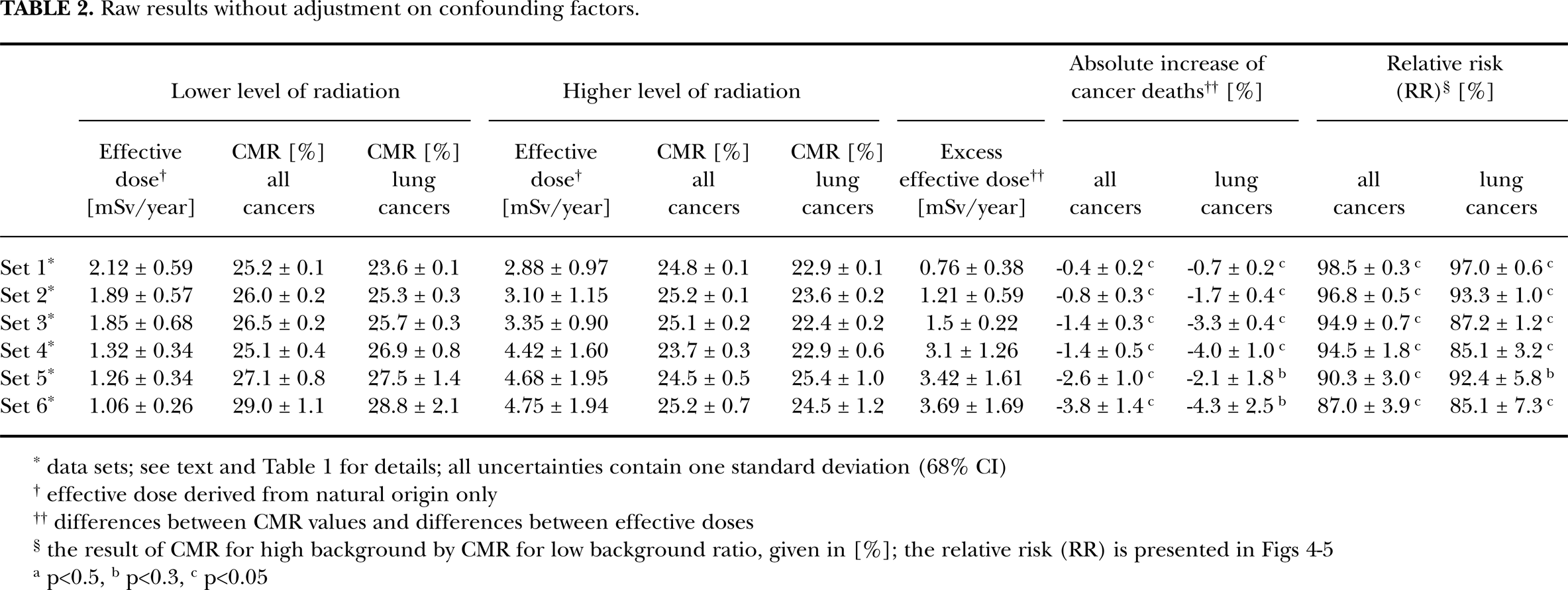
data sets; see text and Table 1 for details; all uncertainties contain one standard deviation (68% CI)

†

effective dose derived from natural origin only

††

differences between CMR values and differences between effective doses

the result of CMR for high background by CMR for low background ratio, given in [%]; the relative risk (RR) is presented in Figs 4–5

p<0.5,

p<0.3,

p<0.05

UNADJUSTED RESULTS

All raw (unadjusted) results are summarized in Table 2, for each data set from 1 to 6, and are discussed below. The average annual doses of natural radiation were calculated always from the known radon concentration and gamma radiation that are displayed in Table 1. The average human lifetime was assumed to be 75 years.

Set 1 – two groups of voivodeships

The average annual effective dose, inferred from Table 1, amounts to (2.88 ± 0.97) mSv/year in the first group of voivodeships (higher background, HB). This is compared with (2.12 ± 0.59) mSv/year in the second group (lower background, LB). During the human lifetime the difference in cumulative doses between these groups is 58 mSv.

The cancer mortality ratio in the higher background group of voivodeships, calculated as an average from the year 1999 to 2009 (Table 1), is CMR = (24.8 ± 0.1) % compared to the second group of voivodeships where CMR = (25.2 ± 0.1) %. The difference in CMRs in both groups (0.4 ± 0.2) % is statistically significant.

Set 2 – two pairs of voivodeships

The average annual effective dose inferred from Table 1 amounts to (3.10 ± 1.15) mSv/year in the two higher background voivodeships (Dolnoślaͅskie and Małopolskie) and (1.89 ± 0.57) mSv/year in the lower background group. During the human lifetime the difference in cumulative doses between these groups is 91 mSv.

The cancer mortality ratio in the higher background pair of voivodeships, calculated as an average from the year 1999 to 2009 (Table 1), is CMR = (25.2 ± 0.1) % compared to the second pair of voivodeships where CMR = (26.0 ± 0.2) %. The difference in CMRs (0.8 ± 0.3) % is statistically significant.

Set 3 – two voivodeships

The average annual effective dose inferred from Table 1 for Malopolskie voivodeship is (3.35 ± 0.90) mSv/year. Analogically, annual effective dose in Zachodniopomorskie voivodeship is (1.85 ± 0.68) mSv/year. During the human lifetime the difference in cumulative doses between these voivodeships is 112 mSv.

The cancer mortality ratio in Malopolskie voivodeship (higher background), calculated as an average from the year 1999 to 2009 (Table 1), is CMR = (25.1 ± 0.2) % compared to the Zachodniopomorskie voivodeship (LB) where CMR = (26.5 ± 0.2) %. The difference between CMRs (1.4 ± 0.3) % is statistically significant. The temporal evolution of these results is presented in Fig. 3, for the time period from 1999 to 2009.

FIGURE 3.

The time evolution of the cancer mortality ratios (CMR) for two Polish voivodeships (data set 3): Małopolskie (dark pillars; effective dose 3.35 mSv/year) and Zachodniopomorskie (bright pillars; effective dose 1.85 mSv/year) from the year 1999 to 2009

Set 4 – two groups of counties

The average annual effective dose inferred from Table 1 for the high background group of counties (Jelenia Góra, Jeleniogórski, Kamiennogórski, Nowotarski and Tatrzański county) is (4.42 ± 1.60) mSv/year compared to the second group (LB) of counties (Goleniowski, Krośnieński, Policki, Świnoujście and Żagański county) having an effective dose of (1.32 ± 0.34) mSv/year. During the human lifetime the difference in cumulative doses between these groups of counties is 233 mSv.

The cancer mortality ratio in the high background group of counties, calculated as an average from the year 1999 to 2007 (Table 1), is CMR = (23.7 ± 0.3) % compared to the second group of counties where CMR = (25.1 ± 0.4) %. The difference between CMRs (1.4 ± 0.5) % is statistically significant.

Set 5 – two pairs of counties

The average annual effective dose inferred from Table 1 for the high background pair of counties (Jelenia Góra and Jeleniogórski) is equal (4.68 ± 1.95) mSv/year compared to the second pair of LB counties (Świnoujście and Policki) having an effective dose of (1.26 ± 0.34) mSv/year. During the human lifetime the difference in cumulative doses between these pairs of counties is 257 mSv.

The cancer mortality ratio in the high background pair of counties, calculated as an average from the year 1999 to 2007 (Table 1), is CMR = (24.5 ± 0.5) % compared to the second pair of counties where CMR = (27.1 ± 0.8) %. The difference between CMRs in both (2.6 ± 1.0) % is statistically significant.

Set 6 – two counties

The average annual effective dose inferred from Table 1 for Jelenia Góra (high background) city-county is equal (4.75 ± 1.94) mSv/year compared to the Świnoujście city-county having an effective dose of (1.06 ± 0.26) mSv/year. During the human lifetime the difference in cumulative doses between these counties is 277 mSv.

The cancer mortality ratio in the Jelenia Góra city-county, calculated as an average from the year 1999 to 2007 (Table 1), is CMR = (25.2 ± 0.7) % compared to the Świnoujście city-county where CMR = (29.0 ± 1.1) %. The difference between CMRs in both (3.8 ± 1.4) % is statistically significant.

Summary of the unadjusted results

All the unadjusted results for all cancers and lung cancers only are summarized in Table 2 and Figs 4 and 5. The straight line regression fit to the RR data (Figs 4–5 and Table 2) results in a decrease of all cancer mortality by 3.07%/mSv/year (p = 0.0003; χ² = 1.8) ⁶, and by 7.37%/mSv/year (p = 0.0001; χ² = 5.0) for lung cancers only. All fitting parameters are presented in Table 5.

FIGURE 4.

The final results for mortality due to all cancers . The vertical axis presents the relative risk (RR) while the horizontal axis presents the differences in effective doses in all six data sets. The round dots mean the unadjusted results (from Table 2) while the square points mean the adjusted results (from Table 4). The dashed line abbreviated by LNT shows expectations based on the linear no-threshold assumption in risk prediction (Sanders 2010). Dash-dot lines are best fits (Table 5) to the both types of data. The uncertainties (both for RR and doses) show one standard deviation (68% CI). See Sources and Methods section as well as Tables 2 and 4 for details concerning uncertainties. ^∗the empty squares results are potentially biased because of assumed information about smokers (see text for details)

FIGURE 5.

The final results for lung cancers ’ mortality. The vertical axis presents the relative risk (RR) while the horizontal axis presents the differences in effective doses in all six data sets. The round dots show the unadjusted results (from Table 2) while the square points the adjusted ones (from Table 4). The dashed line abbreviated by LNT shows expectations based on the linear no-threshold assumption in risk prediction (Sanders 2010). Dash-dot lines are best fits (Table 5) to the both types of data. The uncertainties (both for RR and doses) show one standard deviation (68% CI). See Sources and Methods section as well as Tables 2 and 4 for details concerning uncertainties, ^∗the empty squares results are potentially biased because of assumed information about smokers (see text for details)

TABLE 3.

The data on potential confounding factors; LB - low background area; HB - high background area.

	Set 1		Set 2		Set 3		Set 4		Set 5		Set 6

	LB	HB	LB	HB	LB	HB	LB	HB	LB	HB	LB	HB
People age 70 or older [%] ^a,∗	9.3	9.9	8.9	10.0	9.0	10.0	7.7	9.6	6.5	11.0	8.6	11.8
Longevity (men/women) [years] ^a,∗	71.2/79.6	71.9/80.0	70.9/79.5	72.1/80.3	71.0/79.5	73.1/81.1	no data	no data	no data	no data	no data	no data
Regular daily smokers (men/women) [%] ^b
in 2004	36/22	33/19	37/24	32/18	37/25	31/14	no data	no data	no data	no data	no data	no data
in 1996	43/23	40/17	45/26	41/20	47/28	38/16	no data	no data	no data	no data	no data	no data
Percent of lung cancer deaths among all cancer deaths [%] ^c	23.6	22.9	25.3	23.6	25.7	22.4	26.9	22.9	27.5	25.4	28.8	24.5
Migration [%] ^a,∗
into	0.79	0.70	0.82	0.74	0.82	0.68	1.48	0.78	2.53	1.30	1.25	1.13
out	0.78	0.71	0.87	0.66	0.88	0.57	1.04	0.79	1.24	1.29	1.16	1.39
Unemployment [%] ^a,∗	13.5	13.8	22.2	12.0	28.3	8.6	16.6	11.6	11.3	14.0	11.4	11.6
Higher educated (in 2002 only) [%] ^a	9.7	9.5	9.5	10.2	10.2	10.2	7.7	7.6	11.1	10.5	11.6	12.9
Personal income per month netto [EUR] ^a,∗	259	246	260	255	263	241	no data	no data	no data	no data	no data	no data
Annual regional budget (expenditure) per capita [EUR] ^a,∗	137	110	160	116	149	105	268	285	501	561	1027	845
Annual environmental pollution per capita (emission from industry) ^a,∗
air (gas) [kg/year]	28	68	22	36	20	42	28	3	69	6	10	7
air (dust) [kg/year]	1.6	1.9	1.9	1.5	2.2	1.3	5.1	0.5	10.8	0.8	9.0	0.3
water [g/year]	174	346	209	306	291	133	1429	14^†	4161	32^†	49	no data

data from (GUS 2011)

data from (Wojtyniak and Gorynski 2008)

data from (KRN 2011)

∗

in the last year of the analysis

†

the value can be understated because there are no data from Jelenia Góra

TABLE 4.

Adjustment factors and results after adjustement.

Adjustment to CMR [%] ^∗								Absolute increase of cancer deaths [%] ^∗∗		Relative risk (RR) [%] ^∗∗

	Longevity	Smoking: all cancers	Smoking: lung cancers	Education	Air pollution	Unemployment	Economic status	all cancers	lung cancers	all cancers	lung cancers
Set 1	−0.42	0.9	1.5	−0.02	−0.01	0	−0.37	−0.3 ± 0.2^b	0.0 ± 0.3^a	98.8 ± 0.5^a	99.9 ± 1.0^a
Set 2	−0.77	1.65	2.75	0.08	−0.01	0.1	−0.57	−0.3 ± 0.3^a	−0.1 ± 0.5^a	98.7 ± 0.9^b	99.6 ± 1.7^a
Set 3	−0.7	2.55	4.25	0	−0.01	0.2	−0.63	+0.1 ± 0.3^a	−0.2 ± 0.6^a	100.2 ± 1.1^a	99.3 ± 2.1^a
Set 4	−1.33	1.65^†	2.75^†	−0.01	0.17	0.05	0.09	−0.8 ± 0.8^b	−2.3 ± 1.6^b	96.9 ± 3.1^b	91.5 ± 5.6^b
Set 5	−3.15	2.55^†	4.25^†	−0.07	0.22	−0.03	0.16	−2.9 ± 1.4^a	−0.7 ± 2.8^a	89.1 ± 4.9^a	97.4 ± 10.0^a
Set 6	−2.24	2.55^†	4.25^†	0.16	0.09	0	−0.32	−3.5 ± 2.1^b	−2.4 ± 3.9^a	87.8 ± 6.5^b	91.8 ± 12.6^a

∗

the presented values were added to the HB's CMRs (Tab. 2); see Tab. 3 and text for details

∗∗

see Tab. 2 for details; results for sets 4–6 can be potentially biased^†

†

results can be potentially biased; information about smokers for sets 4–6 was approximated from general voivodeships statistics (set 2 and 3), because there are no data for single counties (Tab. 3)

p<0.5,

p<0.3,

p<0.05

TABLE 5.

The fitted^† slopes [%/mSv/year] for the adjusted (Table 4) and unadjusted (Table 2) data; uncertainties represent one standard deviation (68% CI, confidence intervals).

	Absolute increase of cancer deaths [%/mSv/year] (68% CI)		Relative risk^‡ (RR) [%/mSv/year] (68% CI)

	adjusted results^∗	unadjusted results^∗∗	adjusted results^∗	unadjusted results^∗∗
all cancers	−0.30 (−0.45; −0.09) (χ² = 2.8; p=0.08)	−0.77 (−0.90; −0.44) (χ² = 1.5; p=0.01)	−1.17 (−1.51; −0.60) (χ² = 6.3; p=0.02)	−3.07 (−3.43; −2.18) (χ² = 1.8; p=0.0003)
lung cancers	−0.19 (−0.48; +0.14) (χ² = 0.8; p=0.3)	−1.80 (−2.04; −1.18) (χ² = 3.7; p=0.002)	−0.82 (−1.55; +0.10) (χ² = 1.7; p=0.2)	−7.37 (−8.14; −5.40) (χ² = 5.0; p=0.0001)

†

classical method of least squares parameter estimation with two degrees of freedom (effective dose uncertainties taken into consideration)

‡

results presented in Figs 4 and 5

∗

see Table 4

∗∗

see Table 2

ADJUSTED RESULTS

All results presented in Table 2 can be potentially biased (Bogen 1999; Bogen 2001; Bogen and Cullen 2002) because of many confounding factors (like average age, smoking, economic differences etc.) that could deform presented conclusions. Poland, as many European countries, is a rather homogeneous state, with weak regional differences in social and economic status, medical standards, race, religion etc. Nevertheless, in attempt to understand how such factors may be important, Table 3 presents statistical data about many potential confounding factors found in presented six sets of regions.

All confounding factors from Table 3 can be subdivided into following groups:

Inhabitants’ age

Table 3 contains two information about inhabitants’ age: the longevity (in years) of local population (available only for voivodeships; sets 1–3), and the percent of inhabitants in the age of 70 or older (available for all sets 1–6). It seems necessary to find the relationship between both types of data mentioned above, especially between differences in high (HB) and low (LB) background areas. Let us define the average longevity (in years) as:

L = F_{M} L_{M} + (1 - F_{M}) L_{W}

(1)

where F_M means the fraction of men, while L_M and L_W denote the longevity of men and women, respectively, taken from the second line of Table 3. In addition, if the data in the first line (for people in the age of 70 or older) are denoted as A₇₀ , the differences between HB and LB areas can be used to calculate the factor C:

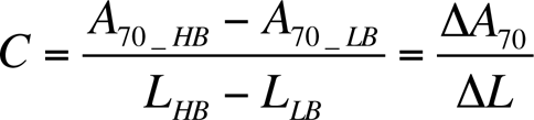
C = \frac{A_{70_H B} - A_{70_L B}}{L_{H B} - L_{L B}} = \frac{Δ A_{70}}{Δ L}

(2)

which shows a relative influence of the age distribution on final results.

The average value for sets 1–3 is C̅ ≈ 1, what means good correlation. Because longevity data for sets 4–6 were unavailable, it is further assumed that the same factor can be used also for these sets.

The relationship between age L_age and the cancer death risk R (Wojtyniak and Goryński 2008) was approximated as:

R = b \cdot L_{a g e}

(3)

where b ≈ 0.7% y⁻¹ is a fitting parameter adapted from (Wojtyniak and Goryński 2008) for cancers in Poland. Taking the difference between R for two different ages L_age and L _age+1, one can find:

Δ R = b \cdot (L_{a g e + 1} - L_{a g e}) = b \cdot [1 y e a r]

(4)

The result of eqn (4) means that the increase/decrease of 1 year of longevity causes the increasing/decreasing of cancer death risk of ΔR ≈ 0.7%. Basing on eqs (2) and (4) one can find the final form of CMR's correction factor connected with inhabitants’ age:

C O R R_{C M R} [%] = Δ R \cdot Δ L = \frac{Δ R \cdot Δ A_{70}}{\bar{C}}

(5)

Smoking

Table 3 contains two statistics (for 1996 and 2004 only) of regular daily smokers for sets 1–3. Data for sets 4–6 were approximated from the general voivodeship statistics: all counties from sets 5 and 6 are parts of voivodeships from set 3, so the smoking statistics from set 3 was taken as a accurate one in sets 5 and 6. Counties from set 4 are parts of voivodeships from set 2, so analogically the smoking statistics from set 2 was taken as accurate one in set 4. This assumption can obviously create potential bias in final results.

Taking F_S as a percent of regular daily smokers in 2004 (Table 3) one can find the risk of cancer mortality, M, associated with smoking (Cohen 2000) as:

M [%] = F_{S} A_{S} + (1 + F_{S}) A_{N}

(6)

where A_S (A_N ) means the assumed average cancer mortalities in hypothetical smoking and nonsmoking population of 47% and 17% respectively (Wojtyniak and Goryński 2008). Because in LB areas F_S 's values are signifficantly higher than in HB areas, the all cancer CMR's correction factor for smoking equals:

C O R R_{C M R} [%] = M_{L B} - M_{H B}

(7)

One can find that 1% increase of the number of smokers results in 0.3% increase of CMR calculated for all kinds of cancers. In the case of lung cancers only, no precise statistics are available, so the increase of lungs’ CMR was rather safely assumed to be on the level of ∼0.5% (A_S,lung = 67%).

Migration

As shown in Table 3, the migration from and into analyzed regions is rather small. Besides, it is very difficult to find the relationship between migration and cancer death rate. This is why the migration confounding factor could not be accounted for ⁷.

Unemployment

The unemployment level is usually not well-known because of presence of workers coming temporarily from other regions or because of presence of people working not legally. In spite of it, it is advised to use the correction factor for unemployment as:

C O R R_{C M R} [%] = Δ R (U_{L B} - U_{H B})

(8)

where U_LB (U_HB ) is a percent of the unemployed in LB (HB) area (Table 3), and ΔR is assumed to be not larger than 0.01. Analogical estimation is used in two other places, see below. To the authors best knowledge there are no convincing data which could be used in such cases, so the assumed value of ΔR may not reflect the reality.

Education

Table 3 contains information about the percent of people having higher education in HB (F_HB ) and LB (F_LB ) areas. The excess increase of cancer deaths because of lower education is given as:

Δ E = \frac{M_{N} - M_{H}}{M_{N}}

(9)

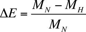
where M_H and M_N denote the average cancer mortality among people with higher and lower education, respectively. Basing on the data from 2002 (Wojtyniak and Goryński 2008) one can find the result of eqn (9) as ΔE ≈ 0.12.

The final form of CMR's correction factor connected with education is given as:

C O R R_{C M R} [%] = Δ E (F_{H B} - F_{L B})

(10)

Formula (10) means that the 1% excess of people with higher education results in a decrease of CMR by 0.12%.

Economic status

There are two different information about economical factors in Table 3: administrative budget per capita and real personal income (only for sets 1–3). Because of partial data of the latter, the administrative expenditure can be only taken as a real inhabitants’ economic status (connected for example with medical standards). Taking B_HB and B_LB as regional budgets (Table 3) one can find the relative difference in expenditure as:

Δ B = \frac{B_{H B} - B_{L B}}{B_{H B}}

(11)

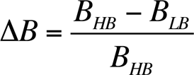
Formula (11) is useful to find the final correction factor connected with the budget per capita as:

C O R R_{C M R} [%] = Δ R \cdot Δ B

(12)

where ΔR is again just assumed to be not larger than 1.5%.

Environmental pollution

Data about environmental pollution are presented in Table 3 as dust in air, gas in air and pollution in water (without set 6). The average pollution in air [kg/year] can be assumed as:

Z = w \cdot P_{d u s t} + (1 - w) \cdot P_{g a s}

(13)

where P_dust and P_gas are the values of air pollution (from Table 3) and their weight assumed to be w = 0.8.

The relative ratio for comparing the Z (13) in HB and LB areas can be assumed as:

Δ Z = \frac{Z_{L B} - Z_{H B}}{Z_{H B}}

(14)

Basing on (14) one can find the correction factor as:

C O R R_{C M R} [%] = Δ Z \cdot Δ R

(15)

where ΔR is again assumed to be not larger than 0.02%.

Summary of confounding factors

In presented study only six confounding factors were taken into account: personal age, smoking, unemployment, education, economic status and air pollution. The calculated corrections of CMRs as well as the new simply adjusted results are presented in Table 4. One can note that data for sets 4–6 can be biased because of the lack of non-smokers statistics at the level of single counties. The results of relative risk for all cancers deaths are presented in Fig. 4 and for lung cancers only in Fig. 5. The RR uncertainties were assumed to increase by a factor of 50% because of potential uncertainties of overall adjustment.

The regression fit to RR (see Table 4 and Figs 4–5) results in a decrease of all cancer mortality by 1.17%/mSv/year (p = 0.02; χ² = 6.3) and by 0.82%/mSv/year (p = 0.2; χ² = 1.7) for lung cancer only. All fitting parameters are presented in Table 5.

DISCUSSION

Ionizing radiation can cause cellular damages in organisms. In some cases such damages may be transformed to cancer (Lehnert 2007). The problem of an influence of low doses of radiation, similar to background levels, is still under debate, and this is the reason why studies of correlation between natural radiation levels and cancer cases are important.

The topic of high-background radiation areas (HBRA) is considered in a number of studies (Wei et al. 1997; Jaworowski 2001; Hendry et al. 2009). One of the most popular data are based on cancer registry from Jangjiang in China (Wei and Sugahara 2000), Kerala in India (Nair et al. 1999), Guarapari in Brasil (Veiga and Koifman 2005), Ramsar in Iran (Monfared et al. 2006) or some areas of United States (Frigerio and Stowe 1975; Hart 2010, 2011a, 2011b; Bogen 1999; Bogen 2001; Bogen and Cullen 2002). Almost all of presented HBRA studies show decrease of cancer incidences or mortalities. Similar results are presented in this paper.

The paper shows results of the ecological analysis of six different cases in which the correlation between the level of natural radiation and cancer mortality was found. Every case concerns different size of analyzed area: from the biggest one (group of voivodeships) to the smallest one (a single county). All ecological studies, including presented one, contain bias connected with so called ecological fallacy (Bogen and Cullen 2002). Unfortunatelly the nature of ecological design makes mathematical impossibility of correcting it, because there are no data on individual relationships between inhabitants. In that way the presented study can not be free from this problem (Seiler and Alvarez 2000). However, it was attempted to make corrections everywhere where this was possible.

In the case of data set 1 there are five South-located voivodeships placed in higher radiation level group, whereas the low radiation group of voivodeships is located on the West-Nord part of Poland (Fig. 1). The first group of voivodeships is highly industrial region, especially Silesia region (Dolnoślaͅskie, Opolskie and Ślaͅskie voivodeships), which could rather increase than decrease the cancer mortality. There are also topographical differences between both group: south voivodeships contains low mountains, where west-nord are completely flat with Baltic Sea on the nord coast.

The data set 2 is similar to set 1.

In the case of data set 3 one can find the Małopolskie voivodeship (called also Małopolska province), which is rather upland region with Tatra mountains on the south. The biggest city is Kraków (Cracow) with a population about 760 000. There is no heavy industry situated outside the city. The Zachodniopomorskie voivodeship (called also Pomorze Zachodnie province) is seaboard region with the Baltic sea coast on the nord. The biggest city is Szczecin (Stettin) with a population about 410 000. The only heavy industry is situated in the city (international seaport).

In the case of data sets 4 and 5 the high radiation counties are located in the mountains (Tatra and Sudetes), whereas low radiation counties are located on flat area in the western Poland. There is no heavy industry in the analyzed counties. All analyzed counties are parts of voivodeships from set 2 (Fig. 2).

In the case of data set 6 there are two cities, which are simultaneously counties: Jelenia Góra located in Sudetes mountains and Świnoujście located on Baltic sea coast on three islands. The difference between elevations above mean sea level equals 342 meters (Table 1).

As the unadjusted data show, there is consistent trend showing a decrease of the RR for cancer deaths with an increase of the natural background radiation level (Table 2). Obviously, one can seek explanations of the effect in differences in medical care, geographical influences, industry, migration of population etc. However, the simple adjustment of data (Tables 3 and 4) shows also the same trend of cancer risk as unadjusted ones (Figs 4 and 5).

The presented calculations for adjustment are basing on six confounding factors: average age (eqn (5)), smoking (eqn (7)), unemployment (eqn (8)), education (eqn (10)), budget per capita (eqn (12)) and air pollution (eqn (15)). Table 3 shows that the differences in all confounding factors for sets 1–3 are rather small. One can thus conclude that all six correction factors (Table 4) have rather weak influence on the final results. This is not the case of sets 4–6, where huge differences of values gathered in Table 3 (e.g. budget per capita or environmental pollution) are observed. In this case the calculations based on eqns (5), (7), (8), (10), (12) and (15) can strongly change final values of last three points in Figs 4 and 5. The only conclusion is that one has to be very careful when using specific calculations and values of confounding factors listed in Table 3. As it was mentioned in previous section, the results for sets 4–6 can be additionally biased because of the smoking statistics not precisely known for single counties.

As it was explained earlier, the original CMR values (Table 2) are not age-adjusted. The information about age-adjusted cancer mortality is available in National Cancer Registry (KRN 2011) only for voivodeships (sets 1–3). Fig. 6 thus contains the unadjusted (Table 2), age-adjusted (KRN 2011) and adjusted (Table 4) relative risks for sets 1–3. One can observe the differences in these three types of data.

FIGURE 6.

The relative risk of all cancer death in sets 1–3 using unadjusted (Tab. 2), age-adjusted (KRN 2011) and adjusted (Tab. 4) data. ^∗p < 0.05

Figs 4 and 5 show the final results of the presented analysis: the average cancer mortality for all cancers (Fig. 4) and for lung cancers only (Fig. 5). The cited figures contain both adjusted (square points) and unadjusted (circle points) results. One can easily see that all results show the same trend, irrespective of which data (adjusted or unadjusted) were taken into consideration. The large uncertainties and p-values of adjusted results suggest that the statistical significance of presented trends is rather small (Table 5). Consequently, the valid question is whether the observed decrease of mortality is solely due to the level of ionizing radiation.

Many studies show that some doses of ionizing radiation can decrease number of cancers in the population (Sanders 2010). The possible radiation hormetic effect is connected with adaptive response of the humans’ immune system which is activated to better care and repair of DNA damages (Feinendegen et al. 2000; Calabrese and Baldwin 2002; Luckey 2006). The data presented in this paper show that the observed dose-effect relationship may be due to radiation hormesis.

Footnotes

ACKNOWLEDGEMENTS

The authors wish to express their gratitude to Chief Inspectorate of Environmental Protection (Poland) for a detailed radiological data from State Environmental Monitoring, as well as to Krzysztof Isajenko and Kalina Mamont-Cieśla from Central Laboratory for Radiological Protection.

The research was supported by European Union as a part of European Social Fund (PO KL 2007–2013, priority VIII, subaction 8.2.2 Regional Strategies of Innovation, “Potencjał naukowy wsparciem dla gospodarki Mazowsza – stypendia dla doktorantów“).

1

“voivodeship” is an official English translation of Polish word “województwo”, which is similar to the meaning of “province”; see: .

2

there are two different Krośnieński counties in Poland: first (taken into the analysis) in Lubuskie voivodeship, and the second in Podkarpackie voivodeship.

3

both sources contain data on popular radioisotopes concentration and gamma rays dose-rates in about 19 500 measurement points in Poland. The data do not characterize inter-individual variability among levels of individual exposure experienced within each geographic region.

4

in principle, the definition of CMR could be different. For example number of cancer deaths (from 1999 to 2009) could be divided by total population (or even e.g. 100 000 inhabitants). However, in the present studies such value is given for the year 2009 only. In order to use such definition, it would be necessary to summarize the population value from 1999 to 2009. Then, a great bias would appear in CMR because of multiple use of same persons (e.g. the inhabitant lived in 1999 usually still live in 2000 etc.; however, people died in 1999 will not die once again). In that reason the CMR definition was choosen as a number of cancer deaths divided by a number of all deaths ratio.

5

the 68% confidence interval is identical with one standard deviation σ under the assumpion of normal distribution of measured values. To increase confidence interval up to 95% one can take two standard deviations (2σ) and double all ranges of uncertainties (e.g. in Figs 3–). The one standard deviation is usually used as a standard uncertainty measurement by physicists.

6

chi-squared function value corresponding to the goodness of fit. The p-value is the probability of obtaining a test statistic at least as extreme as the one that was actually observed, assuming that the null hypothesis is true (in this case RR=100% what means no effect).

7

there are two types of an official residence place in Poland. One is a place where somebody actually stays/lives and the second is his registered permanent residency. Usually both places are identical, but they also can be different, e.g. after short migration. The official statistics (including cancers) are basing on this second type only.

References

AGP (Atlas Geochemiczny Polski, Geochemical Atlas of Poland). 1995. Państwowy Instytut Geologiczny (Polish Geological Institute), Warszawa, Poland.

Bogen

K.T

. 1999. Lung Cancer Risk of Low-Level Exposures to Alpha Emitters: Critical Reappraisal and Experiments Based on a New Cytodynamic Model. Final Report on LDRD Project 97-ERD-050, Lawrence Livermore National Laboratory, University of California.

Bogen

K.T

. 2001. Biologically based prediction of empirical nonlinearity in lung cancer risk vs. residential/occupational radon exposure. Hum Ecol Risk Assess 7:811–827.

Bogen

K.T.

Cullen

. 2002. Residential radon in U.S. counties vs. lung cancer in women who predominantly never smoked. Environ Geochem Health 24:229–247.

Calabrese

E.J.

Baldwin

L.A

. 2002. Radiation Hormesis and Cancer. Human & Ecological Risk Assessment, vol. 8, no. 2.

Cohen

B.L

. 2000. Updates and extensions to tests of the linear-no threshold theory. Technology, vol. 7: 657–672.

Feinendegen

L.E.

Bond

V.P.

Soudhaus

C.A

. 2000. The dual response to low-dose irradiation: induction vs. prevention of DNA damage. In: Yamada

Mothersill

Michael

Potten

(eds), Biological Effects of Low Dose Radiation, pp. 3–17. International Congress Series 1211, Elsevier Science, Amsterdam.

Fornalski

K.W.

Dobrzyński

. 2011. Pooled Bayesian analysis of twenty-eight studies on radon induced lung cancers. Health Physics 101(3): 265–273.

Frigerio

N.A

Stowe

R.S

. 1975. Carcinogenic and genetic hazard from background radiation. In: Symposium on Biological Effects of Low-Level Radiation Pertinent to Protection of Man and His Environment, Chicago, IL, IAEA-SM-202/805, Vol. 2, pp. 385–393. International Atomic Energy Agency, Vienna, Austria.

10.

GUS (Główny Urząd Statystyczny, Central Statistical Office). 2007. Ochrona środowiska (Environment). Warszawa, Poland.

11.

GUS (Główny Urząd Statystyczny, Central Statistical Office). 2011. Cancer statistics. Available at: www.stat.gov.pl.

12.

Hart

. 2010. Mean cancer mortality rates in low versus high elevation counties in Texas. Dose Response 8: 448–455.

13.

Hart

. 2011a. Cancer mortality for a single race in low versus high elevation counties in the U.S. Dose-Response 9: 348–355.

14.

Hart

. 2011b. Lung cancer in Oregon. Dose Response 9(3): 410–415.

15.

Hendry

J.H.

Simon

S.L.

Wójcik

Sohrabi

Burkart

Cardis

Laurier

Tirmarche

Hayata

. 2009. Human exposure to high natural background radiation: what can it teach us about radiation risks?. J. Radiol. Prot. 29: A29–A42.

16.

Jaworowski

. 2001. Ionizing radiation in the 20th century and beyond. Symposium Entwicklungen im Strahleschutz, Munich, November 29. Available at: www.cns-snc.ca/branches/Toronto/radiation.

17.

KRN (Krajowy Rejestr Nowotworów, National Cancer Registry). 2011. Cancer database. Available at: http://85.128.14.124/krn/.

18.

Lehnert

. 2007. Biomolecular action of ionizing radiation. Taylor & Francis, New York – London.

19.

Luckey

T.D

. 2006. Radiation hormesis: the good, the bad and the ugly. Dose-Response 4(3): 169–190.

20.

Monfared

A.S.

Jalail

Sedaghat

. 2006. High natural background radiation areas in Ramsar, Iran: can inhabitants feel safe?. Int. J. Low Radiat. 3: 20–27.

21.

MRP (Mapy Radioekologiczne Polski, Radioecological Maps of Poland). 1995. Państwowy Instytut Geologiczny (Polish Geological Institute), Warszawa, Poland.

22.

Nair

Nambi

K.S.V.

Amma

N.S

. 1999. Population study in the high natural background radiation area in Kerala, India. Radiation Research 152: S145–S148.

23.

RAP (Radiologiczny Atlas Polski, Radiation Atlas of Poland). 2005. Centralne Laboratorium Ochrony Radiologicznej (Central Laboratory for Radiological Protection), Warszawa, Poland.

24.

Sanders

C.L

. 2010. Radiation Hormesis and the Linear-No-Threshold Assumption. Springer, Heidelberg.

25.

Seiler

F.A.

Alvarez

J.L

. 2000. Is the “ecological fallacy” a fallacy?. Human and Ecological Risk Assessment 6(6): 921–941.

26.

UNSCEAR (United Nations Scientific Committee on the Effects of Atomic Radiation) Report 2006. Vol. II, Annex E. Sources-to-effect assessment for radon in homes and workplaces.

27.

Veiga

L.H.S.

Koifman

. 2005. Pattern of cancer mortality in some Brazilian HBRAs. Int Congress Ser 1276: 110–113.

28.

Wei

Sugahara

. 2000. An introductory overview of the epidemiological study on the population at the high background radiation areas in Yangjiang, China. J. Radiat. Res. (Tokyo) 41 (Suppl.): 1–7.

29.

Wei

Sugahara

Tao

. 1997. High levels of natural radiation, radiation dose and health effects (Chapter: High background radiation area – an important source of exploring the health effects of low dose ionizing radiation). Elsevier, Amsterdam.

30.

Wojtyniak

Goryński

(eds). 2008. Sytuacja zdrowotna ludności Polski (The health of citizens of Poland). Narodowy Instytut Zdrowia Publicznego – Państwowy Zaklad Higieny (National Institute of Public Health - National Institute of Hygiene), Warszawa, Poland.

The Cancer Mortality in High Natural Radiation Areas in Poland

Abstract

Keywords

INTRODUCTION

SOURCES AND METHODS

UNADJUSTED RESULTS

Set 1 – two groups of voivodeships

Set 2 – two pairs of voivodeships

Set 3 – two voivodeships

Set 4 – two groups of counties

Set 5 – two pairs of counties

Set 6 – two counties

Summary of the unadjusted results

ADJUSTED RESULTS

Inhabitants’ age

Smoking

Migration

Unemployment

Education

Economic status

Environmental pollution

Summary of confounding factors

DISCUSSION

Footnotes

ACKNOWLEDGEMENTS

1

2

3

4

5

6

7

References