Sage Journals: Discover world-class research

Abstract

A stochastic model based on the Markov Chain Monte Carlo process is used to describe responses to ionizing radiation in a group of cells. The results show that where multiple relationships linearly depending on the dose are introduced, the overall reaction shows a threshold, and, generally, a non-linear response. Such phenomena have been observed and reported in a number of papers. The present model permits the inclusion of adaptive responses and bystander effects that can lead to hormetic effects. In addition, the model allows for incorporating various time-dependent phenomena. Essentially, all known biological effects can be reproduced using the proposed model.

Keywords

Markov process Monte Carlo hormesis low-level radiation radiation threshold dose response model

INTRODUCTION

To date, a number of models of cellular responses to ionizing radiation have been published (UNSCEAR 1986; Calabrese and Baldwin 2003; Feinendegen 2005; Scott et al. 2007; Leonard 2008). Although the notion of probability of a given process is often used, most of the models demonstrate a rather deterministic approach resulting in more or less complicated mathematical formulas describing the biology of the cell and the physics of the radiation. Usually, the analytical formulas intend to show specific biological reactions of a cell culture or an organism in terms of probabilities and their distribution. However, at the very end, an analytical formula is used and the stochasticity of the processes is not obvious.

A relevant mathematical model should account for all variants of biological phenomena such as bystander effects (Prise et al. 2003; Leonard 2008), adaptive responses (Feinendegen et al. 2000), radiosensitivity, probability of natural death, cellular multiplication and mutation, and many others (ICRU 1983; Feinendegen and Pollycove 2001; Pollycove and Feinendegen 2003; Feinendegen and Neuman 2005; Lehnert 2007; Leonard 2008). This paper displays the results of simulations of possible outcomes of the exposure of cells to ionizing radiation. The simulations have been carried out within the framework of the Markov process.

METHODOLOGY

A stochastic Markov process, or memorylessness, is one for which “the present state of the system is independent of its previous states” (Encyclopaedia Britannica 2011). Hence, the conditional probability distribution of the future states depends solely upon the present state (Booth 1967; Podgórska et al. 2002; Trivedi 2002).

The reaction of a simulated simple organism (i.e., a group of cells) to ionizing radiation is analyzed in two numerical loops (see Fig. 1). Every step within the first loop represents the actual state of the cells. One can view the steps in this loop as the units of time. At each step, the cells may be growing old exhibiting the possibly altered states or those newly formed by the division of one or more progenitors. All these states are created in the second loop which inspects and acts on the set of cells delivered by the previous step. The second loop takes the cell one by one and uses a stochastic tree of probabilities which alter the state of the cell depending on whether it has been irradiated or not, has become mutated, cancerous, dead, etc. In this way, a new state of cells is created and the process reiterates in the next step, i.e. returns to the first loop.

FIG. 1.

General idea of the model: two loops over the steps and the cells.

The presented numerical loops contain the trees of probabilities, so purely mathematical values of these probabilities are intended to describe the biology of the cells (Lehnert 2007; ICRU 1983). An example of how the developed algorithm works is shown in Fig. 1 where the arrows displayed are just randomly selected for demonstration. A detailed presentation of the probability tree can be found in other figures. Since the primary aim of this paper is to show how such a type of the model works, some advanced biological mechanisms have not been considered here – they will be dealt with in the future calculations.

All the described rules work for the determined and constant value of dose per step: D. A change in D means that the calculations must start from the beginning. The total absorbed dose is a product of D multiplied by the number of steps K. Consistently, the dose D shown in all the figures is the dose per unit time and not the total dose which has led to the observed effect.

Construction of the stochastic tree of probabilities is the most important part of the model's algorithm (Booth 1967). The tree consists of a dozen of input parameters, e.g. the values of probabilities or the typically assumed constants.

The model presented in this paper shows a new method of simulation of a cellular response to an absorbed dose of radiation. The results demonstrate that, by using a given set of parameters, all the known reactions can be modeled. Currently, however, it is inherently difficult to find values of the probabilities which are closest to reality.

THE ALGORITHM

The numerical algorithm begins with setting a population of N cells. At first, all of the cells are “healthy“. At each (time) step, a stochastic tree of possibilities is applied to every i-th cell (see Fig. 2). Generally, the cell can be healthy, mutated, or cancerous. By definition, a healthy cell does not contain mutations and a mutated cell contains one or more mutations. However, not every cell that has been hit by radiation will develop a mutation. This process is regulated by the appropriate probability of mutation. A cancer cell is one transformed under certain conditions from a mutated cell, assuming that at least three genetic mutations have occurred (Hahn et al. 1999).

Every healthy, mutated, or cancerous cell can be irradiated (hit) with the probability P_hit (Bryszewska and Leyko 1997; Simmons and Watt 1999):

P_{h i t} = 1 - e x p (- c o n s t_{1} \cdot D)

(1)

where D denotes, as explained earlier, a dose per single cell in one simulation step, and const₁ is a scaling constant. In other words, P_hit is the probability of hitting a cell by radiation. The formula (1) is chosen just to describe a typical linear or quadratic dependence in the low-dose region and to make sure that the cell is hit at a very high dose per step. Obviously, one could use e.g. a stretched exponential or many other formulas as well. The choice of (1) is probably the simplest one (Bryszewska and Leyko 1997; Simmons and Watt 1999). For applications such as the one used herein, one is practically operating in the low dose region where eq. (1) is well approximated by a linear function of the dose. This equation can reflect the notion of cross section used, e.g. in particle physics.

FIG. 2.

First part of the stochastic tree for each cell. See text and Figs 3 to 8 for more details.

The algorithm works based on the random numbers generator¹ which determines all the probabilities. Each probability is drawn and is assigned a random value from 0 to 1. Depending on the generated value, a given branch of the tree is chosen.

Within the first part of the stochastic tree (see Fig. 2) six scenarios are possible, each of them serving as a starting point for the following stages, as shown in Figures 3 through 8.

1. A healthy cell has been hit by radiation (Fig. 3).

There are seven possible consequences of hitting a healthy cell (Fig. 3), that is, the cell can:

FIG. 3.

A portion of the stochastic tree from Fig. 2 – a healthy cell has been hit.

naturally die (probability P_D );

be killed by a single hit (probability P_RD );

spontaneously mutate, irrespectively of the hit (probability P_M );

naturally multiply (probability P_S );

generate bystander signals to the nearby cells (probability P_B );

become mutated by radiation (probability P_RM );

stay intact (probability 1-P_D-P_RD-P_S-P_M-P_B-P_RM ).

The term “probability of natural cell death” (P_D ), as used throughout, is a rather broad one. Death can be executed by two major mechanisms: apoptosis or necrosis. In order to keep the algorithm as simple as possible, we have used a single constant value of probability P_D.

Probability of the immediate cell death as a result of a precise, single hit by radiation, P_RD , is assumed to be linearly dependent upon dose per step D with a scaling factor const₂ :

P_{R D} = c o n s t_{2} \cdot D

(2)

Eq. (2) must be constrained by the natural condition valid for all the probabilities, namely: P_RD ≤ 1. When a cell becomes mutated, either spontaneously (P_M ) or by radiation (P_RM ), its status changes from “healthy” to “mutated“. In this case the number of mutations in the cell is one. Generally, cells can harbor more than one mutation. The value of P_RM is again assumed to be a linear function of the dose per step, D:

P_{R M} = c o n s t_{3} \cdot D a n d P_{R M} \leq 1

(3)

where const₃ is yet another scaling constant. The linear relationships (2) and (3) are selected for simplicity only, and can, if necessary, be replaced by any other form.

It has been shown in experimental kinetic analyses of human cell cultures that four to seven rate-limiting stochastic events – thought to be distinct somatic mutations and the triggered cellular signaling pathways thereof – are required for the formation of a tumorigenic cell (Renan 1993; Hahn et al. 1999; Hahn and Weinberg 2002). Based on this assumption, one can model the probability of transformation of a mutated cell into a cancerous cell using e.g. the following set of equations:

{\begin{array}{l} P_{R C} = c o n s t_{4} \cdot Q w h e n Q i s l e s s t h a n 4 \\ P_{R C} = 0.1 \cdot Q w h e n Q i s m o r e t h a n 3 a n d l e s s t h a n 11 \\ P_{R C} = 1 w h e n Q i s m o r e t h a n 10 \end{array}

(4)

where Q is the number of mutations in the investigated cell. The value of 1-P_RC describes the probability that the mutations generated in the cell will not result in tumorigenic transformation. Model (4) can be replaced by a continuous one once biological mechanisms of such a transformation are better understood.

One possible cause of mutations in cells that are in the vicinity of a hit cell is a bystander effect (with the probability P_B ). The algorithm selects randomly one nearby cell from the investigated i'th cell. When the neighboring cell is healthy its status will change from “healthy” to “mutated” (assuming one mutation in the cell). The number of mutations in this nearby cell increases by 1 if the cell has already contained mutations. The investigated i'th cell preserves its status (and the number of mutations). The probability of the bystander effect, P_B , is given by any probability distribution function with the maximum value at low doses (Feinendegen 2005). Four examples of such possible distributions (described by appropriate polynomials) are shown in Fig. 9.

Notably, in this approach we have assumed that the bystander effect causes only adverse outcomes and its possible beneficial effects (Prise et al. 2003; Leonard 2008; Mothersill and Seymour 2006) have been ignored. Within the present context of the algorithm a positive result would enhance the branch of the adaptive response. Again, for the sake of simplicity, such a possibility as well as an adaptive response limiting the number of non-radiogenic mutations has been excluded from the modeling.

2. A healthy cell has not been hit (Fig. 4).

There are four possible consequences of the case when a healthy cell has not been hit by radiation (Fig. 4):

the cell naturally dies (probability P_D );

the cell spontaneously mutates (probability P_M );

the cell naturally multiplies (probability P_S );

nothing happens (probability 1-P_D-P_S-P_M ).

FIG. 4.

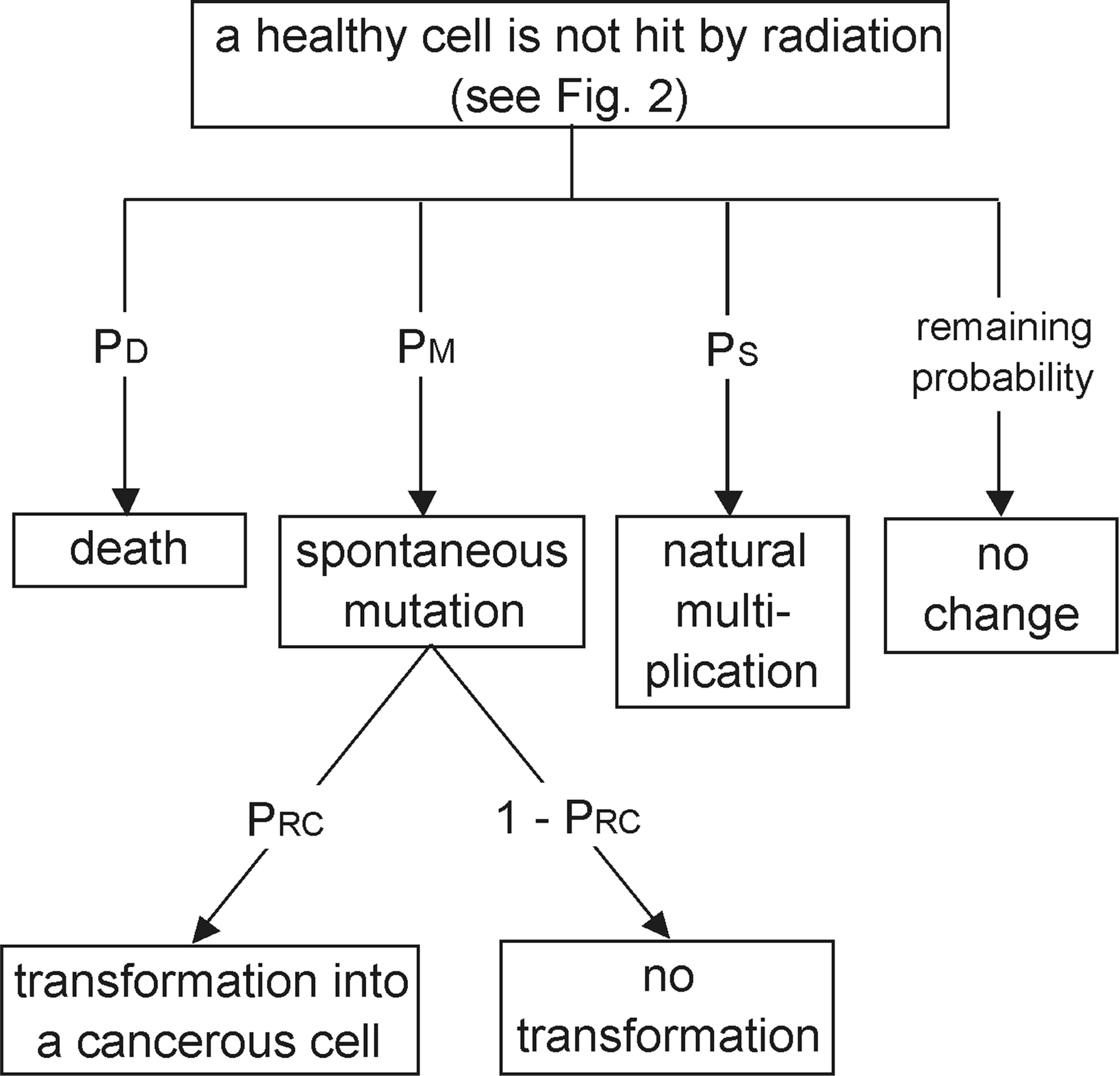
A portion of the stochastic tree from Fig. 2 – a healthy cell has not been hit.

As in section (1), the mutated cell can change into a cancer cell with the probability P_RC

In this case, bystander effects may also be produced by non-hit cells which exhibit, for example, enhanced oxidative metabolism. As mentioned above, such effects have not been accounted for in the present algorithm.

3. A mutated cell has been hit (Fig. 5).

In this case the mutated cell can behave in one of the following ways (Fig. 5):

it can naturally die (probability P_MD );

it can be killed by one precise hit of radiation (probability P_RD );

it can spontaneously mutate one more time (probability P_M );

it can naturally multiply (probability P_MS );

an adaptive response can be generated (probability P_A );

it can generate a bystander effect (probability P_B );

it can spontaneously repair one of the existing mutations (probability P_R );

it can be mutated by radiation (probability P_RM );

nothing happens (probability: 1-P_MD-P_RD-P_MS-P_M-P_A-P_B-P_R-P_RM ).

FIG. 5.

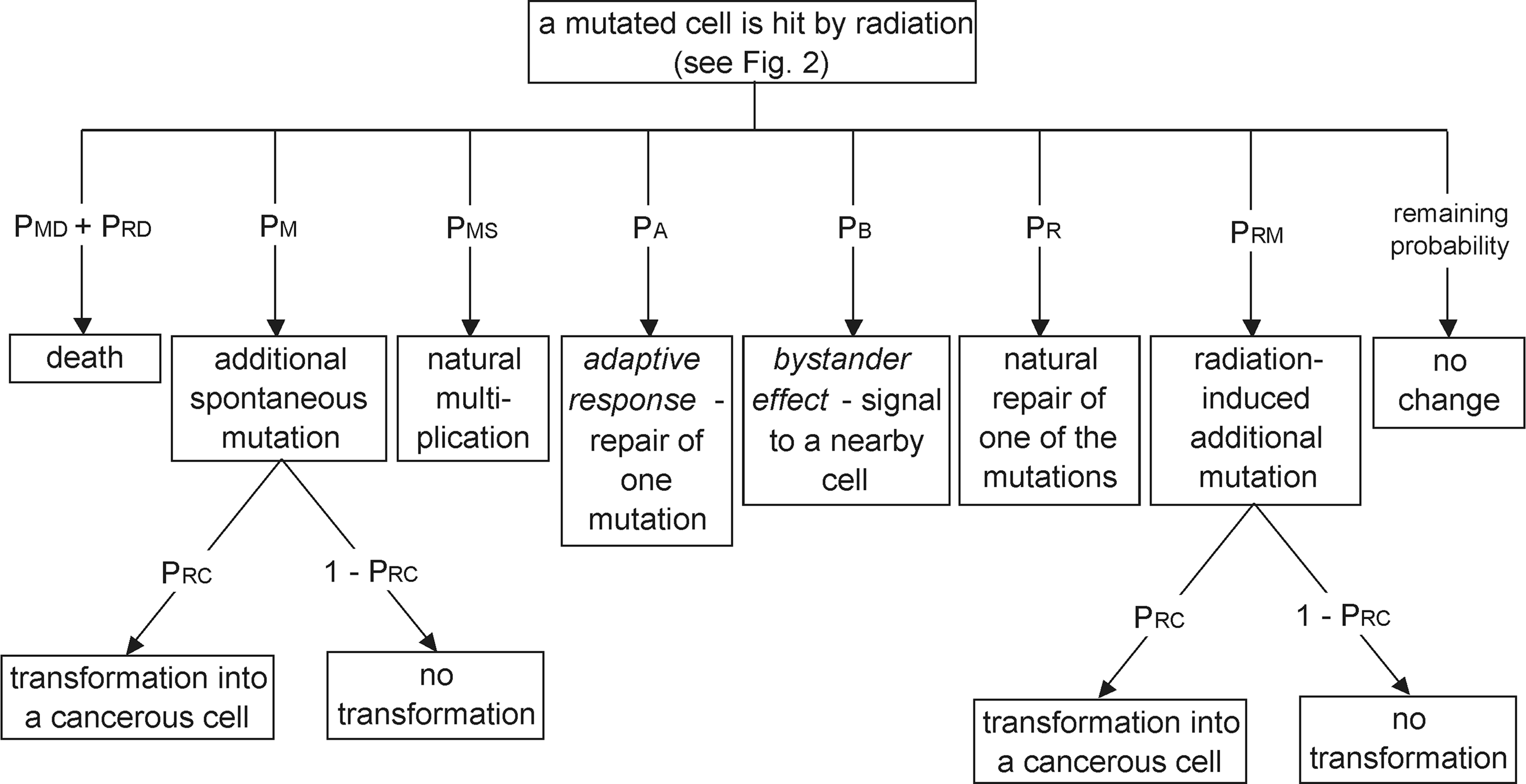
A portion of the stochastic tree from Fig. 2 – a mutated cell has been hit.

Generally, the probabilities P_MD and P_MS for mutated cells differ from the respective probabilities for healthy cells (P_D and P_S ). However, P_MS may create a progeny (daughter cell) with the same number of mutations.

The new probability P_A describes the adaptive response which is active only in mutated cells and reduces the number of mutations in the cell by 1. If the cell has only one mutation, its status will change from “mutated” to “healthy“. Probability of the adaptive response P_A is given by any probability distribution function with the maximum value at low doses (Feinendegen 2005). Four examples of such distributions (described by appropriate polynomials) are shown in Fig. 10.

In a manner comparable to those described in the previous sections the mutated cell, having sustained mutations with probabilities P_M and P_RM , can be transformed into a cancer cell with the probability P_RC.

4. A mutated cell has not been hit (Fig. 6).

There are six possible outcomes for a mutated cell that has not been hit (Fig. 6):

the cell naturally dies (probability P_MD );

the cell spontaneously mutates one more time (probability P_M );

the cell naturally multiplies (probability P_MS );

an adaptive response develops (probability P_A );

the cell naturally repairs one mutation (probability P_R );

there is no effect (probability: 1-P_MD-P_MS-P_M-P_A-P_R ).

FIG. 6.

A portion of the stochastic tree from Fig. 2 – a mutated cell has not been hit.

P_MS creates a progeny (daughter cell) with the same number of mutations. As indicated earlier, the cell mutated with the probability P_M can change into a cancer cell with the probability P_RC.

5. A cancer cell has been hit (Fig. 7).

When a cancer cell has been hit by radiation there are six possible consequences (Fig. 7), i.e.:

the cell naturally dies (probability P_CD );

the cell is killed by one precise-hit of radiation (probability P_RD );

the cell naturally multiplies (probability P_CS );

the cell dies because of the radiation-induced additional damage (probability P_CRD );

the cell generates a bystander effect (probability P_B );

nothing happens (probability: 1-P_CD-P_RD-P_CS-P_CRD-P_B ).

The probabilities P_CD and P_CS should be significantly different from P_MD and P_MS because of the different biology of the cancer cell. In order to make the model as simple as possible, it assumed that the probability that the cancer cell will die because of an extra hit (due to its radiosensitivity) changes linearly with the dose per step:

P_{C R D} = c o n s t_{5} \cdot D a n d P_{C R D} \leq 1

(5)

FIG. 7.

A portion of the stochastic tree from Fig. 2 – a cancer cell has been hit.

FIG. 8.

A portion of the stochastic tree from Fig. 2 – a cancer cell has not been hit.

6. A cancer cell has not been hit (Fig. 8).

When a cancer cell has not been hit, one of the following three situations (Fig. 8) can be expected:

the cell naturally dies (probability P_CD );

the cell naturally multiplies (probability P_CS );

nothing happens (probability: 1-P_CD-P_CS ).

SUMMARY OF THE INPUT PARAMETERS

The described algorithm contains a stochastic tree and dozens of input parameters – probabilities and constant factors. All of them, listed in Table 1, can be selected subjectively and their suggested values are important for the final result. These parameters describe, rather intuitively, biological and physical effects of the interaction of ionizing radiation with cells. In particular, one considers a special form (1) of the probability distribution for a cell being irradiated (P_hit ). Other probabilities, such as a cell developing a mutation (P_RM ) or getting killed because of its radiosensitivity or the precise hit (P_CRD and P_RD ), or even the probability that a mutated cell is transformed into a cancerous one (P_RC ) are assumed to vary linearly with the dose per step. There are also probabilities given by one simple constant value such as the probability that a healthy/mutated/cancer cell will naturally die (P_D / P_MD / P_CD ) or multiply (P_S / P_MS / P_CS ). The probability of a spontaneous mutation (P_M ) and a natural repair (P_R ) are also simple constants. In contrast, the bystander effect (P_B ) or adaptive response to radiation (P_A ) are given by certain dose dependent functions.

TABLE 1.

Summary of all the input parameters to the model presented in Figs 1–8.

Probability	Explanation
P_D	Probability that a healthy cell dies because of natural reasons
P_MD	Probability that a mutated cell dies because of natural reasons
P_CD	Probability that a cancer cell dies because of natural reasons
P_s	Probability that a healthy cell multiplies; the daughter cell is also healthy
P_MS	Probability that a mutated cell multiplies; the daughter cell is also mutated with the same number of mutations as the parent cell
P_CS	Probability that a cancer cell multiplies; the daughter cell is also tumorigenic
P_M	Probability of a spontaneous mutation in a cell – first in a healthy cell, and the following in a mutated one.
P_R	Probability of natural repair of one mutation in the mutated cell
P_B	Probability of a bystander effect given by the probability distribution (see Fig. 9); the irradiated cell (healthy, mutated or cancerous) sends a signal to neighbouring cells which results in a mutation in one of them
P_A	Probability of an adaptive response given by the probability distribution (see Fig. 10); the mutated cell repairs one mutation and if there are no other mutations, the “healthy” state of the cell is restored
P_hit	Probability that a cell is hit by a particle of radiation; this is associated with the constant factor const₁
P_RM	Linear probability that a mutation develops in the irradiated cell; for the healthy cell this will be the first mutation, for the mutated one – the following mutation; this probability is associated with the constant factor const₃
P_RC	Probability that the mutated cell is transformed into the cancerous one; this is associated with the constant factor const₄
P_RD	Probability that a cell dies from a precise hit by radiation; this is associated with the constant factor const₂
P_CRD	Probability that a cancer cell dies because of its specific radiosensitivity; this is associated with the constant factor const₅
D	Analysed value of the dose (in [mGy]) per one step of cells
K	Number of cell steps (usually equal to 300); the value of K·D refers to the cumulative dose
N	Number of cells in the first step (usually equal to 1000)

To cut off one of the branches in the stochastic tree (Figs 2–8) one can reduce the respective probability value to zero. It is also possible to modify the model by adding more branches of the tree representing the more detailed biophysical effects.

RESULTS

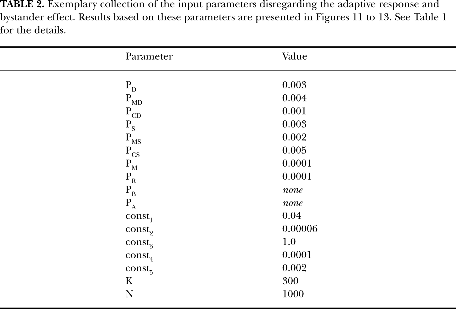
The present model can work with all values of the input parameters (Tab. 1), either intuitively assumed or precisely measured. Usually, it is difficult to obtain the precise data, because, in reality, there are many types of cells with different properties, age, etc. Sometimes, however, it is possible to draw more or less precise values of the parameters listed in Table 1. For example, in case of the parameter P_RD one can use const₂ ≈ 0.00006 (Feinendegen et al. 2010). Also, probability functions of the bystander effect (P_B ) and adaptive response (P_A ) can be taken as B1 and A1 (see Figs 9 and 10), respectively. Their forms correspond qualitatively with the ones found in the reference literature (Feinendegen 2005; Feinendegen et al. 2010).

One suggested collection of the parameters’ values is presented in Table 2. Results of the model based on the Table are shown in Figures 11 through 13.

FIG. 9.

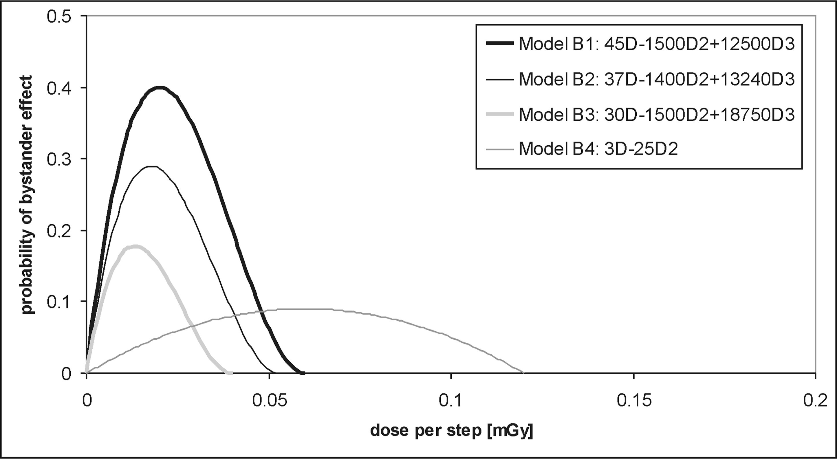
Four exemplary models (B1, B2, B3, B4) of the probability distribution of the bystander effect (P_B) described by up to the third-order polynomials. The labels “D2” and “D3” in the figure's legend stand for “D²” and “D³“, respectively, where D is the dose per one state (step) of cells

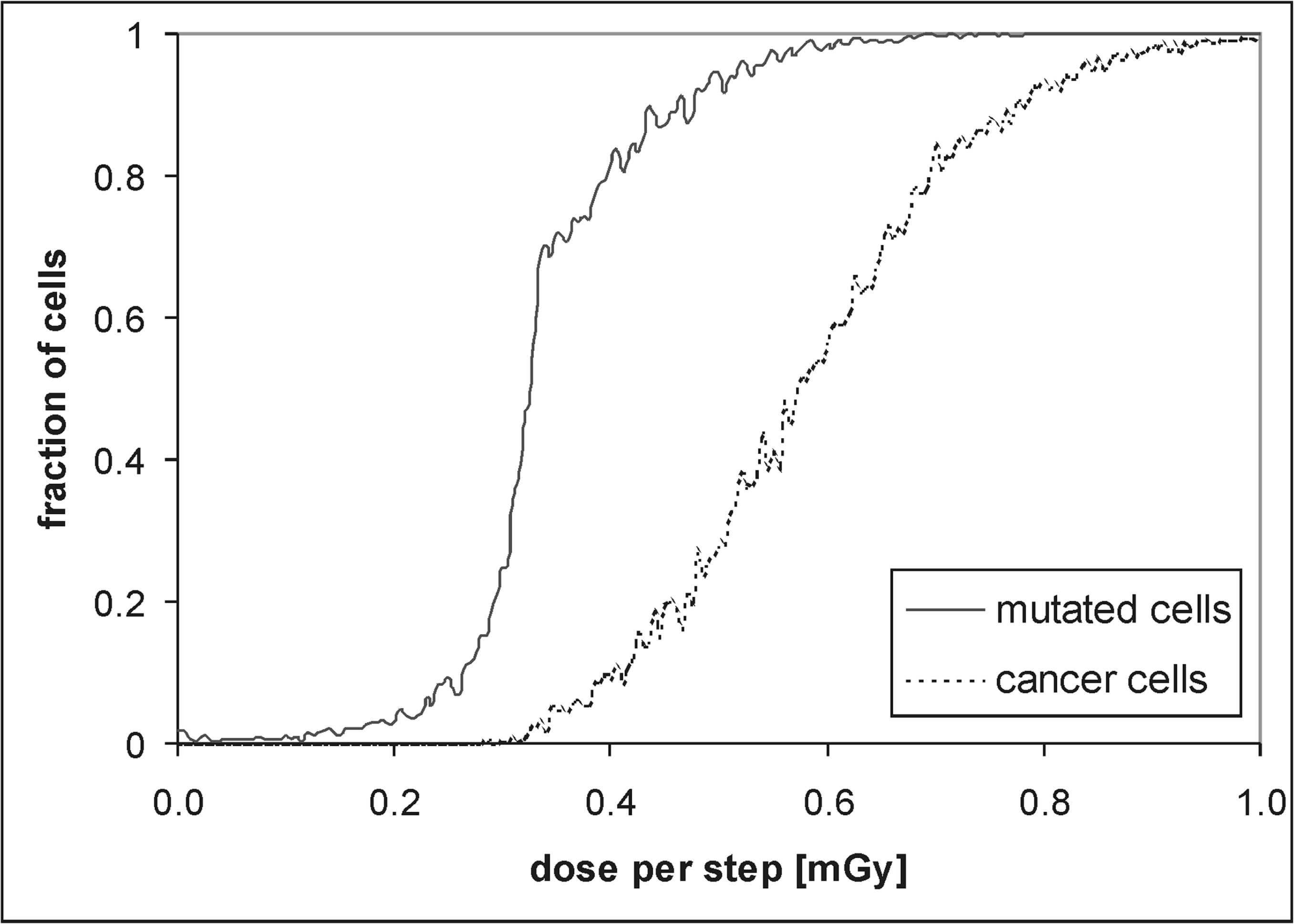
In Fig. 11 the relative ratios of the mutated (solid line) and cancer cells (dotted line) to all the cells are shown in cases when the adaptive response and bystander effect are not taken into account. As shown, the model assumes that approx. 3% of the cells are naturally mutated at the beginning, i.e., independently of any radiation (Fig. 11). The straight line can easily be drawn through most of the data showing the number of the mutated cells. In the case of cancer cells, however, one can observe clear threshold at the dose per step of approx. 0.2 mGy. Cancer cells are also treated as mutated ones. In Fig. 12 the same data obtained for the lowest doses per step are shown (D < 0.4 mGy): a threshold for the formation of cancer cells at about 0.2 mGy per step and a nearly constant value of the mutated cells below the dose of 0.04 mGy per step are clearly indicated. At the dose of about 0.7 mGy per step practically all the cells are mutated and neoplastically transformed. Fig. 13 shows that at this dose per step the total number of cancer cells increases substantially – it is more than twice as high as the initial number of the “healthy” cells. Notably, the average number of mutations per each cell approximates six. With the still increasing dose the probability of the cell's death overcomes the probability of its multiplication; therefore the number of mutations per cancer cell is decreasing (Fig. 13).

FIG. 10.

Four exemplary models (A1, A2, A3, A4) of the probability distribution of the adaptive response (P_A), described by up to the third-order polynomials. “D2” and “D3” in the figure's legend stand for “D²” and “D³“, respectively, where D is the dose per one state (step) of cells.

TABLE 2.

Exemplary collection of the input parameters disregarding the adaptive response and bystander effect. Results based on these parameters are presented in Figures 11 to 13. See Table 1 for the details.

Parameter	Value
P_D	0.003
P_MD	0.004
P_CD	0.001
P_S	0.003
P_MS	0.002
P_CS	0.005
P_M	0.0001
P_R	0.0001
P_B	none
P_A	none
const₁	0.04
const₂	0.00006
const₃	1.0
const₄	0.0001
const₅	0.002
K	300
N	1000

FIG. 11.

Results obtained with use of the set of parameters from Tab. 2. The fraction is shown of mutated (solid line) and cancer cells (dotted line).

FIG. 12.

Results obtained with use of the set of parameters from Tab. 2. The fraction is shown of mutated (solid line) and cancer cells (dotted line). The dose is limited to 0.4 mGy per step.

FIG. 13.

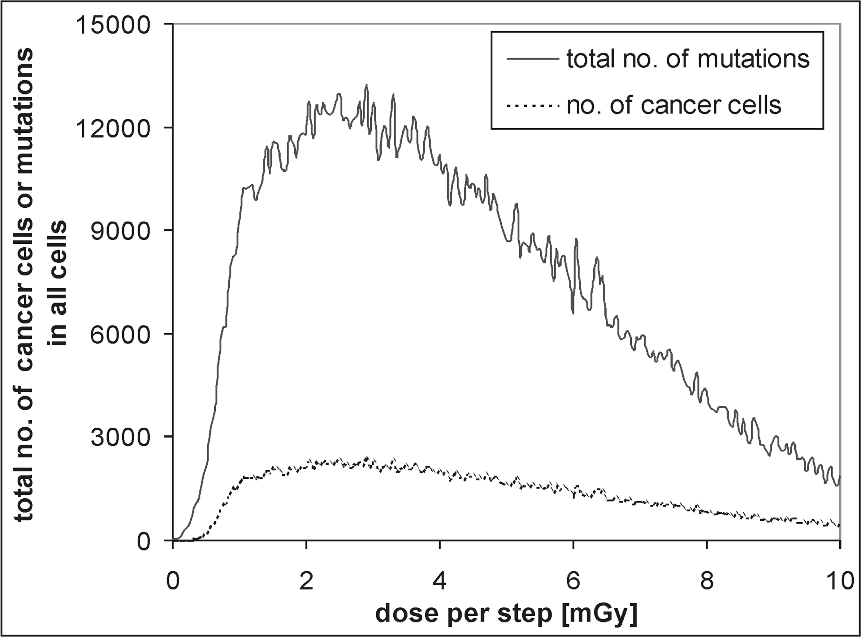
Results obtained with use of the set of parameters from Tab. 2. The total number is shown of mutations in all cells (solid line), along with the number of cancer cells (dotted line).

The results presented in Figures 11 through 13 do not include the adaptive response or the bystander effect. Figures 14 and 15 show the same results, but in this case P_A is taken as a model A1 = D – 5D ² + 6D ³ and P_B as a model B1 = 45D – 1500D ² + 12500D ³ (see Figures 9 and 10 for details). By comparing Fig. 15 with Fig. 12 one can note that when both the adaptive response and bystander effect are present a significant hormetic effect is manifested, especially below 0.15 mGy per step.

DISCUSSION AND CONCLUSIONS

The stochastic model used in the present paper most probably shows what can actually happen in a population of cells exposed to ionizing radiation. Such a stochastic approach seems to be better than many deterministic models because it takes into consideration some individual susceptibilities and probabilities rather than many phenomenological factors which, although called “probabilities” are not, in fact, used as such. In the present model, every run yields somewhat different results only because of the use of the truly probabilistic approach.

FIG. 14.

Results obtained with use of the set of parameters from Tab. 2 including the adaptive response and bystander effect. The fraction is shown of the mutated (solid line) and cancer cells (dotted line).

FIG. 15.

Results obtained with use of the set of parameters from Tab. 2 including the adaptive response and bystander effect. The fraction is shown of the mutated (solid line) and cancer cells (dotted line).

One of the advantages of using of a probability tree is a possibility of easily adding or cutting off some of its branches. The present algorithm has been significantly simplified in terms of its biological background, but it can certainly be further developed and made more complex in the future.

Based on the results presented in Figures 11 through 15, a number of conclusions can be drawn. Firstly, the observed fluctuations simply reflect the stochastic nature of the processes. Secondly, although most of the obtained relationships between the dose per step and the given outcome vary linearly with the dose (see Table 1), the final result is conditional upon the dose in a much more complicated way. Indeed, a clear-cut threshold for the development of cancerous cells can be seen regardless of whether or not any bystander effect or adaptive response has been accounted for (Figs 11 and 14). Thirdly, there is a diminution in the total number of mutations after absorption of a certain dose per step (Fig. 13), apparently, as a result of death of the cells exposed to a strong radiation field. Finally, when the bystander effect and adaptive response are taken into account, a significant hormetic effect can be seen in terms of the diminished number of the mutated cells (Fig. 15 versus Fig. 12) and a shift in the threshold for the appearance of cancer cells (Fig. 15).

In the present simulation an undefined cell culture with no association to any specific tissue has been used. Indeed, the present model has no ambition to develop the algorithm for more complex tissue reactions. However, a potential user of the model can take their own values of input parameters specifying the type of cells or the tissue they may want to investigate.

The obtained results are consistent with many epidemiological and experimental data demonstrating or implicating a threshold (Ullrich and Storer 1979; Miller et al. 1989; UNSCEAR 1986, 1994, 2000; Hosoi and Sakamoto 1993; Liu et al. 1996; Mitchel et al. 1999, 2003; Redpath et al. 2001, 2003; Ko et al. 2004, 2006; Elmore et al. 2005; Redpath and Elmore 2007; Nowosielska et al. 2008; Ulsh 2010). In particular, the specific shape of the dose-response relationship presented in Fig. 11 was recently demonstrated in the studies of death rates of the exposed laboratory rats and mice and the Chernobyl workers (Allison 2009; Henriksen and Maillie 2003; Zyuzikov et al. 2011). A similar shape is also presented in (Anderson and Storm 1992; UNSCEAR 1994), demonstrating a cumulative incidence of primary liver tumors among the Danish patients.

In turn, the shape of curves shown in Fig. 13 closely resembles the final cumulative rate of leukemia among mice (Di Majo et al. 1986; Robinson and Upton 1978; UNSCEAR 1986) and the absolute risk of breast cancer in women treated with radiotherapy (Shore et al. 1986; UNSCEAR 1994). Same shape of dose-effect relationship is seen in figure VI in (UNSCEAR 1994), where excess relative risk per sievert for mortality from leukemia of the life span study is presented. Finally, similar results were obtained by Shuryak et al. (2009) in their simulations of biological processes.

It must be stressed that the present model was not biased in any way towards a possibility of a threshold or hormesis. These effects seem to appear very naturally and, notably, the latter effect could be demonstrated only after taking the adaptive response into account. Obviously, the present model contains too many parameters to be readily adaptable to a particular situation. Nevertheless, one can easily control the influence of any of these parameters (processes) on the final result. The model can also be easily expanded to more sophisticated forms of the relationship between probabilities and doses.

The present approach may provide clues for modeling the impact of low doses on organisms with use of the Markov chain Monte Carlo techniques. A prospective user of the model can add new branches to the probability tree and/or can select a completely different set of the input probabilities. The values of such parameters listed in Table 2 are just an example of how the model can work. In order to describe a real biological system, the model will be further developed and elaborated in the future.

Footnotes

ACKNOWLEDGEMENTS

The authors wish to express their gratitude to Professor Zbigniew Jaworowski for his careful review of this paper and comments provided, as well as to Drs. Aneta Cheda, Ewa Nowosielska and Jolanta Wrembel-Wargocka for their valuable inputs.

1

The random number generator originates in the ROOT environment based on the C/C++ language; .

References

Allison

. 2009. Radiation and reason – the impact of science on a culture of fear. York.

Anderson

Storm

H.H

. 1992. Cancer incidence among Danish thorotrast-exposed patients. J. Natl. Cancer Inst. 84, pp. 1318–1325.

Booth

T. L

. 1967. Sequential Machines and Automata Theory (1st ed.). New York

Bryszewska

Leyko

. 1997. Biofizyka dla biologów ['Biophysics for biologists' – in Polish]. PWN, Warszawa.

Calabrese

E.J.

Baldwin

L.A

. 2003. The Hormetic Dose-Response Model Is More Common than the Threshold Model in Toxicology. Toxicological Sciences 71

Di Majo

Coppola

Rebessi

Bassani

Alati

Saran

Bangrazi

Covelli

. 1986. Dose-response relationship of radiation-induced Harderian gland tumours and myeloid leukaemia of the CBA/Cne mouse. J. Natl. Cancer Inst. 76, pp. 955–963.

Elmore

Lao

X-Y

Rightnar

Nelson

and Redpath

. 2005. Neoplastic transformation In vitro induced by low doses of 232 MeV protons. International Journal of Radiation Biology 81:291–297.

Encyclopaedia Britannica. 2011. www.britannica.com

Feinendegen

L.E

. 2005. Low doses of ionizing radiation: relationship between biological benefit and damage induction. A synapsis. World Journal of Nuclear Medicine 4

10.

Feinendegen

L.E.

Bond

V.P.

Soudhaus

C.A

. 2000. The dual response to low-dose irradiation: induction vs. prevention of DNA damage. Biol. Effects of Low Dose Radiation – Elsevier Science

11.

Feinendegen

L.E.

Neuman

R.D

. 2005. Physics must join with biology in better assessing risk from low-dose irradiation. Radiation Protection Dosimetry

12.

Feinendegen

L.E.

Pollycove

. 2001. Biologic responses to low doses of ionizing radiation: detriment versus hormesis. J. Nucl. Med. 42 (7 & 9).

13.

Feinendegen

L.E.

Pollycove

Neumann

R.D

. 2010. Low-dose cancer risk modeling must recognize up-regulation of protection. Dose-Response 8(2): 227–52

14.

Hahn

W.C.

Counter

C.M.

Lundberg

A.S.

Beijersbergen

R.L.

Brooks

M.W.

Weinberg

R.A.

. 1999. Creation of human tumour cells with defined genetic elements. Nature, 400: 464–468.

15.

Hahn

W.C.

Weinberg

R.A

. 2002. Rules for making human tumor cells. N. Engl. J. Med. 347: 1593–1603.

16.

Henriksen

Maillie

H.D

. 2003. Radiation & Health. Taylor & Francis.

17.

Hosoi

Sakamoto

. 1993. Suppressive effect of low dose total body irradiation on lung metastasis: dose dependency and effective period. Radiotherapy and Oncology 26:177–179.

18.

ICRU 1983. Microdosimetry. International Commission on Radiation Units and Measurements, Report No. 36.

19.

Lao

X-Y

Molloi

Elmore

and Redpath

. 2004. Neoplastic transformation in vitro following exposure to low doses of mammographic energy x-rays: Quantitative and mechanistic aspects. Radiation Research 162:646–654.

20.

Lao

X-Y

Kapadia

Elmore

and Redpath

. 2006. Neoplastic transformation in vitro: role of adaptive response and bystander effects. Mutation Research 597:11–17.

21.

Lehnert

. 2007. Biomolecular action of ionizing radiation. Taylor & Francis, New York – London.

22.

Leonard

B. E

. 2008. A review: development of a microdose model for analysis of adaptive response and bystander dose response behavior. Dose-Response, 6: 113–183

23.

Liu

Zhang

Liu

. 1996. Tymocyte apoptosis in response to low-dose radiation. Mutation Research 358:185–191.

24.

Miller

Howe

Sherman

Lindsay

Yaffe

Dinner

Risch

Preston

. 1989. Mortality from breast cancer after irradiation during fluoroscopic examination in patients being treated for tuberculosis. New England Journal of Medicine 321:1285–1289.

25.

Mitchel

REJ

Jackson

McCann

, and Boreham

. 1999. The adaptive response modifies latency for radiation-induced myeloid leukemia in CBA/H mice. Radiation Research 152:273–279.

26.

Mitchel

REJ

Jackson

Morrison

, and Carlisle

. 2003. Low doses of radiation increase the latency of spontaneous lymphomas and spinal osteosarcomas in cancer-prone, radiation sensitive Trp53 heterozygous mice. Radiation Research 159, pp. 320–327.

27.

Mothersill

Seymour

. 2006. Radiation-induced bystander effects: evidence for an adaptive response to low dose exposures?. Dose-Response 4(4), pp. 277–282.

28.

Nowosielska

E.M.

Cheda

Wrembel-Wargocka

Janiak

M.K

. 2008. Modulation of the growth of pulmonary tumour colonies in mice after single or fractionated low-level irradiations with X-rays. Nukleonika 53 (Suppl.1): S9–S15.

29.

Podgórska

. 2002. Markov chains in theory and applications (in Polish), Warszawa, Szkoła Główna Handlowa Oficyna Wydawnicza

30.

Pollycove

Feinendegen

L.E

. 2003. Radiation-induced versus endogeneous DNA damage. Human & Environmental Toxicology 22

31.

Prise

K.M.

Folkard

Michael

B.D

. 2003. A review of the bystander effect and ist implications for low-dose exposure. Radiation Protection Dosimetry Vol. 104, No. 4, pp. 347–355.

32.

Redpath

J.L.

Elmore

. 2007. Radiation-induced neoplastic transformation in vitro, hormesis and risk assessment. Dose-Response 5:123–130.

33.

Redpath

Liang

Taylor

Christie

, and Elmore

. 2001. The shape of the dose-response curve for radiation-induced neoplastic transformation in vitro: Evidence for an adaptive response against neoplastic transformation at low doses of low-LET radiation. Radiation Research 156:700–707.

34.

Redpath

Liao

X-Y

Molloi

, and Elmore

. 2003. Low doses of diagnostic energy x-rays protect against neoplastic transformation in vitro. International Journal of Radiation Biology 79:235–240.

35.

Renan

M.J

. 1993. How many mutations are required for tumorigenesis? Implications from human cancer data. Mol. Carcinogenesis 7: 139–146.

36.

Robinson

V.C.

Upton

A.C

. 1978. Competing-risk analysis of leukaemia and non-leukaemia mortality in X-irradiated male RF mice. J. Natl. Cancer Inst. 60, pp. 995–1007.

37.

Scott

B.R.

Haque

Palma

J.D

. 2007. Biological basis for radiation hormesis in mammalian cellular communities. Int. J. of Low Radiation 4/1

38.

Shore

R.E.

Hildreth

Woodard

Dvoretsky

Hempelmann

Pasternack

. 1986. Breast cancer among women given X-ray therapy for acute postpartum mastilis. J. Natl. Cancer Inst. 77, pp. 689–696.

39.

Shuryak

Hahnfeldt

Hlathy

Sachs

R. K.

Brenner

D. J

. 2009. A new view of radiation-induced cancer: integrating short- and long-term processes (Part I). Radiat. Environ. Biophys. (Springer).

40.

Simmons

J.A.

Watt

D.E

. 1999. Radiation Protection Dosimetry – a radical reappraisal. Medical Physics Publishing, Madison

41.

Trivedi

K. S

. 2002. Probability and Statistics with Reliability, Queueing, and Computer Science Applications, John Wiley & Sons, Inc.

New York

42.

Ullrich

and Storer

. 1979. Influence of irradiation on the development of neoplastic disease in mice. III. Dose-rate effects. Radiation Research 80:325–342.

43.

Ulsh

B. A

. 2010. Checking the foundation: recent radiobiology and the linear no-threshold theory. Health Physics 99(6): 747–758

44.

UNSCEAR 1986. Genetic and somatic effects of ionizing radiation. United Nations Scientific Committee on the Effects of Atomic Radiation 1986 Report to the General Assembly, with annexes. Annex B, part III and part IV, United Nations, New York, 1986

45.

UNSCEAR 1994. Sources and Effects of Ionizing Radiation. United Nations Scientific Committee on the Effects of Atomic Radiation 1994 Report to the General Assembly, with annexes. Annex A: Epidemiological studies of radiation carcinogenesis , United Nations, New York, 1994

46.

UNSCEAR 2000. Sources and Effects of Ionizing Radiation. United Nations Scientific Committee on the Effects of Atomic Radiation (Report to the General Assembly with Scientific Annexes) Annex I, United Nations, New York, 2000

47.

Zyuzikov

N. A.

Coates

P. J.

Parry

J. M.

Lorimore

S. A.

Wright

E. G

. 2011. Lack of nontargeted effects in murine bone marrow after low-dose in vivo X irradiation. Radiation Research 175, pp. 322–327

A Stochastic Markov Model of Cellular Response to Radiation

Abstract

Keywords

INTRODUCTION

METHODOLOGY

THE ALGORITHM

1. A healthy cell has been hit by radiation (Fig. 3).

2. A healthy cell has not been hit (Fig. 4).

3. A mutated cell has been hit (Fig. 5).

4. A mutated cell has not been hit (Fig. 6).

5. A cancer cell has been hit (Fig. 7).

6. A cancer cell has not been hit (Fig. 8).

SUMMARY OF THE INPUT PARAMETERS

RESULTS

DISCUSSION AND CONCLUSIONS

Footnotes

ACKNOWLEDGEMENTS

1

References