Are Some Neurons Hypersensitive to Metallic Nanoparticles?

Abstract

Engineered metallic nanomaterial particles (MENAP) represent a significant breakthrough in developing new products for use by consumers and industry. Skin application (e.g., via creams and sprays containing nanoparticles) may provide a key route of potential intake of MENAP and can lead to retrograde transport from nerve endings in the skin to the somatosensory neurons in dorsal root ganglia (DRG). This paper uses a novel theoretical model (stochastic threshold microdose [STM] model) to characterize survival of DRG neurons exposed in cell culture replicates to copper nanoparticles, based on published data. Cell death via autophagy is assumed here to occur as a result of the uptake (called hits) of the nanoparticles by mitochondria. Theoretical results are presented for the existence of a hypersensitive fraction (about 20%) of neurons that are killed in significant numbers when on average > 1 hit to the at-risk mitochondria occurs. Further, most hypersensitive neurons appear to be killed by a cumulative exposure of about 2,000 micromolar-hours and the remaining resistant cells may have dysfunctional mitochondria. Based on these theoretical findings, it is predicted that repeated exposure (e.g., over years) of the skin of humans to MENAP could lead to significant nervous system damage and related morbidity.

INTRODUCTION

Billions of dollars recently have been invested worldwide in nanotechnology research and development (Roco 2005). Metallic and other nanomaterials have properties that make them useful for many applications, including high conductivity material strengthening, increasing material durability, and altering material reactivity. Numerous nanomaterials are made of metals or metal oxides. The metals include iron, gold, zinc, silver, copper, lead, cerium, zirconium, cadmium, germanium, and selenium. Important engineered nanomaterials now in production includes metal oxides, fullerenes, carbon nanotubes, and quantum dots. Varieties of bio-nanotechnologies are being developed for biomedical applications. Nanoparticles also are being researched for possible use in cancer therapy (AshaRani et al. 2009); however, not very much is known about health risks to nanotechnology workers and the general public from nanoparticles (Donaldson et al. 2004; Hoet et al. 2004; Moghimi et al. 2005; Oberdörster et al. 2005; Powell and Kanarek 2006a, b; Hoover et al. 2007; Prabhu et al. 2009).

Nanoparticles typically are defined as engineered particles having at least one dimension <100 nanometers (nm). The particles could be inhaled, ingested, or enter the body via uptake through the skin (intact or wounded). Potential biological effects include DNA damage, mitochondrial damage, mutations, neoplastic transformation, cell killing, and related systemic effects (e.g., neurological dysfunctions, heart disease, and cancer).

The focus of the modeling in this paper is on insoluble engineered metallic nanomaterial particles (MENAP) made of copper and their cytotoxicity to dorsal root ganglia (DRG) in vitro. Copper nanoparticles are being manufactured for application in facial spray. Repeated application of such sprays over long periods could lead to the accumulation of a significant number of copper nanoparticles in nerve cells of the nervous system. Thus, it is important to conduct research related to assessing copper nanoparticle toxicity to neurons (Prabhu et al. 2009).

Copper is an essential trace mineral that plays an important role in energy production in the body's cells. High levels are found in the brain but are maintained in homeostasis because copper becomes toxic when in excess and not properly bound (Evans 1973; Sternleib 1980; Prabhu et al. 2009). Under toxic conditions, copper's redox reactivity can lead to the formation of reactive oxygen species (ROS) such as superoxide anion, hydrogen peroxide, and hydroxyl radical. Excess ROS can lead to cell damage through oxidative modifications of proteins, lipids, and nucleic acids, damaging their structures and functions (Halliwell and Gutteridge 1990; Galhardi et al. 2004; Prabhu et al. 2009).

Concern about the toxicity of copper has led to research in a variety of areas (Evans 1973; Nalbanadyan. 1983; Saris and Skulskii 1991; Pourahmad and O'Brien 2000; Cecconi et al. 2002; Gaetke and Chow 2003; Bertinato and L'Abbé 2004; Galhardi et al. 2004; Warheit et al. 2004; Arciello et al. 2005; Oberdörster et al. 2005; Chen et al. 2006, 2007; Griffitt et al. 2007; Li et al. 2007; Meng et al. 2007a, b; Brain et al. 2009; Gerloff et al. 2009; Grigg et al. 2009; Monteiro-Riviere and Riviere 2009; Ruizendaal et al. 2009; VanWinkle et al. 2009). Based on animal studies, researchers have concluded that the toxicity of copper nanoparticle depends on particle size, with toxicity increasing with decreasing size (Chen et al. 2006, 2007). However, this may relate to an appropriate dose metric not being established for characterizing toxicity. Particle number or particle surface area might be better metrics and would explain why toxicity on a mass basis has been observed to increase with decreasing particle size. Surface area and the associated particle solubility in biological media would provide a metric that would be relevant to the release of copper ions in or in proximity to target cells. Particle number would be a plausible dose metric if cell damage is related to some type of physical interference with cell viability.

Critical target organs for ingested copper include the kidney, liver, spleen, and nervous system (Chen et al. 2006; Prabhu et al. 2009). Repeated skin application (e.g., via facial spray) could lead to killing of DRG somatosensory neurons and other nervous system cells as well as causing residual damage among surviving neurons.

A novel microdosimetric model (Scott 2010) for the cytotoxicity of insoluble nanomaterials is used to assess copper nanoparticle cytotoxicity in vitro. The mode of cell death is presumed to be via autophagy triggered by mitochondrial stress (Arciello et al. 2005; Prabhu et al. 2009) related to uptake (hits) of copper nanoparticles by mitochondria (Salnikov et al. 2007) in the target cell population. Thus, only a single mode of death is presumed here. Modeling presented elsewhere (Scott 2010) addresses circumstances involving two competing modes of death: autophagy and apoptosis. The focus here is on a fixed period of exposure with different concentrations of MENAP.

METHODS AND RESULTS

The in vitro cytotoxicity modeling carried out is based on the novel stochastic threshold microdose (STM) model for MENAP-induced cell killing (Scott 2010). The focus is on insoluble MENAP; thus, particle dissolution is not addressed in the example presented here, but could be addressed if a variation of the model is developed to include multiple mechanisms of cell toxicity. In addition, hormetic and bystander effects (if they occur) are also not addressed. Bystander effects occur when only some cells (usually a small proportion of the total) but not all take up MENAP. When the MENAP-free cells also respond (negatively or positively), then it is called a bystander effect.

The STM model as first introduced evaluates the fraction of a target cell population without lethal damage (survival fraction) after MENAP exposure of a homogenous cell population for time t. The model is then modified to apply to a mixed population of hypersensitive and resistant cells. The present application is based on the specific mitochondrion burden, B _m(t), of MENAP which is stochastic (i.e., a random variable governed by the laws of probability) and exposure-time-dependent. The specific mitochondrion burden is the number of particles contained in a single mitochondrion. Thus, the term “specific” is used to denote a single target entity (Scott 2010). The expectation value of B _m(t) evaluated over it's distribution Ψ_t(B _m(t)) is formally called the mitochondria burden M _m(t). Thus, Ψ_t(B _m(t)) is the probability mass function (pmf), which depends on the exposure time t, the number of mitochondria at risk (which may vary with time), and can vary for different replicate groups. The terminology “probability mass function” relates to a discrete random variable and corresponds to the probability density function (pdf) which applies to a continuous random variable. To facilitate initial exploratory analysis of dose-response data for MENAP cytotoxicity, it is assumed that M _m(t) increases linearly as the nanoparticle concentration-exposure-time (CT) product increases for a limited range for the MENAP exposure considered. Thus, for a fixed exposure time t = T, M _m(T) = DCF _m*CT, where DCF _m is the dose conversion factor. The subscript m indicates mitochondria. For the nucleus, the corresponding factor is therefore DCF _n, with the subscript n indicating the nucleus. The DCF _m converts the CT product to average nanoparticle hits (uptake) to mitochondria among the target cell population.

With the STM model for cell killing as employed here, accumulating a specific mitochondrion burden (particle count or hits) such that B _m(t) for a given cell and mitochondrion is greater than a threshold N _m serves as a marker for triggering the autophagic pathway to death among a homogeneous target cell population. Further, N _m is stochastic (i.e., differs for different cells) and is presumed to depend on the type of MENAP and their influential biological and chemical characteristics. This allows for influences on N _m of the interactions of MENAP with biological media in the body and in cell culture (e.g., corona formation).

Because N _m is stochastic (e.g., varying randomly over different cells), application of the STM model requires assigning a distribution to this variable. A Poisson pmf (indicated by Φ_m(N _m)) with expectation value μ _m is assumed here (Scott 2010). The reliability of this assumption can be judged in part on the basis of how well the model performs in characterizing cell survival data.

With the assumed Poisson distribution of B _m(t), one can evaluate the cell survival probability for a given cell among a large number of cells in a replicate group. For an individual cell with lethality threshold of N _m MENAP, the survival probability is given by the Poisson cumulative probability function P(N _m| M _m(t)), which evaluates the probability of not having a value of B _m(t) > N _m (Evans et al. 2000). Accumulating a specific mitochondrion burden B _m(t) = N _m+1 serves as a marker in the STM model for committing a cell to the autophagic mode of death.

The probability P(N _m| M _m(t)) can be evaluated using the Excel function POISSON(N _m, M _m(t), true) because of the assumption of a Poisson distribution for B _m(t). When true is replaced with false, Excel is then informed to evaluate the probability mass for exactly N _m hits to individual mitochondria.

For many target cells (homogeneous population assumed here) in a single replicate group, one needs to calculate the expectation (average) value of P(N _m| M _m(t)) over the distribution Φ_m(N _m). This leads to the following equation for the replicate-group-specific survival fraction (SF):

$SF=\text{P}\left({\mu }_{\text{m}}|M_{\text{m}}\left(t\right)\right).$

(1)

In studies involving multiple replicate groups, researchers often average SF over the different replicates. The average SFfor a large number of replicates is then given by the following equation:

$E\left\{SF\right\}=\text{P}\left({\mu }_{\text{m}}|E\{\hspace{0.17em}{M}_{\text{m}}\left(t\right)\}\right).$

(2)

The notation E{} is used to indicate expectation (i.e., average) value. An estimate of E{M _m(t)} is the average of the different estimates of M _m(t) obtained from replicate groups; it can be estimated by fitting Equation 2 to dose-response data for the average SF using the approach indicated below. The statistic μ _m as used in Equation 2 should be rounded to the nearest integer.

Estimates obtained for E{SF} can be used to obtain estimates of both μ _m and E{M _m(t)} by fitting Equation 2 to dose-response data while evaluating E{M _m(t)} as equal to E{DCF _m}•CT. Care should be taken in selecting the range of CT over which this approach is used as the relationships may not hold when large numbers of MENAP are taken up by the target organelle (which depends on particle and organelle sizes). For example, there is a physical constraint on the number of MENAP that can be taken up by organelles such as mitochondria and the nucleus. The estimates obtained for μ _m and E{M _m(t)} can then be used along with data for individual replicate groups to evaluate variations in M _m(t) and f over the replicates as is demonstrated below. Bayesian methods (Gamerman 1997; Gelman et al. 1995) are used to carry out initial model-fitting evaluations. Less formal methods are then used to investigate variability in model parameters and dose metrics over replicate groups.

An estimate obtained for μ _m can then be used along with Φ_m(N _m) (which has the single parameter μ _m) to generate the presumed distribution of N _m. Similarly an estimate obtained for M _m(t) can be used along with Ψ_t(B _m(t)) to generate the presumed distribution of B _m(t). The indicated distributions could in theory also be estimated as Hidden Markov Models (HMM) using replicate groups of cell SF data. The terminology HMM is used to describe a hypothetical distribution of a presumed real phenomena that cannot be measured directly but can be inferred via MCMC analysis when employing Bayesian methods to fit a plausible stochastic model to observable data that relates to the undetectable end-point (Rabiner 1989); however, evaluating Φ_m(N _m) and Ψ_t(B _m(t)) as HMMs is rather complicated and will need to be addressed in future research. While the HMM approach was intended to be used in the current paper (Scott 2010), problems encountered with setting up the MCMC program have not yet been resolved. The HMM approach is, however, used in this paper to obtain estimate of E{f}, μ _m, M _m(t). The estimates are evaluated as Bayesian posterior distribution means.

The modeling described below relates to in vitro killing of DRG somatosensory neurons by copper nanoparticles, based on data published by Prabhu et al. (2009). Uptake of particles by mitochondria is presumed to increase with time. For the 24-h exposure period considered, specific mitochondrion burdens at exposure time t = T are initially assumed to have Poisson distributions with expectation values M _m(T) = DCF _m*CT for a limited range of CT. The DCF _m is a free parameter whose expectation value E{DCF _m} can be estimated from dose-response data for E{SF} as demonstrated below.

In order to use Bayesian methods to apply the STM model to the cytotoxicity data studied, one first needs to assign prior distributions for the parameters. Ideally, these distributions will bracket the range of possible values that could apply to a given parameter. Exploratory data analyses have been used to help with selection of prior distributions for key parameters for the STM model application in this paper as discussed below. Values for CT are treated as being fixed at their reported values.

Exploratory Analysis Methods

Equation 3 relates to a homogenous population of cells. However, for circumstances where there is a mixed population of hypersensitive and resistant cells with the hypersensitive cells being mainly killed, the indicated modeling framework can still be used, with the survival fraction for the resistant cells set at 1. The in vitro data used here for copper nanoparticle cytotoxicity to DRG somatosensory neurons (Prabhu et al. 2009) appear to be such a population for the dose range studied (240 to 2400 micromolar-hours). Figure 1 shows results of exploratory analysis of the indicated data. Cell viability data reported in the paper by Prabhu et al. (2009) were kindly provided by the researchers (Malathi Srivatsan, personal communications). The overall SF (averaged over replicate groups) was equated to the proportion of viable neurons (on average) yielding the middle data set in Figure 1. The average overall SF decreases initially as CT (in micromolar-hours) increases and approaches an asymptotic average SF of approximately 0.8. This is interpreted to indicate the killing of a hypersensitive subpopulation (about 20%), while a resistant subpopulation remains viable. Subtracting 0.8 from these data, setting negative values to zero, and renormalizing (dividing by E{f} = 0.2) yields average SF results presumed to apply to a hypersensitive sub-fraction of neurons. The parameter f is used throughout this paper to represent the fraction of target cell population that is hypersensitive and a refined estimate of it's expectation value, E{f}, can be obtained from average SF data using Bayesian methods as demonstrated below. The average SF for the inferred resistant cells as presented in Figure 1 is also normalized (data divided by 0.8) so that these data are plotted with the average SF = 1 at all exposure levels, for the range of exposure levels considered. For higher values of CT (>> 2400 micromolar-hours), significant killing of resistant cells may also occur.

FIGURE 1.

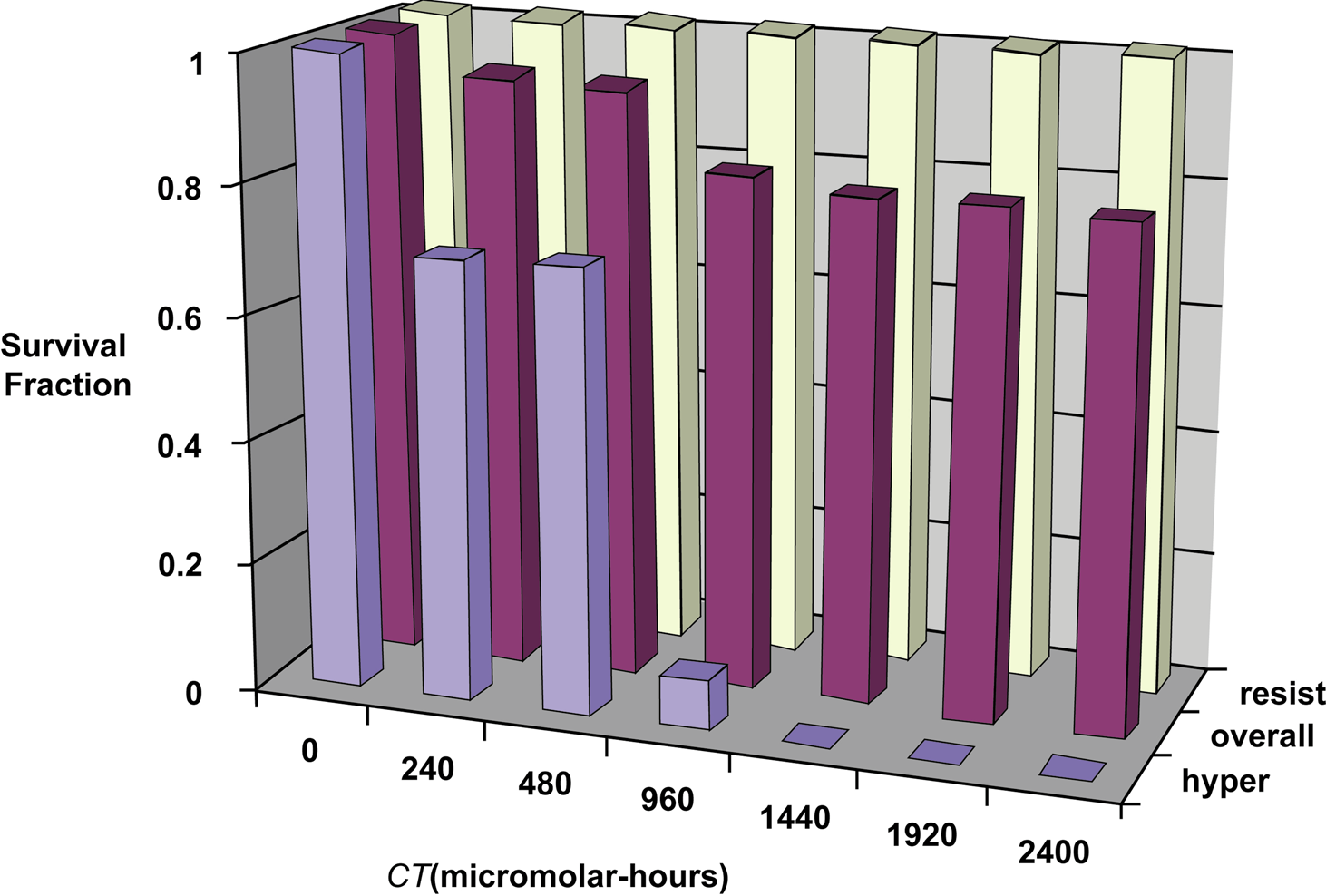
Results of exploratory analysis of SF data (averaged over replicate groups) of rat DRG somatosensory neurons reported by Prabhu et al. (2009) for in vitro exposure to 70.6 (± 20) -nm copper nanoparticles: overall–data as reported by Prabhu et al. (2009); resist–inferred resistant subfraction (data normalized for assumed 80% of population); hyper–inferred hypersensitive subfraction (data normalized to assumed 20% of population).

The data for hypersensitive cells in Figure 1 can be further analyzed to provide inferences on the underlying average hits (nanoparticle uptake) to the critical biological targets (presumed to be mitochondria) for lethality. Taking the natural logarithm of the average SF for the hypersensitive cells and multiplying the results by −1 gives the hypersensitive cell lethality hazard function, H _m(t) (Scott 2010); however, H _m(t) only can be evaluated in this way using dose groups for which not all cells are killed. The lethality hazard, H _m(t), then can be plotted vs. different dose metrics (CT, [CT]², [CT]³, etc.) to infer about the number of hits (on average) to the critical biological target (mitochondria) for lethality. The metric yielding an approximate straight line dose-response relationship then would be inferred as a useful dose metric for the indicated dose-response data and the power to which CT is raised would be an estimate of the on-average number of hits (nanoparticle uptakes by the mitochondria) for lethality. Subtracting 1 from this number then would yield an estimate mu of μ _m when mitochondria are the critical target. This approach has been used to obtain results presented in this paper.

With the estimate mu (= 1 or 2 or 3 etc.) obtained, it then can be used in the cumulative Poisson probability function P(round{mu}|E{M _m(t)}) to estimate the value of E{M _m(t)}* that yields a given value of E{SF}. The notation round{mu} means to round to the nearest integer. The ratio E{M _m(t)}*/CT is an estimate of the average of DCF _m, i.e., E{DCF _m}. Initial estimates of E{DCF _m}, μ_m , and E{f} then can provide guidance for constructing parameter prior distributions for use in Bayesian analysis to employ the STM model to data.

Figure 2 shows the best results obtained for plotting H _m(t) vs. [CT]ⁿ (for n = 1 or 2 or 3, etc.) and were obtained for n = 2 (implicating mu = 1 for an estimate of μ _m). The cumulative probability function P(1|E{M _m(t)}*) then was used to estimate E{M _m(t)}* for the data in Figure 1 for which CT = 960 molar-hours (lowest nonzero survival fraction level), by setting the function equal to the average, E{SF} =0.081, for the inferred hypersensitive sub-fraction and finding the value of E{M _m(t)}* that yielded the desired average SF value. Calculations were carried out using the Excel Goal Seek algorithm and corresponding Excel cumulative probability function POISSON(1, E{M _m(t)*}, true). This led to an estimate of E{DCF _m} of 0.0043 copper nanoparticle hits (particle uptakes) to mitochondria per micromolar-hour of exposure to copper nanoparticles.

FIGURE 2.

Lethality hazard for the inferred hypersensitive subfraction of DRG somatosensory neurons exposed in cell culture to 70.6 (± 20)-nm copper nanoparticles, based on data in Figure 1. The line was fitted to the highest dose point to see if the low-dose part of the line adequately represented the low-dose data when [CT]² (in micromolar²-hours²) is used as independent variable.

Modification of Equation 2 to Allow for Mixed Cell Population

To allow for a mixed population of neurons with a hypersensitive fraction f[1] = f and resistant fraction f[2] = 1 – f, which are assumed to vary over replicate groups, Equation 1 was modified so that the following applies:

$SF=f•\hspace{0.17em}\text{P}\left({\mu }_{\text{m}}|M_{\text{m}}\left(t\right)\right)+\left(1-f\right).$

(3)

When averaged over a large number of replicate groups, one gets the following which corresponds to Equation 2.

$E\{\hspace{0.17em}SF\}=E\left\{f\right\}•\hspace{0.17em}\text{P}\left({\mu }_{\text{m}}|E\{\hspace{0.17em}{M}_{\text{m}}\left(t\right)\}\right)+\left(1-E\left\{f\right\}\right).$

(4)

With the constructs for Equations 3 and 4, none of the resistant cells are killed. Only the hypersensitive sub-fraction fis presumed to be killed. Note that setting f = 1 in Equation 3 and E{f} = 1 in Equation 4 leads to Equations 1 and 2 which apply to a homogenous population. When employing Equation 4, μ _m should be rounded to the nearest integer. For example, μ _m = 0.05 should be rounded to 0. Similarly, μ _m = 1.05 should be rounded to 1.

Assignments of Prior Distributions for Model Parameters

Based on the above preliminary estimates for E{f}, μ _m, and DCF_m , and given the uncertainty associated with this modeling, rather broad prior distributions were assigned to the indicated parameters for the application of Bayesian analyses to fit Equation 4 to the data in Figure 1 for overall survival (averaged over replicate groups) of DRG somatosensory neurons exposed in vitro to 70.6 (± 20)-nm copper nanoparticles. The prior distribution assigned to E{f} was a uniform distribution with min = 0.0001 and max = 1 (brackets the preliminary estimate of 0.2). The prior distribution assigned to μ _m was uniform with min = 0 and max = 20 (brackets preliminary estimate mu = 1). The prior distribution assigned for the DCF _m was uniform with min = 0.001 and max = 0.01 (brackets the preliminary estimate 0.0043).

Because of concern for a linear relationship between M _m(t) and CT not applying for high levels of exposure, only data for the lowest four exposure levels (CT= 240, 480, 960, and 1440 micromolar-hours) were used initially in fitting the STM model to the cytotoxicity data. Table 1 shows the dosimetric results obtained with employing WinBUGS (Lunn et al. 2000) software to implement the STM model based on the data in Figure 1 for overall survival. The number of killed cells among 1500 neurons at risk per group (Prabhu et al. 2009) was assumed to have a binomial distribution with expectation value 1500(1-E{SF}) and variance 1500(1-E{SF})E{SF}. Plating efficiency is not addressed here and this may contribute some systematic error to estimates obtained for model parameters. Also because it was easier to obtain the posterior distribution for “μ _m + 1” (average hits to mitochondria required for lethality) with the approach used to fit the STM model to data, this is the statistic that is reported in Table 1.

TABLE 1.

Predicted dosimetric variable values based on the STM model and cell killing data of Prabhu et al. (2009) for in vitro application of 70.6 (± 20)-nm copper nanoparticles to somatosensory DRG neurons of the rat ¹

			Percentile
Endpoint	Posterior Distribution Mean	Standard Deviation	2.5%	50%	97.5%
E{DCF m} b	0.0032	2.7E-4	0.0027	0.0032	0.0037
μ m + 1	2	1.4	0.23	1.68	5.6
E{M m(t)} for CT = 240 c	0.76	0.065	0.64	0.76	0.89
E{M m(t)} for CT = 480 c	1.52	0.13	1.28	1.52	1.79
E{M m(t)} for CT = 960 c	3.05	0.26	2.57	3.04	3.57
E{M m(t)} for CT = 1440 c	4.57	0.39	3.85	4.56	5.36
E{M m(t)} for CT = 1920 c	6.1	-	-	-	-
E{M m(t)} for CT = 2400 c	7.62	-	-	-	-

a

Based on Bayesian inference implemented with MCMC using 15,000 iterations (10,000 burn-in) for lowest four dose groups.

b

Nanoparticle hits (uptake) to mitochondria per unit CT (i.e., micromolar-hours).

c

CT is the copper nanoparticle concentration time product in micromolar-hours.

In addition to μ _m + 1, endpoints listed in Table 1 are E{DCF _m} and E{M _m(t)} for the different levels of CT in Figure 1. For the MCMC analysis, the zero-dose group (controls) was excluded in order to avoid traps (stoppage of the program) in the computer code application. Total MCMC iterations were 15,000 with the first 10,000 results discarded as burn-in (uninformative data). Autocorrelation results obtained after the first 5,000 iterations suggested that a single long MCMC chain of 10,000 iterations should be sufficient for convergence. Thus, the 15,000 total iterations (10,000 burn-in + remaining 5000) used were presumed to be adequate for the investigations carried out.

The results in Table 1 for the highest two dose levels (1920 and 2400 micromolar-hours) were obtained with a separate MCMC analysis with E{DCF _m} fixed at the posterior mean (0.0032) obtained using only data for the lower 4 levels. All of the endpoints in Table 1, except μ _m + 1 had roughly Gaussian posterior distributions, suggesting that the reported standard deviations for the indicated distributions may be informative. However, the posterior distribution for μ _m + 1 had a mode of about 1–2 and a long tail to the right (departure from Gaussian). The posterior distribution mean and standard deviation for μ _m + 1 was 2 ± 1.4. The corresponding mean and standard deviation for μ _m is therefore 1 ± 0.4; essentially the same result as the initial estimate of μ _m = 1 based on Figure 2. When all of the six exposure groups were included in the analysis, an apparently biased estimate μ _m = 2 was obtained as the posterior distribution mean. The apparent bias is considered to relate to departure from a Poisson distribution for B _m(t) at high levels of exposure.

The results obtained imply that on average > 1 hit to each mitochondrion at risk is expected to be associated with significant cell killing via autophagy. For a point of reference, when M _m(t) = 2, then 86% of the mitochondria population among all target cells would be expected to have taken up at least 1 copper nanoparticle. Such a large number of hit mitochondria (those with particle uptake) for an individual cell might be expected to be sufficient to trigger a severe stress response. Thus, if mitochondria are indeed the critical target, multiple mitochondria may need to participate in the signaling that leads to the autophagic mode of death.

TABLE 2.

Posterior distribution statistics for the average survival fraction for overall survival and for the hypersensitive subfraction of somatosensory DRG neurons of the rat exposed in vitro to 70.6 (± 20)-nm carbon nanoparticles for 24 h based on the STM model and data of Prabhu et al. (2009). ^a

			Percentile
Endpoint	Posterior Distribution Mean	Standard Deviation	2.5%	50%	97.5%
E{f}	0.215	0.013	0.192	0.214	0.244
Hyper1 b	0.822	0.023	0.775	0.823	0.864
Hyper2 b	0.551	0.043	0.467	0.551	0.663
Hyper3 b	0.195	0.038	0.129	0.194	0.274
Hyper4 b	0.06	0.019	0.03	0.058	0.103
Hyper5 b	0.021	0.025	0.0021	0.015	0.056
Hyper6 b	0.006	0.009	4.6E-4	0.004	0.017
Overall1 c	0.962 (0.939) d	0.003	0.995	0.962	0.968
Overall2 c	0.904 (0.94) d	0.0054	0.893	0.904	0.914
Overall3 c	0.827(0.816) d	0.0057	0.816	0.827	0.838
Overall4 c	0.798 (0.796) d	0.009	0.78	0.798	0.815
Overall5 c	0.787 (0.783) d	0.0076	0.773	0.787	0.802
Overall6 c	0.784 (0.789) d	0.0077	0.769	0.784	0.799

a

Results for lowest four dose groups are based on Bayesian inference implemented with MCMC using 15,000 iterations (10,000 bur-in). Results for the highest two dose groups are based on 10,000 iterations (5,000 burn-in).

b

Hypersensitive cell survival statistics for groups Hyper1, Hyper2, … for the six nonzero dose groups starting from the lowest to the highest.

c

Overall cell survival statistics for groups Overall1, Overall2, … for the six nonzero dose groups starting from the lowest to the highest.

d

Experimentally observed average SF, based on reported average proportion of viable cells (Prabhu et al. 2009)

Table 2 gives the MCMC generated posterior distribution related statistics obtained for the average overall SF (overal1, overall2, …) and the average SF for the presumed hypersensitive sub-fraction (hyper1, hyper2, …) for the corresponding six levels of the CT product considered (level 1, CT = 240 micromolar-hours; level 2, CT = 480 micromolar-hours; level 3, CT = 960 micromolar-hours; level 4, CT = 1440 micromolar-hours; level 5, CT = 1920 micromolar-hours; level 6, CT = 2400 micromolar-hours). The average SFfor the presumed resistant sub-fraction was fixed at 1 and therefore no information related to this sub-fraction is provided in the table.

Roughly Gaussian posterior distributions were obtained for E{M _m(t)} for the four lowest exposure levels. The posterior distribution for the average fraction (E{f}) for the hypersensitive cells was also roughly Gaussian, with a mean of 0.215 and standard deviation of 0.013. The correlation between E{f} and μ _m was −0.02. The correlation between E{f} and E{DCF _m} was – 0.78. The correlation between E{DCF _m} and μ _m was 0.29. Thus, when employing the STM model using standard Monte Carlo, the indicated correlations need to be accounted for. Alternatively, one can rerun WinBUGS exactly as previously used to fit the STM model to the dose-response data, but this time also making predictions for endpoint of interest (e.g., E{SF} for new values of CT). This way the correlations will be automatically accounted for.

FIGURE 3.

Fitted cell population SF (middle curve; averaged over replicate groups) for DRG somatosensory neurons exposed in culture for t = 24-h to copper nanoparticles based on data from Prabhu et al. (2009) and the STM model. The independent variable is the posterior distribution mean for E{M _m(t)}. Data points are averages of experimental replicates (Prabhu et al. 2009). Also shown are predicted survival curves (population average) for the inferred resistant (upper horizontal line) and hypersensitive (bottom curve) neuron subfractions. All three curves apply only to 24hour exposure in virto.

Figure 3 gives STM-model-based average survival curves (based on Bayesian analysis posterior distribution means) for the overall mixed population and for the resistant and hypersensitive sub-fractions plotted as functions of E{M _m(t)}. The average SF values are based on Table 2 and calculated data points were simply connected using Excel's smoothing function. The experimental data of Prabhu et al. (2009) for the overall SF averaged over replicate groups are also shown in Figure 3. Thus, the smooth curves in Figure 3 are estimates of the population average SF. The statistics presented in Table 1 also apply to the population average SF.

Figure 4 shows the same curves as in Figure 3 but plotted vs. the corresponding values for the CT product in micromolar-hours. There is close agreement between the posterior distribution means for E{SF} in Figures 3 and 4 and the experimentally derived average SF data for the presumed mixed cell population. The maximum difference between the smooth curve for average overall survival and the data was < 0.05. Almost identical results (not shown) as presented in Table 2 for the average overall survival fraction (posterior distribution mean) was generated using the Equation 4 with parameters set at their posterior distribution means in Tables 1 and 2.

FIGURE 4.

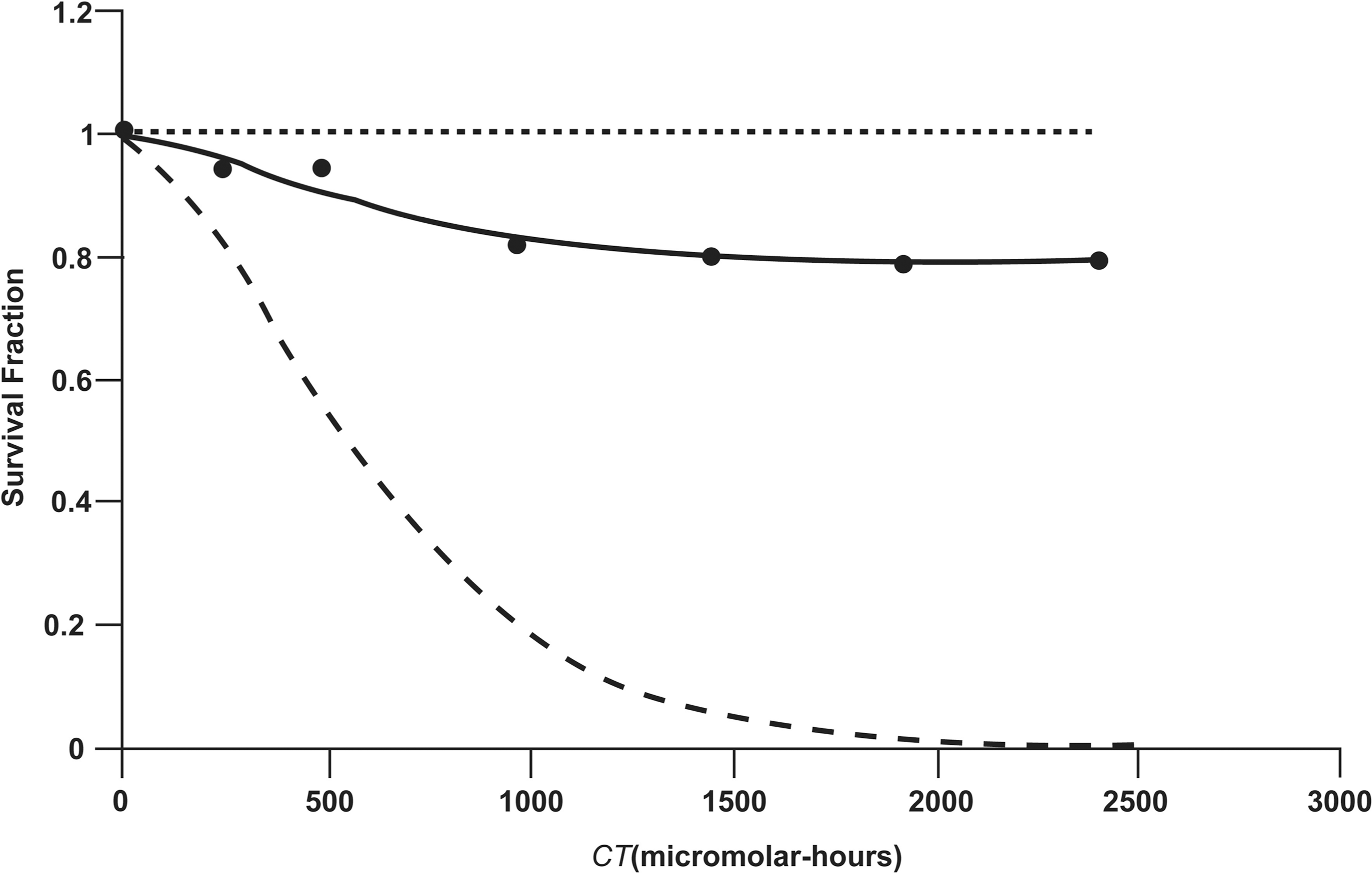
Same curves as in Figure 3 but plotted against CT (micromolar-hours).

DISCUSSION AND CONCLUSIONS

The estimate of 0.215 and standard deviation (0.013) for E{f} in Table 2 do not apply to individual replicate groups (especially the standard deviation); however, data for individual replicates can be analyzed as indicated below where individual SF data (43 data points) from replicate groups of Prabhu et al. (2009) are used. Two judged outliers were excluded. Forty-three different estimates of f were generated based on solving Equation 3 for f (which applies to a single replicate) with SF replaced by

$f*=\left(1-SF*\right)/[\hspace{0.17em}1-P\left(1|M_{\text{m}}\left(t\right)*\right)].$

(5)

Assuming that E{M _m(t)} has a relatively small coefficient of variation, an estimate E{M _m(t)}* based on averaging over replicate studies can be used as an initial estimate (to be refined) of M _m(t) in Equation 5. For data points for which SF* = 1, they were temporarily set to 0.99 when evaluating f* to ensure values > 0 (an assumption). This was especially important for the lowest exposure group for which CT = 240 micromolar-hours. The scatter in the value of f* for the different exposure groups were quite similar for all except for the lowest exposure group (CT=240 micromolar-hours) as demonstrated in Figure 5. Greater variability is associated with the exposure group for which CT=240 micromolar-hours, which relates in part to uncertainty in the observed SF data. The individual data for f* ranged from 0.03 to 0.62, suggesting considerable biological variability in the replicate cultures used by Prabhu et al. (2009). The values for f* were not correlated with CT (R ² = 0.0014, p > 0.5).

FIGURE 5.

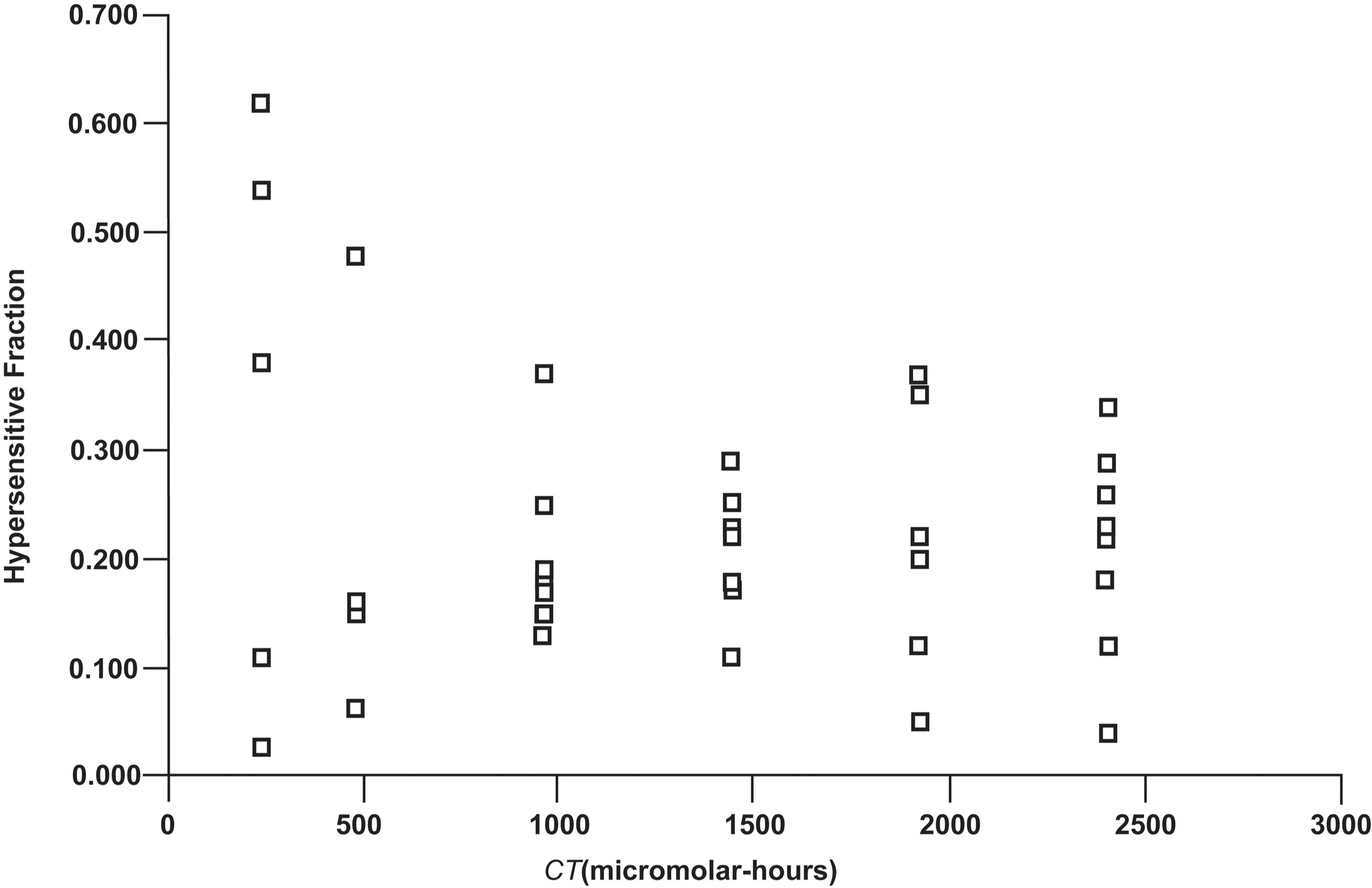
Variability in the estimates f* of f (fraction of hypersensitive DRG neurons) plotted vs. the different values for CT (micromolar-hours) used by Prabhu et al. (2009).

Averages of f* and the associated standard deviations by the exposure group were 0.25±0.26 (CT=240), 0.20 ± 0.16 (CT=480), 0.20 ± 0.08 (CT=960), 0.21 ± 0.06 (CT=1440), 0.21 ± 0.11 (CT=1920), and 0.21 ± 0.1 (CT=2400). Thus, these 6 averages (over replicates) are reasonably similar to the posterior distribution mean for E{f} reported in Table 2 which is based on fitting the STM model to data for the average SF for the replicates. The un-weighted mean of these 6 estimates and standard error are 0.214 ± 0.021, which are close to the results in Table 2 for the posterior distribution mean (i.e., 0.215 ± 0.0130). Note also that the standard deviations for each of the 6 estimates above are larger than the standard deviation in Table 2 for the posterior distribution of E{f}.

The indicated 43 values for f* were used in Equation 3 along with μ _m = 1 to find new (refined) values of M _m(t)* that yield the observed values for SF. Computations were carried out in Excel using the Goal Seek algorithm. One simply finds the value for M _m(t)* that makes Equation 3 corresponded to the desired value for SF*. This led to 43 new estimates for M _m(t)* which are plotted in Figure 6 (some overlapping). The data in Figure 6 are correlated with CT (R ² = 0.856, p < 0.001) and show clear saturation (i.e., nonlinear) at high levels of CT. The results obtained suggest that on average not more than about eight of the 70.6 (± 20)-nm copper nanoparticle can be taken up by mitochondria of DRG somatosensory neurons in cell culture. This needs to be verified experimentally.

FIGURE 6.

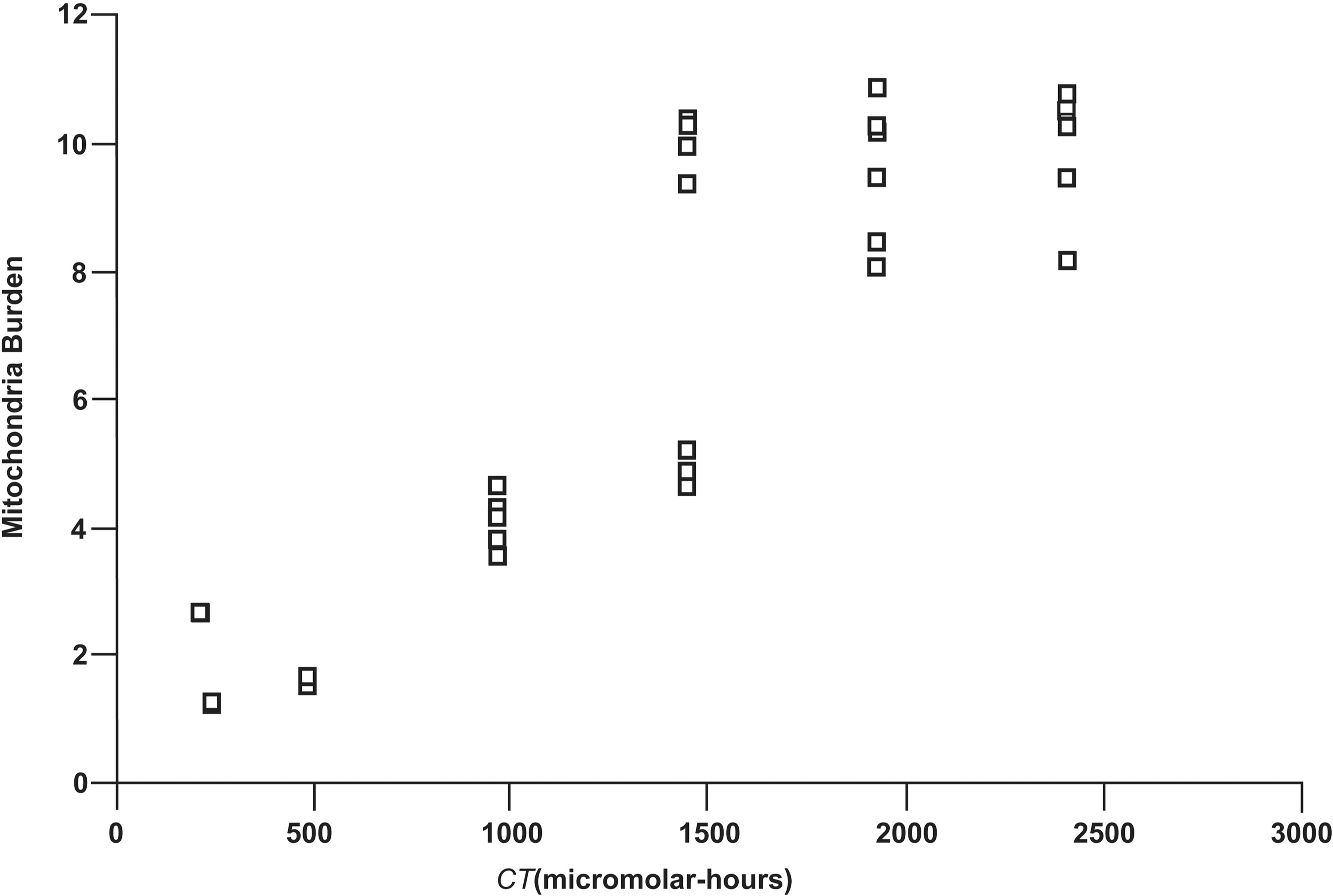
Variability in the estimates M _m(t)* of the mitochondria burden M _m(t) plotted vs. the different values for CT (micromolar-hours) used by Prabhu et al. (2009).

Unlike the pmf Φ _m(N _m) which is independent of M _m(t), the presumed Poisson distribution Ψ_t(B_m(t)) of B _m(t) changes as M _m(t) changes and can be displayed using the Excel function POISSON(n, M(t), false), with n taking on target hit numbers (nanoparticle uptakes) 0, 1, 2, etc. This is illustrated in Figure 7 where values are assigned to M _m(t) based on the exposure-group-specific posterior distribution means in Table 1. Similarly, the distribution (an estimate) of the threshold hits (nanoparticles uptakes), N _m, to be exceeded for lethality can be displayed using the Excel function POISSON (n, μ _m, false). This is illustrated in Figure 8 based on μ _m having a value of 1.

FIGURE 7.

Predicted Poisson distribution probability mass function Ψ_t(B _m(t)) for the specific mitochondrion burden, B _m(t), for the following predicted values of the mitochondria burdens M _m(t) based on results in Table 1: Mm1, M _m(t) = 0.76; Mm2, M _m(t) = 1.52; Mm3, M _m(t) = 3.05; Mm4, M _m(t) = 4.57; Mm5, M _m(t) = 6.1; Mm6, M _m(t) = 7.62.

FIGURE 8.

Predicted Poisson distribution probability mass function Φ_m(N _m) of the number N _m of mitochondrion hits (nanoparticle uptake) by copper nanoparticles to be exceeded (stochastic threshold) for triggering presumed autophagic-mode death in hypersensitive DRG neurons in culture when μ _m = 1 as implicated for the posterior distribution mean of μ _m + 1 in Table 1.

The variability in the SF values over replicate groups due to variability in M _m(t) and in f can be addressed in the context of the STM model as illustrated in Figure 9. The central curve was generated using Equation 3 with parameter value assignments of μ _m = 1 and f = 0.215. The upper jagged curve (data points joined by straight lines) is based on the calculated maximum values for SF and the lower curve is based on calculated minimum values using the different exposure-group specific values for f* and M _m(t)* in Figures 5 and 6. The parameter μ _m was fixed at 1, which is presumed to be a reliable estimate. Thus, the variability was ascribed to variability in f and M _m(t). It follows that the STM model (as applied here) not only adequately represents the dose-response curve for the average survival (Figures 3 and 4) but also provides a plausible explanation of the variability in SF data over replicate groups (Figure 9). The explanation is that different values for f and M_m (t) apply to different replicate groups.

Variability in f is biological variability likely related to the cell culture sample selection process. Variability in M _m(t) likely relates to variability in the copper nanoparticle particokinetics and may also relate to variability in CT for a given intended exposure level (e.g., CT = 240 micromolar-hours intended but CT = 250 micromolar-hours actually achieved for a given replicate group).

FIGURE 9.

Variability over replicate groups in the SF data of Prabhu et al. (2009) for 70.6 (± 20)-nm copper nanoparticle induced cytoxicity to DRG neurons in culture. The central, upper and lower curves are based on the STM model as explained in the main text.

Modeling results obtained indicate that when the average of the specific mitochondrion burden (organelle hits) of nanoparticles exceeds 1 particle per each mitochondrion, significant killing of the inferred hypersensitive subpopulation is expected to occur. When M _m(t) = 2, then 86% of the mitochondria would be expected to contain at least one nanoparticle. Thus, multiple mitochondria in a given target cell may be involved in signaling for triggering the presumed autophagic mode of cell death. Further, the results obtained suggest that there appears to be an upper limit to the number of copper nanoparticles that can be taken up (possibly < 10) by a given mitochondrion.

If there is a limit on the number of nanoparticles that can be taken up by a given mitochondrion (e.g., < 10), then the distribution cannot be Poisson when the mean burden is close to 10. Thus, the distributions presented in Figure 7 may be in error for M _m(t) >> 1. This could be addressed by truncating the Poisson distribution and reassigning probability mass for specific burdens > than a maximum burden B _m,max into the probability mass Ψ_t(B _m,max); however, this issue will have to be addressed in future research.

The number of hypersensitive DRG somatosensory neurons destroyed by copper nanoparticles is predicted to increase as the mitochondria burden (average of specific mitochondrion burdens) of nanoparticles increases, as could occur after repeated skin applications of material containing the particles. Further, the results presented suggest that repeated low-level exposure (e.g., over years) of humans to copper nanoparticles could eventually lead to complete destruction of the implicated hypersensitive subpopulation of neurons. Thus, it is important for researchers to focus on identifying these cells (if they exist) and identify their functions. In addition, surviving hypersensitive and resistant cells may have dysfunctional mitochondria after moderate and high level exposure to copper nanoparticles which could lead to nervous system dysfunction and related morbidity.

In circumstances where more than two sub-fractions of cells of varying sensitivity (with sensitivity evaluated as 1/μ_m) are involved and there is a single mode of death (autophagic), one can evaluate the contribution to the overall survival for the j ^th sub-fraction using f[j]•P(μ _m[j]| M _m[j]), where the parameters f[j] and μ _m[j], and variable M _m[j] correspond to f, μ _m, and M _m(t) for a homogenous population of cells. The different sub-fractions f[j] must however sum to 1 as was the case used here where f[1] = f (hypersensitive cells) and f[2] = 1 – f (resistant cells).

The relative sensitivity (RS) of a subfraction j relative to a subfraction k can be evaluated as follows:

$RS[\hspace{0.17em}j,k]=\left(1/{\mu }_{\text{m}}\left[j\right]\right)/\left(1/{\mu }_{\text{m}}\left[k\right]\right)={\mu }_{\text{m}}\left[k\right]/{\mu }_{\text{m}}\left[j\right].$

(6)

Even though the critical target modeled here was assumed to be mitochondria, a similar approach would apply if the critical target was the entire cell, cytoplasm, nucleus or another organelle in the cell that takes up nanoparticles. For multiple modes of cell killing (e.g., damage to mitochondria, damage the nucleus, damage to membranes, etc.), an approach similar to the approach described elsewhere (Scott 2010) can be used.

The STM model cannot by itself be applied for in vivo exposure of the skin to MENAP because exposure of the skin does not necessarily mean that the particles will reach a target cell population of interest. For in vivo toxicity assessment, the model has to be coupled with particokinetics (systemic and other transport) and particodynamics (tissue, cell, and organelle uptake and retention) models. Also, copper nanoparticles tend to agglomerate (Prabhu et al. 2009) and this has not been addressed in the present application of the STM model. Even so, individual copper nanoparticles would be expected to be more efficiently taken up by neurons and their organelles than agglomerates; thus, the mathematical relationships presented would be expected to also apply to individual nanoparticles released from extracellular agglomerates that entered neurons as single nanoparticles. In addition, the mathematical relationships presented could also be applied to individual atoms released from extracellular nanoparticles via dissolution. In this case B _m(t) would represent the number of atoms (e.g., copper) contained in a given mitochondrion at exposure time t.

Different research groups sometimes evaluate nanoparticle concentrations using different approaches. Thus, what is reported as a nanoparticle concentration in micromolar units may vary between different research groups when applying the same amount of material to the same volume. This will impact on the value derived for DCF _m but not on the microdosimetric spectra generated for B _m(t) using the STM model. This is because microdosimetric spectra are derived via biological micro-dosimetry that relates to the observed cell survival fractions.

The title of this paper poses the rather important question: “Are some neurons hypersensitive to metallic nanoparticles?” While the question has not been convincingly answered, sufficient indirect evidence is presented implicating the existence of hypersensitive neurons; thus, there is a need for more experimental research that directly addresses the question. An additional question should also now be posed that also relates to new research needs: Are neurons that survive MENAP hits to the majority of mitochondria dysfunctional and if so can the dysfunction contribute to neurological diseases?

While the results presented relate to concerns about skin application of MENAP, other routes of exposure (e.g., inhalation, ingestion) could also lead to nervous system damage as well as to damage to other body organs (e.g., lung, heart, liver, etc.). Further, cells in these other organs that survive MENAP damage could be dysfunctional and thereby contribute to organ dysfunction and related morbidity. Thus, it is important that regulatory agencies, nanotechnology organizations, and the general public be aware of these possibilities and institute protective measures as necessary.